Attributing the 2017 Bangladesh floods from meteorological and hydrological perspectives - HESS
←
→
Page content transcription
If your browser does not render page correctly, please read the page content below
Hydrol. Earth Syst. Sci., 23, 1409–1429, 2019
https://doi.org/10.5194/hess-23-1409-2019
© Author(s) 2019. This work is distributed under
the Creative Commons Attribution 4.0 License.

Attributing the 2017 Bangladesh floods from meteorological and
hydrological perspectives
Sjoukje Philip1 , Sarah Sparrow2 , Sarah F. Kew1 , Karin van der Wiel1 , Niko Wanders3,4 , Roop Singh5 ,
Ahmadul Hassan5 , Khaled Mohammed2 , Hammad Javid2,6 , Karsten Haustein6 , Friederike E. L. Otto6 ,
Feyera Hirpa7 , Ruksana H. Rimi6 , A. K. M. Saiful Islam8 , David C. H. Wallom2 , and Geert Jan van Oldenborgh1
1 Royal  Netherlands Meteorological Institute (KNMI), De Bilt, the Netherlands
2 Oxford   e-Research Centre, Department of Engineering Science, University of Oxford, Oxford, UK
3 Department of Physical Geography, Utrecht University, Utrecht, the Netherlands
4 Department of Civil and Environmental Engineering, Princeton University, Princeton, NJ, USA
5 Red Cross Red Crescent Climate Centre, The Hague, the Netherlands
6 Environmental Change Institute, Oxford University Centre for the Environment, Oxford, UK
7 School of Geography and the Environment, University of Oxford, Oxford, UK
8 Institute of Water and Flood Management, Bangladesh University of Engineering and Technology, Dhaka, Bangladesh

Correspondence: Sjoukje Philip (sjoukje.knmi@gmail.com) and Geert Jan van Oldenborgh (oldenbor@knmi.nl)

Received: 10 July 2018 – Discussion started: 23 July 2018
Revised: 14 February 2019 – Accepted: 14 February 2019 – Published: 13 March 2019

Abstract. In August 2017 Bangladesh faced one of its worst           change in discharge towards higher values is somewhat less
river flooding events in recent history. This paper presents,        uncertain than in precipitation, but the 95 % confidence inter-
for the first time, an attribution of this precipitation-induced     vals still encompass no change in risk. Extending the analy-
flooding to anthropogenic climate change from a combined             sis to the future, all models project an increase in probability
meteorological and hydrological perspective. Experiments             of extreme events at 2 ◦ C global heating since pre-industrial
were conducted with three observational datasets and two             times, becoming more than 1.7 times more likely for high 10-
climate models to estimate changes in the extreme 10-day             day precipitation and being more likely by a factor of about
precipitation event frequency over the Brahmaputra basin up          1.5 for discharge. Our best estimate on the trend in flooding
to the present and, additionally, an outlook to 2 ◦ C warming        events similar to the Brahmaputra event of August 2017 is
since pre-industrial times. The precipitation fields were then       derived by synthesizing the observational and model results:
used as meteorological input for four different hydrological         we find the change in risk to be greater than 1 and of a similar
models to estimate the corresponding changes in river dis-           order of magnitude (between 1 and 2) for both the meteoro-
charge, allowing for comparison between approaches and for           logical and hydrological approach. This study shows that, for
the robustness of the attribution results to be assessed.            precipitation-induced flooding events, investigating changes
   In all three observational precipitation datasets the climate     in precipitation is useful, either as an alternative when hydro-
change trends for extreme precipitation similar to that ob-          logical models are not available or as an additional measure
served in August 2017 are not significant, however in two out        to confirm qualitative conclusions. Besides this, it highlights
of three series, the sign of this insignificant trend is positive.   the importance of using multiple models in attribution stud-
One climate model ensemble shows a significant positive in-          ies, particularly where the climate change signal is not strong
fluence of anthropogenic climate change, whereas the other           relative to natural variability or is confounded by other fac-
large ensemble model simulates a cancellation between the            tors such as aerosols.
increase due to greenhouse gases (GHGs) and a decrease due
to sulfate aerosols. Considering discharge rather than precip-
itation, the hydrological models show that attribution of the

Published by Copernicus Publications on behalf of the European Geosciences Union.
1410 S. Philip et al.: Attributing the 2017 Bangladesh floods
1 Introduction 30 years to an event occurring once in 100 years, depend-
ing on the data source: water level and discharge data at
In August 2017 Bangladesh faced one of the worst river Bahadurabad (the main station for discharge representing
flooding events in recent history, with record high water lev- the Brahmaputra in Bangladesh) and the flooding forecast
els, and the Ministry of Disaster Management and Relief re- system GloFAS. These estimates, however, were implicitly
ported that the floods were the worst in at least 40 years. based on the assumption of a stationary climate and did not
Due to heavy local rainfall, as well as water flow from account for the possibility that the frequency of such flooding
the upstream hills in India, the various rivers in northern events may be changing.
Bangladesh burst their banks. This led to the inundation of Extreme rainfall events that subsequently lead to
river basin areas in the northern parts of Bangladesh, starting widespread flooding, such as the 2017 event in Bangladesh,
on 12 August and affecting over 30 districts. The National are one of the main types of extreme weather events that we
Disaster Response Coordination Centre (NDRCC) reported are expecting to see more of in a warming climate. But with
that around 6.9 million people were affected, with 114 peo- rainfall not only being driven by thermodynamic processes
ple reported dead and at least 297 250 people displaced. Ap- but also being affected by changing atmospheric processes,
proximately 593 250 houses were destroyed, leaving families it is not clear a priori if such events at a particular location
displaced in temporary shelters. will increase in likelihood or if the dynamic changes will
Bangladesh is a highly flood-prone country, with flat to- mean that the overall chance of extreme rainfall decreases
pography and many rivers that regularly flood and are used to there (Otto et al., 2016). Furthermore, in the current climate,
irrigate crops and for fishing. The August 2017 floods were drivers other than greenhouse gases (GHGs) often play a
particularly impactful as they followed two earlier flooding role that is currently difficult to quantify but likely to mask
episodes in late March and July that year, increasing the vul- or exacerbate the effect of greenhouse-gas emissions so far
nerability of people. Nearly 85 % of the rural population in on the occurrence likelihood of extreme rainfall events (e.g.
Bangladesh works directly or indirectly with agriculture, and aerosols, van Oldenborgh et al., 2016). Hence regional attri-
rice is the main staple food, contributing to 95 % of total bution studies are necessary for identifying whether and to
food production. As is typical after such flooding, farmers what extent extreme rainfall events are changing and for pro-
started to plant aman, the monsoon rice that is almost en- viding insight into which drivers have been contributing to
tirely rain dependent. However, the August flood was worse those changes and whether the trend is likely to continue into
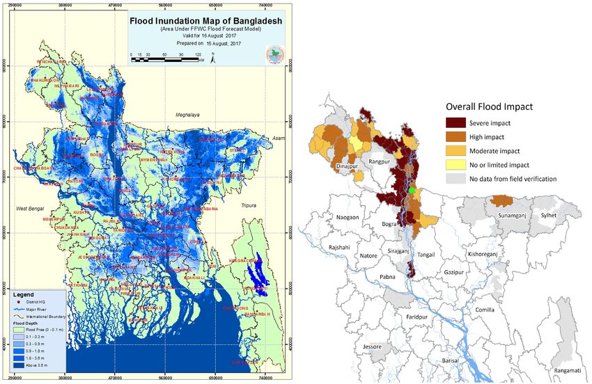
than that of July, and areas such as Dinajpur and Rangpur that the future. Attribution studies require both observational data
normally do not flood were also flooded (see Fig. 1). These and models to fully estimate the impact of changes in the cli-
are areas that contain significant rice production. As a result, mate system. The reported advances in model development
650 000 ha of croplands were severely damaged during the for the Brahmaputra region and their success in forecasting
August monsoon flooding in the year. Aman rice is histori- gives good confidence in the models’ ability to accurately
cally the most variable, and yields tend to drop dramatically represent the region.
during major flood years (Yu et al., 2010). The flood-induced Hydrological models are increasingly used for studies on
crop losses in 2017 resulted in the record price of rice, nega- flooding in Bangladesh. As upstream flow data are absent for
tively affecting livelihood and food security. Beyond impacts Bangladesh, a lot of effort has been made to develop flood
to agriculture, the floods destroyed transport infrastructure forecasting systems based on satellite data and weather pre-
such as railways lines, bridges and roads, leaving some areas dictions. Webster et al. (2010), for instance, developed a sys-
inaccessible to disaster relief efforts. The rise in water and tem that forecasts the Ganges and Brahmaputra discharge
strong current breached roads and embankments and swept into Bangladesh in real time on 1-day to 10-day time hori-
away livestock, houses and assets that may have otherwise zons. In a recent study Priya et al. (2017) show that, by using
been protected. At least 2292 schools were damaged, affect- a new long lead flood forecasting scheme for the Ganges–
ing education for weeks, and 13 035 cases of waterborne ill- Brahmaputra–Meghna basin, skillful forecasts are provided
nesses were reported in the aftermath of the floods. that inherently not only express a prediction of future water
The 2017 flood was markedly different from previous ma- levels but also supply information on the levels of confidence
jor flood events in 1988 and 1998, when both the Ganges and with each forecast. Hirpa et al. (2016) used reforecasts to im-
Brahmaputra flooded simultaneously (Webster et al., 2010). prove the flood detection skill of forecasts.
Based on forecasts it was feared that a similar event would Previous scientific studies generally show an increasing
occur in 2017, but in this case, the swelling of the Brahmapu- trend in climate projections of extreme rainfall and high dis-
tra; its tributary, the Atrai; and the Meghna caused flooding. charge in the region. For example, Gain et al. (2011) use the
The worst impacts were along the main reach of the Brahma- PCR-GLOBWB model with input from 12 global circula-
putra River (Fig. 1b). tion models (GCMs; 1961–2100) from the CMIP3 ensemble
The first estimates of the return period provided by the (Meehl et al., 2007) in a weighted ensemble analysis. They
Bangladesh Water Development Board (BWDB) for the show that in this ensemble, there is a positive trend in the
2017 flood event range from an event occurring once in peak flow at Bahadurabad; in this model configuration and
Hydrol. Earth Syst. Sci., 23, 1409–1429, 2019 www.hydrol-earth-syst-sci.net/23/1409/2019/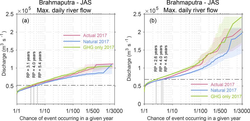
S. Philip et al.: Attributing the 2017 Bangladesh floods                                                                             1411

Figure 1. Inundation forecast map of Bangladesh for 16 August 2017 (left panel). Overall flood impact of the August 2017 flooding as
stated on 21 August (right panel). The green circle in the northwest of the map denotes the location of Bahadurabad. The Brahmaputra
basin is outlined in Fig. 3; see the original documents (source: Flood Forecast and Warning Center – FFWC – of BWDB at https://reliefweb.
int/sites/reliefweb.int/files/resources/SitRep_2_BangladeshFlood_16August2017.pdf, last access: 8 May 2018 and https://reliefweb.int/sites/
reliefweb.int/files/resources/72hrs-Bangladesh_Flood_Version1_Final08212017.pdf, last access: 8 May 2018) for more details on the maps
and legends.

under the SRES B2 scenario, a peak flow that currently oc-              semble. Zaman et al. (2017) use two sets of climate models
curs every 10 years will occur at least once every 2 years              with climate change runs under the RCP8.5 scenario as in-
during the time period 2080–2099. Dastagir (2015) gives an              put in a basin model that simulates flows in major rivers of
overview of the change in flooding according to the IPCC                Bangladesh, including the Brahmaputra. Using the two cli-
5th Assessment Report, using 16 GCMs from the CMIP5                     mate model runs as input, they find agreement in the basin
ensemble (Taylor et al., 2012). They state that the warmer              model runs for Brahmaputra flow in a 2.0 ◦ C warmer world;
and wetter climate predicted for the Ganges–Brahmaputra–                one run shows a slightly higher impact of climate change
Meghna basin by most climate-related research in this re-               compared to the other run, with an overall increase in mon-
gion indicates that vulnerability to severe monsoon floods              soon flow of approximately 15 % and 10 % in the dry season.
will increase with climate change in the flood-prone areas of              Attribution studies on flooding, using both observational
Bangladesh. The same conclusion is reached by CEGIS and                 data and models, have often been done with precipitation
SEN authors (2013), who use GCM projections and a hydro-                only. In such studies, (e.g. Schaller et al., 2014; van der Wiel
logical model to show that in the wet season, an increase in            et al., 2017; Philip et al., 2018; van Oldenborgh et al., 2017;
precipitation and annual flow is projected. In line with this,          Risser and Wehner, 2017) it is assumed that precipitation is
Mohammed et al. (2017) find that in a 2.0 ◦ C warmer world,             the main cause of the flooding. For shorter timescales and
floods will be both more frequent and of a greater magni-               the relatively small basins involved, this is a reasonable as-
tude than in a 1.5 ◦ C warmer world in Bangladesh, using                sumption. The major basins in Bangladesh, however, are sub-
the hydrological model the Soil and Water Assessment Tool               stantially larger and have longer water travel times than the
(SWAT) with input from the CORDEX regional model en-                    basins considered in the above studies. Therefore using pre-

www.hydrol-earth-syst-sci.net/23/1409/2019/                                           Hydrol. Earth Syst. Sci., 23, 1409–1429, 2019
1412                                                                   S. Philip et al.: Attributing the 2017 Bangladesh floods

cipitation alone as a proxy for flooding might not be appro-       cussion follows in Sect. 6, and the paper ends with some con-
priate. In this paper we explicitly test this assumption by per-   clusions.
forming an attribution of both precipitation and discharge as
a flooding-related measure of climate change. Thus we ex-
plore the flood in two different ways – first from a meteoro-      2     Data and methods
logical perspective (using precipitation data) and then from
a hydrological perspective (using discharge data). Schaller        Observational data are described in Sect. 2.1, and the mod-
et al. (2016) already studied a flooding case in an attribution    els and experiments are described in Sect. 2.2. The explana-
study using one hydrological model. Yuan et al. (2018) use         tion of how these data are used in the analysis is detailed in
observations, GCMs, and one land surface model with and            Sect. 2.3.
without land cover change to split the changes in observed
                                                                   2.1    Observational data
streamflow and its extremes into anthropogenic and natural
climate change, land cover change and human-water with-            The first observational dataset we use is the 0.5◦ gauge-based
drawal components. In this paper we do an attribution study        CPC analysis from 1979 to now (https://www.cpc.ncep.
for the first time using observational precipitation and dis-      noaa.gov/products/Global_Monsoons/gl_obs.shtml, last ac-
charge data and a combination of GCMs and several hydro-           cess: 20 March 2018). This is the longest gauge-based daily
logical models. To compare the differences between the at-         gridded dataset available that is still being updated. The
tribution results for the two variables we calculate the return    seasonal cycle of precipitation in the Brahmaputra basin is
periods and risk ratios for the August 2017 flooding event in      shown in Fig. 2a. Monsoon rains start rising slowly, with a
Bangladesh for both precipitation and discharge in observa-        maximum in July and August, and become less from Septem-
tions and models, for past (pre-industrial), present and future    ber onwards. As precipitation will not, in general, cause
(2◦ warmer than pre-industrial) conditions.                        flooding before July, we will use the months JAS for the pre-
    Bangladesh is influenced by three large river basins: the      cipitation analysis.
Ganges basin in the northwest, the Brahmaputra basin in the           The second gauge-based dataset we use for comparison is
northeast and the Meghna basin in the east. During the mon-        the combined Full Data and First Guess Daily 1.0◦ GPCC
soon season the rainfall moves northwest across the coun-          dataset (1988–now) (Schamm et al., 2013, 2015). As this is
try, starting in May–June–July in the Meghna basin. Usu-           a much shorter dataset we expect the signal-to-noise ratio in
ally 2–3 weeks after peak rainfall in July, the rivers in the      the trend to be smaller. We only use this dataset to addition-
Brahmaputra basin reach their peak discharge. Finally, in Au-      ally check the observations. The seasonal cycle can be found
gust and September the Ganges basin river discharge peaks.         in the Supplement Fig. S1.
The largest impact of flooding in August 2017 was felt in             The third dataset is the reanalysis dataset ERA-interim
the northern parts of Bangladesh (Fig. 1). As this was mainly      (ERA-int; 1979–now; Dee et al., 2011). Precipitation of this
caused by precipitation in the Brahmaputra basin, the focus        dataset is analysed directly. As well as precipitation, tem-
in this paper will be on this basin. In the Brahmaputra basin      perature and potential evapotranspiration (calculated with the
little water originates from precipitation on the northern side    Penman–Monteith method) are used to drive one of the hy-
of the Himalaya (China–Tibet), with most of the water com-         drological models (see Sect. 2.2.2). The seasonal cycle of
ing from precipitation in the upstream Assam region in India.      ERA-int can be found in Fig. S1.
Precipitation in Bhutan also contributes to the river water in        We use discharge and water level data from Bahadurabad.
Bangladesh.                                                        Discharge data are available for the years 1984–2017, and
    In this paper we use two event definitions: one based on       water level data are available for the years 1985–2017
precipitation and one based on discharge. Both observational       (source: BWDB). For both datasets the seasonal cycle is
data and model data can be used for these two event defini-        shown in Fig. 2b, c. Additionally, we have a discharge dataset
tions. For precipitation we average over the whole Brahma-         for the years 1956–2006 (source: BWDB). As the rating be-
putra basin and take a 10-day average, as the largest precipi-     tween water level, velocity and discharge is not exactly the
tation volume in the Brahmaputra basin travels to Bangladesh       same in the two discharge datasets, we consider simply merg-
within 10 days; see Fig. 5 in Webster et al. (2010). Only pre-     ing the datasets not to be appropriate. The 1984–2017 dataset
cipitation in July–August–September (JAS) is analysed as it        is used in the analyses, but results are compared to calcula-
is only in these months that precipitation is considered the       tions with the 1956–2006 dataset and merged datasets.
major cause of flooding. For discharge we simply use the
daily maximum discharge at Bahadurabad, a station situated         2.2    Model descriptions
to the north of the confluence point of the Ganges with the
Brahmaputra, in JAS.                                               First the global circulation model and regional model that
    The data and methods used are described in Sect. 2. Sec-       are used for the analysis of precipitation are listed, including
tions 3 and 4 describe the analysis for observations and mod-      a short description of the model runs. Next a list of hydrolog-
els respectively. The results are synthesized in Sect. 5. A dis-   ical models used in this study is given. Further details of the

Hydrol. Earth Syst. Sci., 23, 1409–1429, 2019                                    www.hydrol-earth-syst-sci.net/23/1409/2019/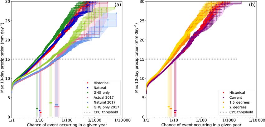
S. Philip et al.: Attributing the 2017 Bangladesh floods                                                                         1413

Figure 2. Seasonal cycle of (a) precipitation in the Brahmaputra basin for CPC, (b) discharge at Bahadurabad and (c) water level at Ba-
hadurabad. The red line shows the mean value, and green lines show the 2.5, 17, 83 and 97.5 percentiles.

models, including validation and calibration of the hydrolog-            See the Supplement for a more detailed description of
ical models, are described in the Supplement.                         these runs.

2.2.1   Precipitation                                                 2.2.2   Discharge

EC-Earth 2.3                                                          PCR-GLOBWB 2

We use three different ensembles of the coupled atmosphere–           The global hydrological model PCR-GLOBWB 2 (Sutanud-
ocean general circulation model EC-Earth 2.3 (Hazeleger               jaja et al., 2018) was selected because of its ability to
et al., 2012) at T159 (∼ 150 km). The first one is a transient        simulate the hydrological cycle, including reservoir opera-
model experiment, consisting of 16 ensemble members cov-              tions and human–water interactions at continental and global
ering 1861–2100 (here we use up to 2017), which are based             scales. It resolves the water balance at the surface by us-
on the historical CMIP5 protocol until 2005 and are based             ing precipitation, temperature and potential evaporation in-
on the RCP8.5 scenario (Taylor et al., 2012) from 2006 on-            puts from meteorological observations or climate models.
wards. The other two EC-Earth 2.3 experiments are two time-           We used PCR-GLOBWB to conduct several river discharge
slice experiments based on the 16-member transient model              simulations, First we used observational data as input to
experiment above. Two experimental periods are selected in            check the performance of the model. Next we used the EC-
which the model global mean surface temperature (GMST)                Earth transient and two time-slice experiments as input to
is as observed in 2011–2015 (“present-day” experiment) and            generate a large ensemble.
the pre-industrial (1851–1899) +2 ◦ C warming experiment
(“2 ◦ C warming” experiment).                                         SWAT

weather@home                                                          Second, we use the SWAT, which is a commonly used hy-
                                                                      drological model for investigating climate change impacts
In addition to the EC-Earth 2.3 experiments, large ensembles          on water resources at regional scales (Gassman et al., 2014).
of climate model simulations are created using the distributed        This model has already been used to simulate impacts of cli-
computing weather@home modelling framework (Guillod                   mate change on the flows of the Brahmaputra River (Mo-
et al., 2017; Massey et al., 2014) based on Hadley Cen-               hammed et al., 2017, 2018). The water balance equation used
tre models. Table 1 describes the experiments used in this            in SWAT consists of daily precipitation, runoff, evapotran-
study, which are grouped into three sets: (i) ensembles for           spiration, percolation and return flow. The SWAT model was
the historical period 1986–2015, (ii) ensembles for 2017 and          used in this study to simulate flows by taking inputs from
(iii) ensembles for assessing possible changes in the future.         both the transient and time-slice EC-Earth experiments and

www.hydrol-earth-syst-sci.net/23/1409/2019/                                        Hydrol. Earth Syst. Sci., 23, 1409–1429, 2019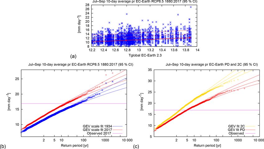
1414                                                                     S. Philip et al.: Attributing the 2017 Bangladesh floods

Table 1. Experiments with the weather@home ensemble.

      Category        Experiment       Description
      Climatology     Historical       1986–2015 SSTs and sea ice as observed, other forcings from CMIP5 historical+RCP4.5
                      Natural          1986–2015, SSTs reconstructed for pre-industrial conditions, all other forcings pre-industrial
                      GHG only         1986–2015, SSTs reconstructed for GHG emissions only, CMIP5 historical+RCP4.5 GHG
                                       emissions, all other forcings pre-industrial
      2017 specific   Actual 2017      2017 SSTs and sea ice as observed, other forcings as RCP4.5
                      Natural 2017     2017, SSTs reconstructed for pre-industrial conditions, all other forcing pre-industrial
                      GHG only 2017    2017, SSTs reconstructed for GHG emissions only, RCP4.5 GHG emissions, all other forcings
                                       pre-industrial
      Future          Current          2004–2016, SSTs and sea ice as observed, all other forcings from CMIP5 RCP4.5 as per HAPPI
                                       experiment design (Mitchell et al., 2017)
                      1.5◦             Representative decade with 1.5 ◦ C of additional warming as per HAPPI experiment design
                      2.0◦             Representative decade with 2 ◦ C of additional warming as per HAPPI experiment design

weather@home experiments, using daily maximum and min-                natural variability. In this case we study the trends of extreme
imum temperatures and precipitation.                                  high-precipitation and river discharge values. In extreme
                                                                      value analysis, the generalized extreme value (GEV) distri-
LISFLOOD                                                              bution (Coles, 2001) is often used to fit and model the tail
                                                                      of the empirical distribution for this type of event, the max-
The third hydrological model we use is LISFLOOD. This is              imum daily or 10-daily value over the monsoon season. The
a fully distributed and semi-physically based model initially         shape parameter ξ determines the tail behaviour, and neg-
developed by the Joint Research Centre (JRC) of the Euro-             ative indicates light tail behaviour while positive indicates
pean Commission in 1997. It was subsequently updated to               heavy tail behaviour. When ξ = 0, the distribution simplifies
forecast floods and analyse impacts of climate and land-use           to the Gumbel distribution. Global warming is factored in
change (Burek et al., 2013). It has been used for operational         by allowing the GEV fit to be a function of the (low-pass
flood forecasts as part of the European Flood Awareness Sys-          filtered) GMST. In the case of precipitation and discharge
tem (EFAS) since 2012 (https://www.efas.eu/en/about, last             extremes, it is assumed that the scale in parameter σ (the
access: 2 May 2018). The LISFLOOD model was used in                   standard deviation) scales with the position parameter µ (the
this study to simulate the river flow of the Brahmaputra River        mean) of the GEV fit. This assumption is also known as the
at the Bahadurabad gauging station with input data from the           index flood assumption (Hanel et al., 2009) and is commonly
weather@home model.                                                   applied in hydrology to restrain the number of fit parameters.
                                                                      It can be checked in the model experiments where there are
River flow model                                                      enough data to fit both µ and σ independently. These param-
                                                                      eters are scaled up or down with the GMST using an expo-
The fourth and final hydrological model used in the analy-
                                                                      nential dependency similar to Clausius–Clapeyron (CC) scal-
sis is a fully distributed river flow model (RFM) that esti-
                                                                      ing: µ = µ0 exp(αT /µ0 ), σ = σ0 exp(αT /µ0 ), with T as the
mates the streamflow by discrete approximation of the one-
                                                                      smoothed global mean temperature and α as the trend that
dimensional kinematic wave equation (Dadson et al., 2011).
                                                                      is fitted together with µ0 and σ0 . The shape parameter ξ is
The RFM was used in this study to simulate the river flow of
                                                                      assumed to be constant. 95 % confidence intervals are esti-
the Brahmaputra River at the Bahadurabad gauging station
                                                                      mated using a 1000-member non-parametric bootstrap. This
with input data from the weather@home model.
                                                                      approach has been used in several previous attribution studies
2.3    Statistical methods                                            (e.g. van Oldenborgh et al., 2016; van der Wiel et al., 2017;
                                                                      Otto et al., 2018). This fit also gives the return periods of the
We use a class-based event definition, i.e. we consider all           observed event.
events that are as extreme or more extreme than the observed              The scaling is taken to be an exponential function of the
event on a one-dimensional scale, in this case 10-day aver-           smoothed global mean temperature. This exponential depen-
aged precipitation averaged over the Brahmaputra basin or             dence can clearly be seen in the scaling of daily precipitation
daily runoff at Bahadurabad.                                          extremes with local daily temperature in regions with enough
    The first step in an attribution analysis is trend detection:     moisture availability (Allen and Ingram, 2002; Lenderink
fitting the observations to a non-stationary statistical model        and van Meijgaard, 2008). It is also expected on theoretical
to look for a trend outside the range of deviations expected by       grounds through the first-order dependence of the maximum

Hydrol. Earth Syst. Sci., 23, 1409–1429, 2019                                        www.hydrol-earth-syst-sci.net/23/1409/2019/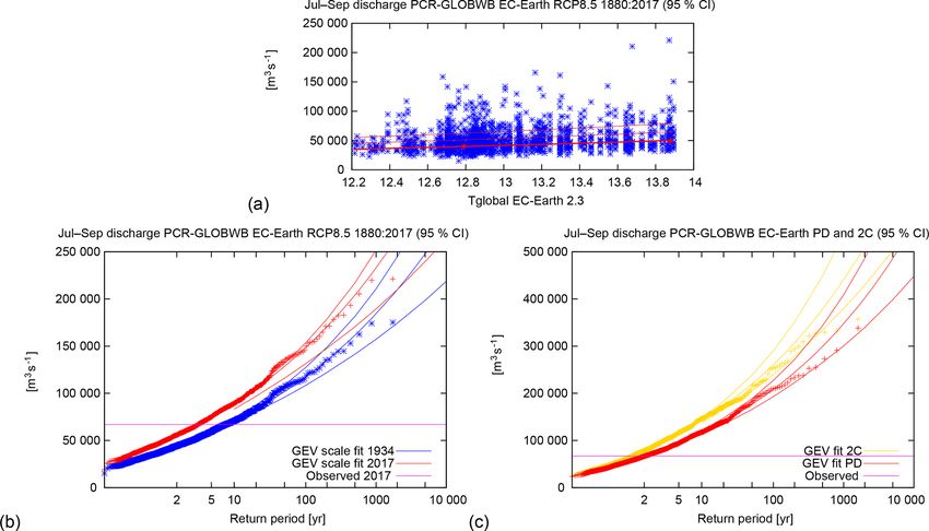
S. Philip et al.: Attributing the 2017 Bangladesh floods 1415
moisture content on temperature in the Clausius–Clapeyron uncertainty derived from each fit with the spread of the dif-
relations of about 7 % K−1 , which gives rise to an exponen- ferent estimates of the RR from observations and models. We
tial form. Note that we fit the strength of the connection, do this by computing a χ 2 /dof, with the number of degrees
which is often different from CC scaling. As it is not clear of freedom (dof) being one less than the number of fits. If
what the relevant local temperature is, but local temperature this is roughly equal to 1, the variability is compatible with
usually scales linearly with the global mean temperature, we only the natural variability that determines the uncertainty on
chose the GMST. each separate model estimate of the RR. If it is much larger
The second step in an attribution analysis is the attribution than 1, the systematic differences between the framings and
of the detected trend to global warming, natural variability models contribute significantly.
or other factors, such as changes in aerosol concentration or We choose to use a weighted average, with the weights
the El Niño–Southern Oscillation; this requires comparing being the inverse uncertainty squared for each RR (mod-
model simulations with and without anthropogenic forcing. els and observations). The uncertainties are approximated
There are two approaches. The first is to run two ensem- by symmetric
q errors on log(RR) and added in quadrature
bles: one with current conditions and one with conditions as ( 2 = 12 + 22 + . . . + N
2 /N ). If there is a significant con-
they would have been without anthropogenic emissions. The
number of events above the threshold is compared between tribution of χ 2 due to model spread, this has to be propagated
the two ensembles. In the second approach, we approximate to the final result, and the final uncertainty is larger than the
the counterfactual climate by the climate of the late 19th cen- spread due to natural variability. In this case we choose to
tury and fit the same non-stationary GEV that was described give all models equal weight. The method described here was
above to the model data. The distribution is evaluated for also used in Eden et al. (2016) and Philip et al. (2018).
a GMST in the past and the current GMST. These two ap-
proaches have been used before for studies of extreme pre-
cipitation (e.g. Schaller et al., 2014; van Oldenborgh et al., 3 Observational analysis
2016; van der Wiel et al., 2017; van Oldenborgh et al., 2017).
We checked that year-on-year autocorrelations of RX10day 3.1 Precipitation
(maximum 10-day precipitation amount) are negligible, so
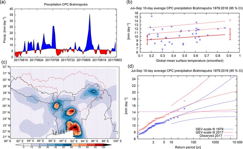
serial autocorrelations are not a problem in this analysis. Figure 3a shows the time series of CPC precipitation av-
As a third step, we calculate the risk ratio (RR) or change eraged over the Brahmaputra basin for 90 days ending on
in probability for different time intervals. These include for 2 September 2017. The 10-day average at the beginning of
instance the difference between the present day and 1979, or July is slightly higher than the 10-day average beginning of
between present-day and pre-industrial times. For observa- August, 14.38 versus 14.20 mm. As we are interested in the
tions we calculate risk ratios with respect to the beginning of August flooding event, we take the precipitation value from
the dataset. If possible, we additionally transform these into the August event, which has a maximum on 5–14 August (see
risk ratios with respect to pre-industrial conditions, in this Fig. 3c). The 10-day average annual maximum precipitation
case set to be the year 1900, such that we can compare this is fitted to a GEV distribution. The return period plots show
with model runs for pre-industrial settings. For this transfor- that the distribution can be described by a GEV by overlay-
mation we assume that the RR depends exponentially on the ing the data points and fit for the present and a past climate
covariate, in this case the global mean temperature change. (Fig. 3d). The return period calculated from this fit is 11 years
For instance if we find that the probability doubles for 0.5 ◦ C (95 % CI – confidence interval, 4 to 200 years) for the cur-
warming, we assume that first ordering it would cause it to rent climate. There is a positive trend with a risk ratio with
double again for 1 ◦ C warming. With future model runs we respect to 1979 of a factor of 6 (> 0.3), although the trend is
can also calculate risk ratios between the +2 ◦ C climate and not significant at p < 0.05 when two-sided (the uncertainty
the climate now. range includes 1).
A last step in the analysis is the synthesis of the results into A similar approach to the one used for CPC data is applied
a single attribution statement. Though the method for evalu- to ERA-int data. In this dataset the July 2017 10-day average
ating risk ratios using a transient model or observations is dif- was also just slightly higher than the August 2017 10-day av-
ferent from that using ensemble time-slice experiments that erage. The return period for the August event with a value of
are explicitly designed to simulate a +2.0 ◦ C world, we are 17.9 mm day−1 was 2 years (95 % CI, 1 to 6 years) in the cur-
able to give an average value for all observations and models rent climate. This dataset also shows a non-significant posi-
combined, and we assume that this gives a good first-order tive trend with a risk ratio of 1.9 (0.6 to 7), i.e. doubling the
estimate of the overall risk ratio. probability of an event like this or higher.
The differences among the RRs of these ensembles and Finally, the shorter GPCC dataset gives similar results as
the observations are due to natural variability, different fram- well. Risk ratios are given with respect to 1979 in order to
ings and model spread. The relative contribution of random compare this with the other datasets. The August 2017 10-
natural variability can be estimated from a comparison of the day average is slightly higher than the July 10-day average.
www.hydrol-earth-syst-sci.net/23/1409/2019/ Hydrol. Earth Syst. Sci., 23, 1409–1429, 2019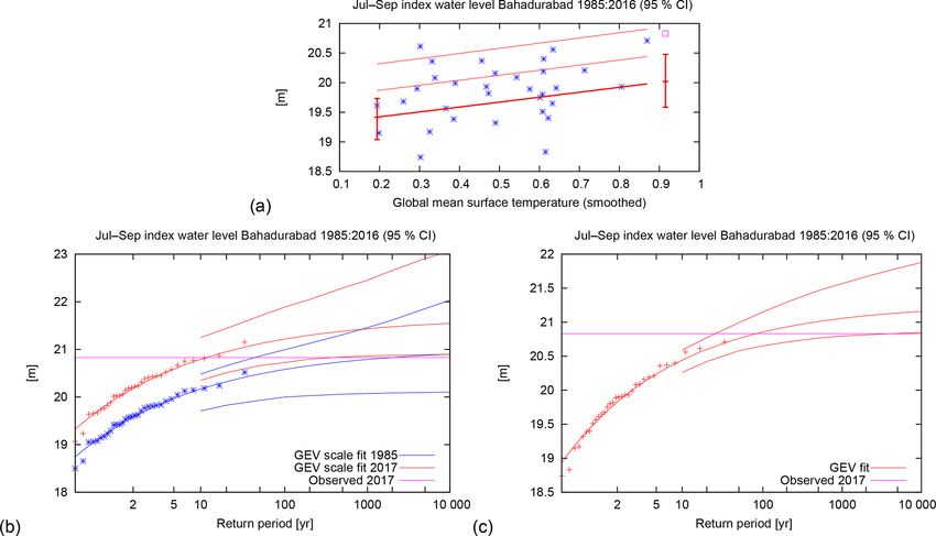
1416                                                                         S. Philip et al.: Attributing the 2017 Bangladesh floods

Figure 3. CPC data (a, c) and analysis of the highest observed 10-day mean rainfall in the Brahmaputra basin in July–September (b, d).
(a) Time series of precipitation averaged over the Brahmaputra basin; blue is more than average, and red is less than average. (b) The
location parameter µ (thick line), µ + σ and µ + 2σ (thin lines) of the GEV fit of the 10-day averaged data. The vertical bars indicate the
95 % confidence interval on the location parameter µ at the two reference years, 2017 and 1950. The purple square denotes the value of 2017
(not included in the fit). (c) The 10-day averaged precipitation over the Brahmaputra basin. Dark red means heavy precipitation. In red are the
contours of the Brahmaputra basin. (d) The GEV fit of the 10-day averaged data in 2017 (red lines) and 1950 (blue lines). The observations
are drawn twice, scaled up with the trend (smoothed global mean temperature) to 2017 and scaled down to 1950. The purple line shows the
observed value in 2017.

The return period is about 20 years (95 % CI, 4 to 800 years).            a large uncertainty in the accuracy of the discharge measure-
The risk ratio is not significantly different from 1.                     ments from 2012 onwards. We check if the results are robust
   The results of return periods and risk ratios based on ob-             by comparing the outcomes from the different datasets.
servations can be found in Table 2. For analyses with models                 We fitted the discharge time series of Bahadurabad to
we use the return period from the CPC dataset of 11 years                 a GEV distribution. In this distribution we see no trend
for this event, as based on local experience we think that this           (95 % CI with respect to – wrt – 1900 is 0.1 to 40; see Fig. 4).
is the best estimate. Due to the shape parameter being close              Therefore we calculate the return period assuming no trend.
to zero the risk ratio will not have a strong dependence on               This results in a return period of the August 2017 event of
this choice; for a Gumbel distribution it is independent of the           4 years (95 % CI, 3 to 6 years). A cross-check with the 1956–
return time.                                                              2006 dataset or merging the two discharge datasets gives sim-
                                                                          ilar results.
3.2    Discharge
                                                                          3.3   Water level
The highest discharge in 2017 was reached on 16 August,
with a value of about 78 000 m3 s−1 . This was clearly higher             Although we only have the water level available in observa-
than any value in July in the same year, as opposed to the                tions and not for models, we still analyse the observational
precipitation values discussed above. There have been sev-                water level time series from Bahadurabad. The highest value
eral years in which the discharge was higher than in 2017,                in 2017 was on 16 August, with a value of 20.83 m. This is
including the years 1998 and 1988, which are the two maxi-                1.33 m higher than the dangerous level of 19.50 m. In con-
mum values in the discharge record. The return period is cal-             trast to the discharge this was a record level since the begin-
culated from the discharge dataset since this is our best ob-             ning of the dataset (1985). It should be noted that the water
servational estimate. However it is worth noting that there is            level is also influenced by factors other than climate change,

Hydrol. Earth Syst. Sci., 23, 1409–1429, 2019                                            www.hydrol-earth-syst-sci.net/23/1409/2019/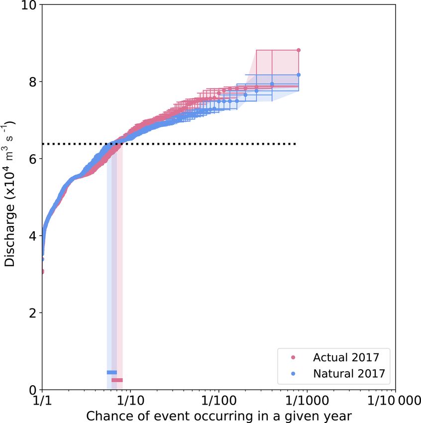
S. Philip et al.: Attributing the 2017 Bangladesh floods 1417
Table 2. Return periods and risk ratios for observations of precipitation, discharge and water level. The column RR1 gives results wrt 1979
(precipitation), 1984 (discharge) and 1985 (water level). The column RR (wrt 1900) scales the results to the pre-industrial period.
Variable Dataset (August 2017 value RT 95 % CI RR1 95 % CI RR 95 % CI
mm day−1 ) (wrt 1900)
Precipitation CPC (14.20) 11.2 4.1 to 200 6.0 > 0.30 18 > 0.2
ERA-int (17.89) 2.4 1.4 to 6.2 1.9 0.64 to 7.2 2.8 0.5 to 24
GPCC 1988–2017 (16.79) 21 4.2 to 800 0.65 0.009 to 30 0.5 0.004 to 800
Discharge 1984–2017 (78.262) 4 3 to 6 1.3 0.1 to 9 0.8 0.02 to 8
Water level 1985–2017 (20.83) 12 3 to 350 170 > 0.6
Figure 4. Analysis of the highest observed daily discharge at Bahadurabad in July–September. (a) The location parameter µ (thick line),
µ + σ and µ + 2σ (thin lines) of the GEV fit of the discharge data. The vertical bars indicate the 95 % confidence interval on the location
parameter µ at the two reference years, 2017 and 1984. The purple square denotes the value of 2017 (not included in the fit). (b) The GEV
fit of the discharge data, assuming no trend. The purple line shows the observed value in 2017.
for instance a raising of the river bed by sedimentation and For validation of the EC-Earth 2.3 model we use the years
obstruction of the river channel by man-made constructions. in the transient runs that correspond to the observational
See Sect. 6 for a more detailed discussion on the disentan- years 1979–2017. In the model, as expected, most precipi-
gling of geomorphological changes and climate change. tation falls in the months JJA, with a peak in July, like in
Under the same assumption as that for precipitation and observations, though the increase in precipitation is slightly
discharge in which water level scales with GMST, the re- stronger in June than it is in observations (Fig. S1). As it is
turn period in the current climate is estimated to be 12 years assumed that the scale parameter σ scales with the position
(95 % CI, 3 to 350 years; see Fig. 5b). However, although parameter µ of the GEV fit, we check whether the disper-
the risk ratio between 2017 and 1985 is as large as 170, sion parameter σ/µ and the shape parameter in this model
this is only non-significant with a lower bound of 0.6. This are similar to those calculated from observations. The pa-
is probably due to the relatively short length of the dataset. rameters of the GEV distribution that is fitted from the pre-
In addition, we calculate a return period assuming no trend cipitation of these model years correspond well to the same
(see Fig. 5c). This gives a return period of about 80 years parameters for CPC data.
(> 25 years, 95 % CI). This agrees with the estimates from The risk ratio of precipitation is calculated in the same
BWDB. way as that for observations, using the data period 1880–
2017 such that we can use the same years for the EC-Earth
runs and the PCR-GLOBWB and SWAT runs with EC-Earth
4 Model analysis input (see Fig. 6). The threshold is chosen such that the re-
turn period in the current climate is similar to the observed
4.1 Precipitation
return period when using the same years. The risk ratio be-
In this section we present model validation and analysis re- tween 2017 and pre-industrial conditions is 3.3 (95 % CI, 2.7
sults for the precipitation experiments, first for EC-Earth and to 4.2) in these transient runs. This corresponds to an increase
then for weather@home. in intensity for the same return period of 10 % (95 % CI, 9 %
to 11 %). For the future (figures not shown) we calculate re-
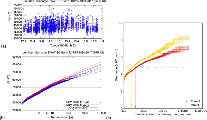
www.hydrol-earth-syst-sci.net/23/1409/2019/ Hydrol. Earth Syst. Sci., 23, 1409–1429, 20191418 S. Philip et al.: Attributing the 2017 Bangladesh floods Figure 5. Analysis of the highest observed daily water level at Bahadurabad in July–September. (a) The location parameter µ (thick line), µ + σ and µ + 2σ (thin lines) of the GEV fit of the discharge data. The vertical bars indicate the 95 % confidence interval on the location parameter µ at the two reference years, 2017 and 1985. The purple square denotes the value of 2017 (not included in the fit). (b) The GEV fit of the water level data in 2017 (red lines) and 1985 (blue lines), assuming a trend. The observations are drawn twice, scaled up with the trend (smoothed global mean temperature) to 2017 and scaled down to 1985. (c) The GEV fit of the same discharge data assuming no trend. The purple line in (b) and (c) shows the observed value in 2017. turn periods from the present and future distributions sepa- tions, see also Table 3. The threshold used in this analysis rately, again following the same statistical method as that for is defined by taking the magnitude from the historical sim- observations but with two separate GEV fits that do not de- ulation corresponding to the return period derived from the pend on the GMST. The risk ratio between a 2 ◦ C climate CPC observational dataset. and the present climate follows from this, with a value of Figure 7a shows the results for the historical and 2017- 1.8 (95 % CI, 1.7 to 2.1). We thus conclude that in the EC- specific experiments, which we use to analyse how proba- Earth 2.3 model there is a significant positive trend in the bilities may have changed in the period from pre-industrial magnitude of precipitation events such as the one in August times up until now. There is no statistically significant differ- 2017, both in the past (pre-industrial times up until now) and ence between the historical and natural simulations, with a in the future. risk ratio of 0.92 (0.84to1.02). For weather@home, we compare the annual cycle of 10- The difference in return periods between the historical and day running mean precipitation (see Fig. S2) and its spatial actual 2017 experiments gives an indication of the influence pattern in the Brahmaputra basin from historical simulations of the natural variability of the sea surface temperature (SST) with CPC and GPCC observational records. As has also been pattern in the precipitation in this region. The historical en- seen in other regions of Bangladesh (Rimi et al., 2019a), semble is driven by 30 years of differing SST patterns con- weather@home rainfall is too intense in the pre-monsoon taining different patterns of natural variability such as the El season but lies within observational uncertainty during the Niño–Southern Oscillation, whereas actual 2017 uses only monsoon season itself. Also the variability of 10-day model the observed 2017 Operational Sea Surface Temperature and precipitation is under-represented by the model for the mon- Sea Ice Analysis (OSTIA) SSTs. The SST pattern in 2017 soon season. During the monsoon season the spatial pattern (actual 2017) made extreme precipitation events less likely and magnitude of weather@home output agrees well with than the climatological mean (historical) with a risk ratio of GPCC and CPC observations (not shown). 0.25 (95 % CI, 0.2 to 0.31). Within the set of simulations Figure 7 shows the return periods of the maximum 10-day conditioned on 2017 SSTs, the negligible anthropogenic in- precipitation during JAS from the weather@home simula- fluence found in the full range SST set is confirmed; the ac- Hydrol. Earth Syst. Sci., 23, 1409–1429, 2019 www.hydrol-earth-syst-sci.net/23/1409/2019/
S. Philip et al.: Attributing the 2017 Bangladesh floods                                                                               1419

Figure 6. Analysis of the highest 10-day average precipitation in July–September in the EC-Earth model in the years 1880–2017. (a) The
location parameter µ (thick line), µ + σ and µ + 2σ (thin lines) of the GEV fit of the discharge data. The vertical bars indicate the 95 %
confidence interval on the location parameter µ at the two reference years 2017 and 1934. (b) the GEV fit of the precipitation data in
2017 (red lines) and 1934 (blue lines), assuming a trend. The data are drawn twice, scaled up with the trend (smoothed global mean model
temperature) to 2017 and scaled down to 1934. (c) GEV fits for the present day (PD, red) and +2 ◦ C world (2C, yellow) simulations. The
purple lines in (b) and (c) show the threshold value for which the risk ratio is calculated.

Figure 7. Return times of the maximum 10-day precipitation from weather@home simulations. (a) shows results from the historical, natural,
GHG-only and actual 2017, natural 2017, and GHG-only 2017 simulations, and (b) shows the historical, current, 1.5 and 2◦ simulations.
Black horizontal lines represent the threshold values derived from the CPC observations. Shaded coloured vertical boxes with solid horizontal
lines represent the uncertainty in the return period for the CPC threshold.

www.hydrol-earth-syst-sci.net/23/1409/2019/                                            Hydrol. Earth Syst. Sci., 23, 1409–1429, 2019
1420                                                                 S. Philip et al.: Attributing the 2017 Bangladesh floods

tual 2017 and natural 2017 ensembles also do not show a sta-          The runs with the PCR-GLOBWB model are treated in the
tistically significant difference and have a risk ratio of 0.97    same way as the EC-Earth runs. The experiment in which
(95 % CI, 0.76 to 1.23), indicating that, if anything, high-       the PCR-GLOBWB model is driven by CPC precipitation
precipitation events similar to the amplitude observed are         and ERA temperature and evapotranspiration shows a strong
more prevalent in our model in the natural ensemble, whether       trend in discharge, which was not seen in the discharge ob-
or not conditioned on 2017 SST conditions.                         servations. The GEV-fit parameters encompass the best es-
   To understand this result more fully it is useful to look at    timate from observations when fitted with a trend. However
the “GHG-only” simulations in Fig. 7a (compare GHG-only            the large discharge events of 1988 and 1998 are not captured
with historical simulations and GHG-only 2017 with actual          in this run (not shown).
2017 simulations). The GHG-only simulations show that in-             The experiment with ERA input, in contrast, shows no
creased GHG emissions have increased the likelihood of this        trend but clearly shows the strong discharge events of 1988
kind of event (relative to the natural simulations) but that       and 1998 (not shown). The best estimate of the GEV-fit pa-
when the sulfate aerosol emissions are taken into account (in      rameter is outside the error margins of the GEV-fit parame-
the historical and actual 2017 simulations), we find a coun-       ters of observations; however, the error margins overlap.
terbalancing effect that acts to reduce rainfall, hence reduc-        These two model runs show that the PCR-GLOBWB
ing the risk for severe flooding. This effect has also been        model is able to capture historical flood events, but the mag-
noted by van Oldenborgh et al. (2016); Rimi et al. (2018b).        nitude of these events is dependent on the meteorological in-
Within the weather@home model sulfate emissions are in-            put data. Furthermore, we find that the statistical properties
cluded, although emissions due to other important aerosols         are a fair representation of the statistical properties of ob-
such as black carbon, which can counteract sulfate effects,        served discharge.
are not represented. The aerosol effect in HadRM3P is there-          We perform an additional validation of the transient PCR-
fore potentially overestimated. The results highlight the non-     GLOBWB run with EC-Earth 2.3 input over the years cor-
linear change in risk over time as a function of anthropogenic     responding to years with observed discharge. With this input
aerosol emissions. EC-Earth follows the historical+RCP8.5          the modelled discharge peaks in August but is also high in
protocol for aerosols and includes both sulfate emissions and      July and September. We thus use the same months JAS as
black and organic carbon. It does not include any indirect         in observations for further analysis. Different from the ob-
aerosol effects. The differences in aerosol representation and     served distribution, the shape parameter ξ is positive, show-
model handling of aerosols, as well as the influence of the ex-    ing higher discharge values in the tail. This is not a prob-
perimental configuration on aerosol concentration, between         lem for this analysis, as the return period of about 4 years
EC-Earth and weather@home may account for the difference           that we are interested in is not in the tail of the distribution.
in risk ratios for the past climate period (pre-industrial times   When comparing the error margins of the ratio σ/µ with ob-
up until now) between the two models, whereas the change           served statistics we note that the model variability is too large
in risk of future climate scenarios show good agreement.           compared to the model mean. This is not the ideal situation,
   Figure 7b shows return periods from the historical, cur-        and we note in the discussion how this model bias affects the
rent, natural, 1.5 and 2.0◦ simulations, which we use to anal-     analysis.
yse how probabilities may change in the future with respect           Using the transient model runs, the risk ratio of discharge
to now. The current and historical ensembles are very similar      is calculated in the same way as that for observations, using
as expected as both are forcing simulations of differing (but      all data between 1880–2017. The risk ratio between 2017 and
overlapping) lengths. Under 1.5 and 2 ◦ C of additional warm-      pre-industrial times is 2.3 (95 % CI, 1.7 to 2.4; see Fig. 8).
ing, high precipitation within the region is set to increase       For the future we calculate return periods from the present
with risk ratios (compared to current simulation) derived us-      and future distributions separately, following the same sta-
ing the CPC observational threshold of 1.46 (95 % CI, 1.27         tistical method as that for precipitation in the EC-Earth 2.3
to 1.69) and 1.74 (95 % CI, 1.52 to 1.99) respectively. In both    present and future experiments. The risk ratio between a 2 ◦ C
cases the ERA-int (GPCC) threshold risk ratio is smaller           climate and the present follows from this, with a value of
(larger) than the CPC threshold risk ratio (not shown), but        1.3 (95 % CI, 1.2 to 1.4). We thus conclude that in the PCR-
with overlapping uncertainty bounds with CPC. For 2 ◦ C of         GLOBWB model driven by EC-Earth output there is a posi-
warming these risk ratios show good agreement with the EC-         tive trend in discharge events like the one in August 2017 in
Earth values.                                                      both the historical period (pre-industrial times to 2017) and
                                                                   the future period (from current conditions to a +2 ◦ C world).
                                                                      The SWAT model calibrated with EC-Earth meteorologi-
4.2    Discharge
                                                                   cal data tends to underestimate flows in almost all months of
                                                                   the year (see Fig. S3 in the Supplement). The SWAT model
In this section we present model validation and results of the     calibrated with weather@home meteorological data, in con-
discharge simulations, first for the model PCR-GLOBWB              trast, tends to underestimate flows in the monsoon months
and then for SWAT, LISFLOOD and the RFM.                           while overestimating flows in the remaining months. There-

Hydrol. Earth Syst. Sci., 23, 1409–1429, 2019                                    www.hydrol-earth-syst-sci.net/23/1409/2019/
S. Philip et al.: Attributing the 2017 Bangladesh floods 1421
Table 3. Risk ratios for precipitation and discharge for models and observations for both present to pre-industrial times or 1900 and a 2 ◦ C
climate to present. 95 % confidence intervals are given as well.
Dataset RR (present / pre- 95 % CI RR (2◦ C 95 % CI
industrial or 1900) / present)
Precipitation CPC 18.2 > 0.20
EC-Earth 2.3 3.27 2.65 to 4.24 1.81 1.75 to 2.14
W@h (historical / natural) 0.92 0.84 to 1.02 1.74 1.52 to 1.99
W@h (GHG only / natural) 1.73 1.34 to 2.25
W@h (GHG only / historical) 1.35 1.23 to 1.49
W@h (actual 2017 / natural 2017) 0.97 0.76 to 1.23
W@h (GHG only 2017 / natural 2017) 1.65 1.38 to 1.96
W@h (GHG only / actual 2017) 1.69 1.35 to 2.13
Discharge Observations 1.43 0.05 to 42.5
PCR-GLOBWB (EC-Earth) 2.34 1.74 to 2.37 1.34 1.23 to 1.41
SWAT – EC-Earth (transient) 1.49 1.30 to 1.57 1.56 1.45 to 1.7
SWAT – W@h (actual 2017 / natural 2017) 0.88 0.72 to 1.09
LISFLOOD – W@h (actual 2017 / natural 2017) 1.35 1.20 to 1.51
LISFLOOD – W@h (GHG only 2017 / actual 2017) 1.29 1.10 to 1.45
LISFLOOD – W@h (GHG only 2017 / natural 2017) 1.74 1.52 to 2.01
RFM – W@h (actual 2017 / natural 2017) 1.13 1.11 to 1.14
RFM – W@h (GHG only 2017 / actual 2017) 1.53 1.50 to 1.56
RFM – W@h (GHG only 2017 / natural 2017) 1.73 1.71 to 1.74
Figure 8. Analysis of the highest discharge at Bahadurabad in July–September in the PCR-GLOBWB model in the years 1920–2017. (a) The
location parameter µ (thick line), µ + σ and µ + 2σ (thin lines) of the GEV fit of the discharge data. The vertical bars indicate the 95 %
confidence interval on the location parameter µ at the two reference years 2017 and 1934. (b) The GEV fit of the discharge data in 2017 (red
lines) and 1934 (blue lines), assuming a trend. The observations are drawn twice, scaled up with the trend (smoothed global mean model
temperature) to 2017 and scaled down to 1934. (c) GEV fits for the present day (PD, red) and +2 ◦ C world (2C, yellow) simulations. The
purple horizontal lines in (b) and (c) show the threshold value for which the risk ratio is calculated.
www.hydrol-earth-syst-sci.net/23/1409/2019/ Hydrol. Earth Syst. Sci., 23, 1409–1429, 20191422 S. Philip et al.: Attributing the 2017 Bangladesh floods
fore in both cases, flows in our months of interest (JAS) are more frequent in the region if the air pollution levels are re-
always slightly underestimated, but the magnitudes of error duced in the future.
appear limited enough for the models to be useful in conduct- The risk ratios for the observed threshold from both LIS-
ing attribution studies. When comparing the error margins of FLOOD and the RFM of 1.35 (95 % CI, 1.20 to 1.51) and
the ratio σ/µ with observed statistics we note that the model 1.13 (95 % CI, 1.11 to 1.14) respectively are in good agree-
variability is too small compared to the model mean, opposite ment even though the simulated river flows by the models
to what was found for the PCR-GLOBWB model. The shape are different. The mitigation effect due to the aerosols is also
parameter ξ is of the same order as the one in the observed comparable between these two different hydrological mod-
discharge dataset. els.
The risk ratios are calculated from return period plots for
both the EC-Earth runs (see Fig. 9) and the weather@home
runs (see Fig. 10). Using the SWAT model runs with EC- 5 Synthesis
Earth transient data, we see that the discharge shows some
decadal variability. The trend in the data therefore depends In observations the uncertainties in return periods and risk ra-
more strongly on the years used. For consistency we use tios are quite large. This is mainly due to the shorter lengths
the same years as in the analyses of EC-Earth and PCR- of the time series, and natural variability dominates. In the
GLOBWB data (1880–2017), and we note that the error mar- models, the signal-to-noise ratio is much larger, resulting
gins do not capture this variability and are underestimated. in smaller uncertainties in the risk ratios. Here, the model
The risk ratio of discharge between 2017 and pre-industrial spread dominates the signal. As both natural variability and
times is found to be 1.5 (95 % CI, 1.3 to 1.6). The risk ra- model spread play a role, we use a weighted average with
tio between a 2 ◦ C climate and the current climate is 1.56 inflated uncertainty range. We do not synthesize the risk ra-
(95 % CI, 1.45 to 1.70). Using the SWAT model runs with tios for the future, as we only have two model estimates per
weather@home actual 2017 and natural 2017 data, the risk variable.
ratio between the actual 2017 and natural 2017 scenario is In the synthesis we use all available observational datasets
0.88 (95 % CI, 0.72 to 1.09). that are analysed in this paper and one experiment per model.
Calibration and validation graphs for LISFLOOD and the For weather@home and all hydrological models that use in-
RFM are shown in the Supplement. They show that both LIS- put from weather@home experiments we use the risk ra-
FLOOD and RFM are able to simulate the seasonality of rise tios calculated from the actual 2017 and natural 2017 ex-
in spring and summer flows correctly. Both models underesti- periments. This gives us a fair opportunity to compare the
mate the river discharge in summer, with an underestimation synthesis of precipitation with the synthesis of discharge.
in the simulated discharge by LISFLOOD. The synthesis results are shown in Fig. 12. The synthesis
The return period and risk ratio for the LISFLOOD model of the precipitation analysis results in a risk ratio between
and RFM estimated from the weather@home actual 2017 2017 and pre-industrial times of 1.8 (95 % CI, 0.5 to 9.3).
and natural 2017 datasets, as well as the results for the GHG- Although the best estimate is above 1, the trend is not signif-
only 2017 runs, are shown in Fig. 11. icant due to the relatively large error margins. The synthesis
The LISFLOOD model shows that a discharge value with of the discharge analysis results in a risk ratio between 2017
a return period of 4 years in the actual scenario would in- and pre-industrial times of 1.1 (95 % CI, 1.0 to 1.3). So for
crease to 5.4 years in the natural climate scenario (risk ratio discharge the best estimate is only slightly higher than 1, and
of 1.35 – 95 % CI, 1.20 to 1.51), while it would reduce to due to the smaller error margins in the average, this trend is
3.1 years in the GHG-only scenario. only significant under the assumptions made in this analysis.
The trend is similar in the results simulated by the RFM,
however, the discharge value with a return period of 4 years
is slightly greater than the value simulated by LISFLOOD. 6 Discussion
The return period would increase to 4.5 years under natural
climate conditions (risk ratio of 1.13 – 95 % CI, 1.11 to 1.14), In any event-attribution study, tasks to be carried out include
while it would reduce to 2.6 years in the GHG-only scenario. the following:
Note however that from Fig. 11b we see that the risk ratio
between the different scenarios for RFM becomes larger for i. determining what happened using available observa-
larger return periods (e.g. 10 years) than those studied in this tions and defining the event to be studied,
analysis.
The shorter return period in the GHG-only 2017 scenario ii. determining how rare the event is in current and pre-
shows that if sulfate aerosols are removed from the atmo- industrial conditions,
sphere (which results in increased precipitation), flooding be-
comes more frequent. This implies that floods can become iii. using models to attribute any changes in likelihood of
similar classes of events.
Hydrol. Earth Syst. Sci., 23, 1409–1429, 2019 www.hydrol-earth-syst-sci.net/23/1409/2019/You can also read