WRF4PALM v1.0: a mesoscale dynamical driver for the microscale PALM model system 6.0
←
→
Page content transcription
If your browser does not render page correctly, please read the page content below
Geosci. Model Dev., 14, 2503–2524, 2021
https://doi.org/10.5194/gmd-14-2503-2021
© Author(s) 2021. This work is distributed under
the Creative Commons Attribution 4.0 License.

WRF4PALM v1.0: a mesoscale dynamical driver for the microscale
PALM model system 6.0
Dongqi Lin1,2 , Basit Khan3 , Marwan Katurji2 , Leroy Bird4 , Ricardo Faria5 , and Laura E. Revell1
1 School  of Physical and Chemical Sciences, University of Canterbury, Christchurch, New Zealand
2 School  of Earth and Environment, University of Canterbury, Christchurch, New Zealand
3 Institute of Meteorology and Climate Research, Atmospheric Environmental Research (IMK-IFU),

Karlsruhe Institute of Technology (KIT), 82467 Garmisch-Partenkirchen, Germany
4 Bodeker Scientific, Alexandra, New Zealand
5 Oceanic Observatory of Madeira, Agência Regional para o Desenvolvimento da Investigação Tecnologia e Investigação,

Madeira, Portugal

Correspondence: Dongqi Lin (dongqi.lin@pg.canterbury.ac.nz)

Received: 13 September 2020 – Discussion started: 1 December 2020
Revised: 1 March 2021 – Accepted: 14 March 2021 – Published: 6 May 2021

Abstract. A set of Python-based tools, WRF4PALM, has          ing from WRF outputs. The WRF4PALM tools presented
been developed for offline nesting of the PALM model          here can potentially be used for micro- and mesoscale studies
system 6.0 into the Weather Research and Forecasting          worldwide, for example in boundary layer studies, air pol-
(WRF) modelling system. Time-dependent boundary con-          lution dispersion modelling, wildfire emissions and spread,
ditions of the atmosphere are critical for accurate repre-    urban weather forecasting, and agricultural meteorology.
sentation of microscale meteorological dynamics in high-
resolution real-data simulations. WRF4PALM generates ini-
tial and boundary conditions from WRF outputs to pro-
vide time-varying meteorological forcing for PALM. The        1   Introduction
WRF model has been used across the atmospheric sci-
ence community for a broad range of multidisciplinary ap-     Over the last decade, research in numerical weather and cli-
plications. The PALM model system 6.0 is a turbulence-        mate simulations, environmental modelling, and agricultural
resolving large-eddy simulation model with an additional      and urban meteorology has developed to include higher spa-
Reynolds-averaged Navier–Stokes (RANS) mode for atmo-         tial resolutions, such that the feedback from the microscale
spheric and oceanic boundary layer studies at microscale      (from 10−2 to 103 m; from seconds to hours) processes im-
(Maronga et al., 2020). Currently PALM has the capabil-       pacted by surface heterogeneities can be explicitly resolved
ity to ingest output from the regional scale Consortium       and better represented. At the mesoscale (from 104 to 5 ×
for Small-scale Modelling (COSMO) atmospheric predic-         105 m; from hours to days), numerical weather prediction
tion model. However, COSMO is not an open source model        (NWP) models are widely used to simulate regional atmo-
and requires a licence agreement for operational use or       spheric flows in real meteorological conditions. Mesoscale
academic research (http://www.cosmo-model.org/, last ac-      NWP models are primarily Reynolds-averaged (Navier–
cess: 23 April 2021). This paper describes and validates      Stokes) (RANS) simulation models that parameterise tur-
the new free and open-source WRF4PALM tools (available        bulence without discrepancy for scale (Sagaut, 2006, Chap-
at https://github.com/dongqi-DQ/WRF4PALM, last access:        ter 1.4). The parameterisations applied in RANS models only
23 April 2021). Two case studies using WRF4PALM are pre-      consider the average properties of atmospheric flows im-
sented for Christchurch, New Zealand, which demonstrate       pacted by surface geometries at the grid resolution of the
successful PALM simulations driven by meteorological forc-    simulation. In contrast to RANS models, large-eddy simu-
                                                              lation (LES) models apply a local spatial filter to solve 3-

Published by Copernicus Publications on behalf of the European Geosciences Union.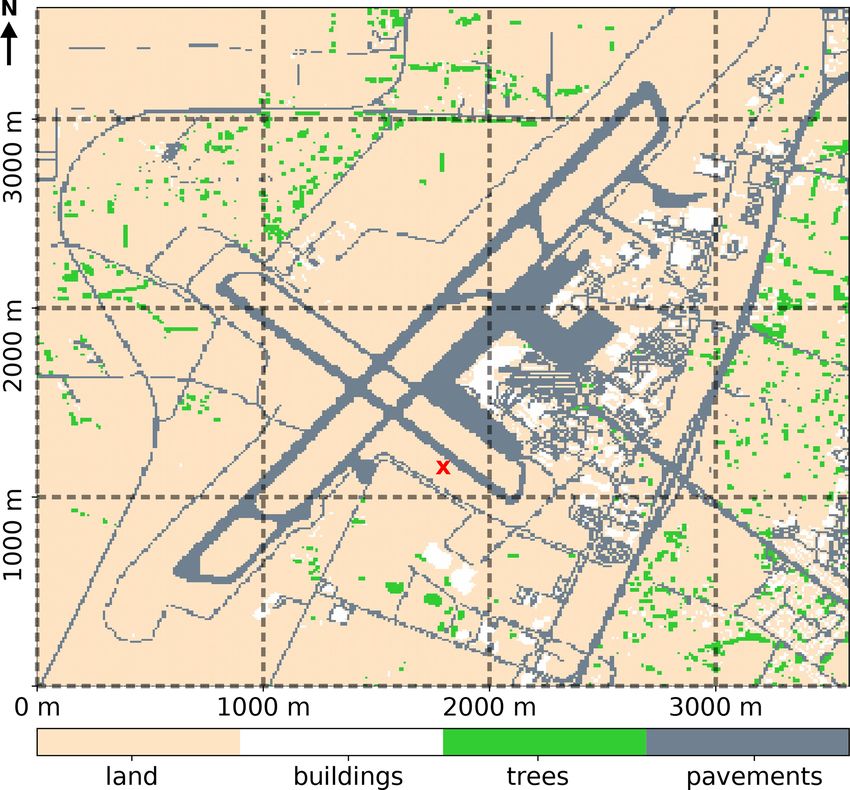
2504                                                                                                D. Lin et al.: WRF4PALM

D prognostic equations (Sagaut, 2006, Chapter 1.4). Eddies        dauf et al., 2007). Vollmer et al. (2015) successfully used
with scales smaller than the filter (sub-grid scales) are pa-     COSMO and PALM to reproduce an offshore wind turbine
rameterised while eddies larger than the filter are termed as     wake in Germany. However, at present, the COSMO model
large eddies and are resolved explicitly. LES models have         is not an open-source model and therefore cannot be di-
been used to simulate and understand airflows around ur-          rectly applied to most regions outside of the European do-
ban canopy structures at scales of several metres (hereafter      main. Kurppa et al. (2020) used mesoscale data from Me-
fine scale). For example, Bergot et al. (2015) applied the        teorological Cooperation on Operational Numerical Weather
LES technique embedded in the non-hydrostatic anelastic re-       Prediction (MetCoOp) Ensemble Prediction System (MEPS;
search model Meso-NH to study fog life cycle and dispersion       Bengtsson et al., 2017; Müller et al., 2017), operated by
stability at fine scale, Wyszogrodzki et al. (2012) used LES-     the Norwegian Meteorological Institute, to provide realistic
EULAG to simulate fine-scale urban dispersion, and Kurppa         boundary conditions in PALM. Similar to COSMO, MEPS is
et al. (2020) used the Parallelised Large-Eddy Simulation         currently not publicly available.
Model (PALM) to analyse spatial distributions of aerosols.           To extend the use of PALM for the scientific commu-
   Although LES models are known to have better perfor-           nity, we have developed a set of Python tools to allow
mance than RANS models when addressing transport and              PALM to include mesoscale forcing from the Weather Re-
dispersion problems (Gousseau et al., 2011), mesoscale flows      search and Forecasting modelling system (WRF; http://www.
still have significant impact on the local LES scale. For sim-    wrf-model.org, last access: 23 April 2021; Skamarock et al.,
ulations to represent realistic meteorology with high fidelity,   2019). These tools are hereafter referred to as WRF4PALM,
it is essential that the effects of mesoscale flows are cap-      i.e. tools that process WRF output for use in PALM simu-
tured. Therefore, time-varying initial and boundary condi-        lations. The free open-source WRF model has been exten-
tions of the atmosphere are important to achieve realistic at-    sively used for atmospheric research and weather forecast-
mospheric simulations in LES domains. With a turbulence-          ing throughout the world (Skamarock et al., 2019). Using
and building-resolving LES model at its core, the PALM            WRF4PALM, modellers can offline nest the PALM model
model system 6.0 has been used to study atmospheric and           within the WRF model to generate simulations that resolve
oceanic boundary layers for over 20 years (Maronga et al.,        microscale meteorological dynamics.
2015, 2020). In recent years the PALM model has been ex-             This paper describes WRF4PALM and presents validation
tended by implementing PALM-4U (PALM for urban ap-                of the tools. The PALM dynamical input data standard is de-
plications) components for application of the PALM model          scribed in Sect. 2. A description of the WRF4PALM frame-
in the urban environments. (Maronga et al., 2015, 2020;           work is described in Sect. 3. Section 4 shows the validation
Heldens et al., 2020). High-resolution (fine-scale) PALM          and initial application of WRF4PALM. Section 5 presents
simulations have proven to be useful for city planners to         conclusions and an outlook for WRF4PALM.
determine the optimal layout of surface structures, such as
buildings, vegetation, and pavement, to mitigate adverse air-
quality impacts (e.g. Gronemeier et al., 2017; Kurppa et al.,     2   PALM offline nesting and dynamical input
2018, 2020). However, the studies by Gronemeier et al.
(2017) and Kurppa et al. (2018) only performed idealised          The offline nesting module embedded in PALM works as
simulations where the direction and intensity of the wind at      an interface between a mesoscale atmospheric model and
inflow were invariant during the entire simulation period. In     PALM (Maronga et al., 2020). This interface requires users
addition, their simulation domains have to be reoriented to       to provide PALM with a netCDF dynamical driver file as an
accommodate the impact of wind direction, which can lead          input (hereafter referred to as the dynamic driver to be con-
to a large amount of additional manual data processing.           sistent with PALM documentation), which contains the me-
   PALM was designed to seamlessly apply forcing from             teorological forcing and initial profiles of atmospheric state
mesoscale models in a one-way or offline nesting approach         variables extracted from the mesoscale model. The dynamic
(Maronga et al., 2015; Vollmer et al., 2015; Heinze et al.,       driver created by WRF4PALM focuses solely on correctly
2017; Maronga et al., 2020; Kadasch et al., 2020). Here           and appropriately interpolating the meteorological and sub-
one-way or offline nesting is realised as meteorological forc-    surface fields extracted from WRF to fulfil the input data re-
ings from mesoscale models are passed onto PALM, while            quirements of PALM.
PALM does not have to run along with or provide any feed-            Following the PALM Input Data Standard (PIDS) (https:
back to the mesoscale model. Currently, the PALM model            //palm.muk.uni-hannover.de/trac/wiki/doc/app/iofiles/pids,
system 6.0 provides the additional software package INI-          last access: 23 April 2021), the dynamic driver must include
FOR (Maronga et al., 2020; Kadasch et al., 2020), which           initial vertical profiles of the atmosphere and soil, the lateral
can process mesoscale data for use by PALM. However, INI-         and top boundary conditions of the atmosphere, and the
FOR is currently configured to only process data output from      time series of the surface pressure (Table 1). Note that the
the regional weather prediction model COSMO (Consortium           variables listed in Table 1 are based on PIDS v1.9. While
for Small-scale Modelling), formerly named as LM-K (Bal-          some variable names may be changed in future updates of

Geosci. Model Dev., 14, 2503–2524, 2021                                            https://doi.org/10.5194/gmd-14-2503-2021
D. Lin et al.: WRF4PALM                                                                                                        2505

Table 1. Variables in the PALM dynamic driver based on PALM input data standard v1.9.

              Variable name                                    Description
              init_soil_t                                      Initial vertical profile of soil temperature
              init_soil_m                                      Initial vertical profile of soil moisture
                                                               Initial vertical profile of X in the atmosphere as follows:
              init_atmosphere_X
                                                               X     Variable long name                       Units
                                                               pt    Potential temperature                    K
                                                               qv    Specific humidity                        kg kg−1
                                                               u     Wind component in x direction            m s−1
                                                               v     Wind component in y direction            m s−1
                                                               w     Subsidence velocity                      m s−1
              ls_forcing_left_X                                Large-scale forcing data of X for left model boundary
              ls_forcing_right_X                               Large-scale forcing data of X for right model boundary
              ls_forcing_north_X                               Large-scale forcing data of X for north model boundary
              ls_forcing_south_X                               Large-scale forcing data of X for south model boundary
              ls_forcing_ug                                    u wind component geostrophic (units: m s−1 )
              ls_forcing_vg                                    v wind component geostrophic (units: m s−1 )
              surface_forcing_surface_pressure                 Large-scale surface forcing of surface pressure (units: Pa)

Table 2. Variables used in WRF4PALM.                                    The data passed from WRF to PALM include veloc-
                                                                     ity fields, thermodynamic components (pressure, tempera-
           Variables                       Units                     ture, potential temperature, and water vapour mixing ra-
           Velocity components (u, v, w)   m s−1                     tio), soil features, vertical grid structure (geopotential), and
           Temperature                     K                         geographical information (Table 2). The code structure of
           Potential temperature           K                         WRF4PALM is shown in Fig. 1. WRF4PALM is written
           Pressure                        Pa                        in the Python3 programming language. Two major Python
           Water vapour mixing ratio       kg kg−1                   scripts comprise WRF4PALM. One is create_cfg.py,
           Soil moisture                   m3 m−3                    which reads user input and specifies the PALM domain
           Soil temperature                K                         within the WRF domain using latitude and longitude bounds.
           Perturbation geopotential       m2 m−2                    The other is create_dynamic.py, which processes
           Base-state geopotential         m2 m−2                    WRF dynamical fields to create the PALM dynamic driver.
           Latitudes and longitudes        degree                    Detailed step-by-step instructions for running WRF4PALM
                                                                     are given in Appendix B.
                                                                        The PALM grid configuration prescribes how the WRF
PALM, these can be modified in the WRF4PALM code in                  output needs to be interpolated onto the PALM grid cells
such cases.                                                          along west–east (nx), south–north (ny), and bottom–top
                                                                     (nz) coordinates and the corresponding grid spacing along
                                                                     each direction (dx, dy, and dz respectively). The lati-
                                                                     tude and longitude of the centre of the PALM domain
3     Methodology                                                    must be provided to specify the PALM domain loca-
                                                                     tion in the WRF domain. By obtaining the aforemen-
3.1    WRF4PALM framework                                            tioned domain configuration information from users, the
                                                                     create_cfg.py script then generates a configuration file
The new WRF4PALM (available on https://github.com/                   containing latitudes and longitudes for the north, south,
dongqi-DQ/WRF4PALM, last access: 23 April 2021) is                   east, and west lateral boundaries and a grid configuration
based on WRF2PALM initially developed by Faria (2019).               for the PALM domain. The configuration file then acts as
Modifications and changes made to WRF2PALM to create                 an input for create_dynamic.py to finish the interpo-
WRF4PALM are described in Appendix A.

https://doi.org/10.5194/gmd-14-2503-2021                                                  Geosci. Model Dev., 14, 2503–2524, 2021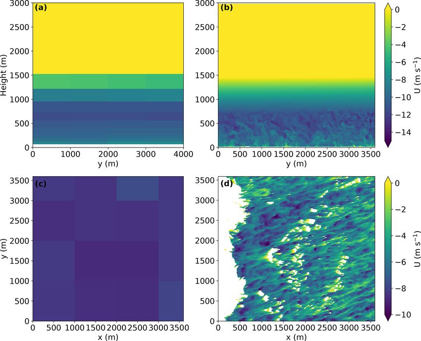
2506                                                                                                   D. Lin et al.: WRF4PALM

Figure 1. The code structure of WRF4PALM. Green boxes indicate input from users. Blue boxes indicate the Python script used. The big
yellow box illustrates the processes used to interpolate and pass WRF dynamical fields to the PALM dynamic driver. White boxes outside
the yellow box indicate output files of WRF4PALM.

lation. WRF4PALM also allows users to apply stretched                tion of WRF4PALM is the same as that described in Maronga
grid spacing along the z direction. Identical to parame-             et al. (2015).
ters used in the PALM input parameter list, users must de-              Because both PALM and WRF use the Arakawa Carte-
fine dz_stretch_level, dz_stretch_factor, and                        sian grid staggering (staggered Arakawa C-grid; Harlow and
dz_max for vertically stretched grid spacing.                        Welch, 1965; Arakawa and Lamb, 1977), no transformation
   The create_dynamic.py script requires users to pro-               is required in PALM for staggered data. After reading the in-
vide their own WRF output. WRF offers an abundance of                put parameters described above, the script first extracts WRF
choices of parameterisations for microphysics, radiation, sur-       data for the specified period and location required for PALM.
face layer, etc. Users also have a high degree of freedom to         Potential temperature, air temperature, and pressure fields
choose the meteorological data for initialisation, geospatial        are read using the getvar function embedded in the WRF-
data, and projection of the simulation domain. Although op-          Python package (Ladwig, 2019). Other variables, such as wa-
timal WRF configurations will depend on the user’s own re-           ter vapour mixing ratio and wind field, are read using the
search interests, any WRF output containing data described           xarray package (Hoyer and Hamman, 2017). Other than the
in Table 2 is considered applicable for WRF4PALM.                    vertical component of wind (w), all WRF variables are first
   PALM also requires the start and end time stamps (in              interpolated on each horizontal field from the WRF domain
YYYY, MM, DD, HH format) and lateral and top bound-                  onto the PALM horizontal Cartesian grid. The horizontal in-
ary conditions update frequency to be provided by users.             terpolation uses the SciPy package (Virtanen et al., 2020).
The lateral and top boundary conditions can update from              The WRF data that were horizontally interpolated to the
every 1 min to every 6 h (or more) depending on the tem-             PALM grid are then vertically interpolated onto the PALM
poral frequency of WRF output and the user’s own re-                 vertical Cartesian physical height levels. This requires the
search needs. The thickness of the individual soil layers            interplevel function in the WRF-Python package (Lad-
(dz_soil) to be used in PALM must be specified in                    wig, 2019), which reads the WRF physical height levels and
create_dynamic.py. The default eight-layer configura-                interpolates the given data onto required PALM vertical lev-
                                                                     els as defined in the PALM domain configuration file created

Geosci. Model Dev., 14, 2503–2524, 2021                                               https://doi.org/10.5194/gmd-14-2503-2021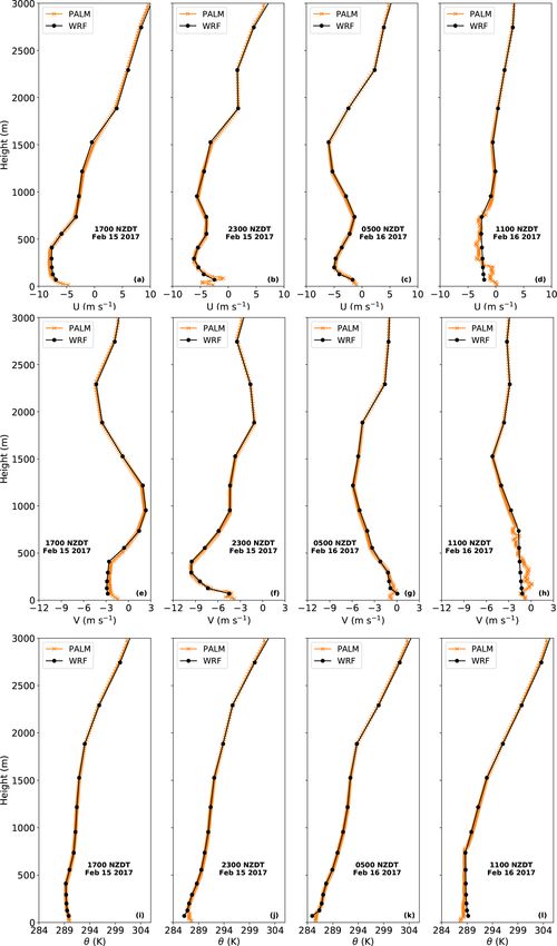
D. Lin et al.: WRF4PALM                                                                                                      2507

by create_cfg.py. The WRF physical height levels are              velocity (u and v), a logarithmic fit is applied. After solv-
calculated using                                                  ing surface NaN values, the initial vertical profiles are cal-
                                                                  culated by taking the horizontal average of velocity compo-
z = (PH + PHB)/g,                                          (1)    nents, potential temperature, and water vapour mixing ratio
where PH is the perturbation geopotential in m2 s−2 , PHB         at the initial time for each vertical level. The time series of
is the base-state geopotential, and g is gravitational acceler-   surface pressure in the dynamic driver is the time series of
ation (9.81 m2 s−2 ). Equation (1) only gives staggered ver-      horizontal average of pressure at the lowest level after inter-
tical height levels, which are then destaggered using the         polation. Soil moisture and temperature are interpolated to
destagger function in the WRF-Python package (Lad-                soil layers provided by users. Due to the difference in the
wig, 2019) for vertical interpolation of variables that are not   grid resolution and data sources between WRF and PALM,
vertically staggered. When WRF is operated under RANS             all the soil moisture for water bodies in WRF (where soil
mode, the value of the vertical component of wind (w) does        moisture is equal to 100 %) is replaced by the median value
not represent any turbulence and could be very small in           of land soil moisture in the given PALM simulation domain
WRF. These small values may lead to possible missing val-         to avoid mismatch between the PALM and WRF landmasks.
ues in the horizontal and subsequently the vertical interpo-      To take into account water bodies in PALM, a netCDF static
lation. In order to avoid this issue, the vertical component      driver input file is required (Heldens et al., 2020), where
of wind (w) from WRF is first interpolated vertically to          the types and locations of water bodies are specified. De-
PALM vertical-staggered Cartesian physical height levels us-      tails about static files used in this work are presented in
ing staggered vertical height levels calculated by Eq. (1) and    Sect. 3.2. WRF4PALM also gives the soil information at each
interplevel function in the WRF-Python package (Lad-              soil layer (soil_moisture, soil_temperature, and
wig, 2019). Then, the vertically interpolated data are inter-     deep_soil_temperature, identical to PALM input pa-
polated horizontally to the PALM horizontal Cartesian grid.       rameters), which can be added into the input parameter list of
Once all the interpolation processes of the aforementioned        the PALM land surface model. Details of algorithms applied
variables are completed, geostrophic winds are calculated as-     in WRF4PALM are provided in the online documentation of
suming geostrophic balance:                                       WRF4PALM.
                                                                     The dynamic driver of PALM generated by the
      1 1P                                                        create_dynamic.py script only contains meteorologi-
vg =       ,                                               (2)
     ρf ∂x                                                        cal and sub-surface fields from WRF and does not encom-
        1 1P                                                      pass any parameterised processes. Since turbulence is com-
ug = −       ,                                             (3)    pletely parameterised in WRF, it is also not included in the
       ρf ∂y
                                                                  dynamic driver. In order to obtain realistic flow characteris-
where ρ is air density in kg m−3 , f is the Coriolis parame-      tics, non-cyclic boundary conditions must be applied. When
ter, P is pressure, and x and y are coordinates along west–       non-cyclic boundary conditions are used with offline nest-
east and south–north respectively. Note that as commented         ing, because no turbulence is included in the inflow, either a
in the PALM 6.0 Overview (Maronga et al., 2020) and in            large domain is required to allow sufficient space and time
the PALM mesoscale nesting interface description (Kadasch         for turbulence to develop or the synthetic turbulence genera-
et al., 2020), geostrophic winds are not required in the dy-      tor (STG) must be applied (Gronemeier et al., 2015).
namic driver at present. Users can exclude the geostrophic
wind forcing by amending the WRF4PALM code them-                  3.2   PALM static driver
selves.
    The height levels in WRF are terrain following (Ska-          To resolve and realise near-surface microscale structures,
marock et al., 2019) while the Cartesian topography in            PALM can read a netCDF static driver file (hereafter static
PALM allows for explicitly resolving obstacles such as build-     driver) as an input. The static driver includes information on
ings and orography (Maronga et al., 2015). Due to such            buildings, streets, vegetation, soil, water bodies, etc., in the
differences in topography representation, the vertical inter-     model domain (Heldens et al., 2020). Due to high variability
polation can lead to Not a Number (NaN) values near the           in geospatial data availability and quality across the world,
ground surface when WRF data are vertically interpolated          there is no standard process to generate the PALM static
onto PALM vertical levels below the first WRF model level.        driver. WRF4PALM does not require users to provide a static
It would be inefficient to create NaN masks and filter data to    driver, which is applicable to both realistic simulations (with
fit the entire topography and all surface geometries in PALM      a static driver) and relatively idealised simulations (without
simulations. Hence, the surface NaN solver is applied to fill     a static driver). However, we recommend that users include
the NaN values near the surface. For all the scalar variables     the static driver in PALM simulations for more realistic and
and the vertical velocity (w), the surface NaN values are         representative results to understand the impact of microscale
filled by taking the values from the lowest level where valid     surface structures. In the case studies described later, a static
values exist at the grid point. For horizontal components of      driver is included. We adopted a similar procedure described

https://doi.org/10.5194/gmd-14-2503-2021                                            Geosci. Model Dev., 14, 2503–2524, 2021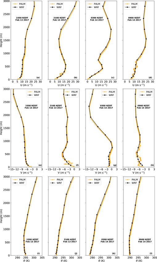
2508                                                                                             D. Lin et al.: WRF4PALM

in Heldens et al. (2020) to create the static driver. Various   physics suite (Liu et al., 2017). This physics suite includes
geospatial data sources are used including                      the microphysics parameterisation developed by Thompson
                                                                et al. (2008), the Tiedtke cumulus parameterisation (Tiedtke,
    – digital surface model (DSM) and digital elevation         1989; Zhang et al., 2011) (domains D01 and D02 only; see
      model (DEM) from Envirionment Canterbury Regional         Fig. 2; no cumulus parameterisation scheme is applied for
      Council (2020)                                            domains D03 and D04; see Fig. 2), the RRTMG models
                                                                (Iacono et al., 2008) for longwave and shortwave radiation,
    – street and pavement type information from Open-
                                                                the quasi-normal scale elimination (QNSE) planetary bound-
      StreetMap (https://planet.openstreetmap.org/, last ac-
                                                                ary layer (PBL) physics parameterisation (Sukoriansky et al.,
      cess: 18 May 2020)
                                                                2005), the eta similarity scheme (Monin and Obukhov, 1954;
    – building information from New Zealand building out-       Janjić, 1994, 1996, 2001) for surface layer parameterisa-
      lines dataset (Land Information New Zealand, 2020a)       tion, and the unified Noah land surface model (Tewari et al.,
                                                                2016). Both WRF simulations presented in this study have a
    – land cover classification data from the Land Cover        spin-up time of at least 24 h and do not have data assimilation
      Database (LCDB) version 5.0, Mainland New Zealand         technique applied.
      (Landcare Research, 2020)                                    Both of the PALM simulations described in the case stud-
                                                                ies use the following sub-models embedded in PALM: ra-
    – water bodies information from New Zealand parcels         diation model, land surface model, urban surface model,
      dataset (Land Information New Zealand, 2020b).            plant canopy model, synthetic turbulence generator, and of-
                                                                fline nesting module. Since this work only aims to demon-
                                                                strate WRF4PALM’s applicability and give an overview of
4     Case studies
                                                                WRF4PALM’s performance, the 1 km grid spacing WRF
Two case studies are presented here to demonstrate the per-     output is directly processed to 10 m grid spacing PALM.
formance, stability, and applicability of WRF4PALM. The         The time-dependent 10 m grid spacing boundary conditions
local solar time, i.e. New Zealand daylight time (NZDT), is     are stored in the dynamic driver processed by WRF4PALM.
used for both case studies presented below. Both the case       Both of the simulations use non-cyclic boundary conditions
studies were centred on Christchurch airport, New Zealand       to represent realistic meteorological conditions. STG is used
(43.4864◦ S, 172.5369◦ E). Christchurch sits in the Canter-     in this study to reduce the adjustment zone size near the
bury Plains and in the zone of mid-latitude westerlies in       boundary and to accelerate turbulence development. STG im-
the Southern Hemisphere. A succession of subtropical an-        poses perturbations on the boundary conditions given by the
ticyclones and depressions progress eastwards over the city     dynamic driver. STG embedded in PALM adopted the tech-
(Macara, 2016). Westerly flows over Christchurch usually        nique described by Xie and Castro (2008), which is described
bring high clouds and sunshine while easterly flows some-       in detail in Kadasch et al. (2020). When PALM reads syn-
times lead to cloudiness and rainfall in Christchurch. The      optic conditions from the dynamic driver and generates tur-
two case studies shown illustrate two simulation scenarios      bulence with STG, a small flow adjustment zone near lat-
from real weather events that occurred in Christchurch, rep-    eral boundaries may still appear in the simulation. Hence,
resenting synoptic forcing from north-westerly airflow and      although the domain configurations of the two case studies
from easterly and north-easterly flow modulated by a diur-      are identical (for details, see Table 3), the domain locations
nal forcing. In this study, ground-based measurements are       are different in order to avoid possible boundary artefacts in-
obtained from an automatic weather station (AWS) operated       troduced by STG when comparing model data with observa-
by the New Zealand Meteorological Service (MetService) at       tional data at the AWS site. In both PALM simulations, the
Christchurch Airport.                                           lateral and top boundary conditions interpolated from WRF
                                                                are updated hourly. Rayleigh damping at a factor of 0.01 is
4.1    Model configuration                                      used near the top boundary (2900 m) to prevent reflection of
                                                                gravity waves. The STG is called every second with an ad-
The Advanced Research WRF (ARW) system version 4.0              justment interval of 30 s.
(Skamarock et al., 2019), WRF4PALM, and PALM model
system 6.0 (revision 4550) (Maronga et al., 2015, 2020) are     4.2   North-westerly case
used for the case studies. Figure 2 shows the WRF domain
configuration with four domains having horizontal grid spac-    During the late afternoon of 13 February 2017, the AWS op-
ings of 27, 9, 3, and 1 km respectively. WRF is initialised     erated by NZ MetService situated at the Christchurch air-
with ERA5 data, the fifth generation of European Centre for     port measured strong north-westerly flows. The PALM sim-
Medium-Range Weather Forecasts (ECMWF) atmospheric              ulation domain and the AWS location are shown in Fig. 3.
reanalysis of the global climate (Hersbach et al., 2019).       The 3.6 km (east–west) × 3.6 km (south–north) simulation
The WRF simulation uses the contiguous US (CONUS)               domain is designed to: (1) include the AWS in order to com-

Geosci. Model Dev., 14, 2503–2524, 2021                                         https://doi.org/10.5194/gmd-14-2503-2021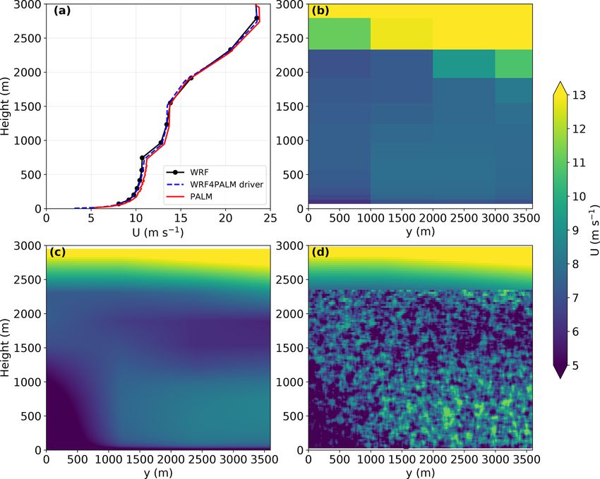
D. Lin et al.: WRF4PALM 2509
Figure 2. WRF domains configuration. Domains D01, D02, D03, and D04 with grid spacing of 27, 9, 3, and 1 km respectively (contains
imagery © Cartopy).
Table 3. PALM domain configuration for the case studies.
Directions Total Grid Grid
lengths points spacings
X 3600 m 360 10 m
Y 3600 m 360 10 m
Z∗ 2950 m 200 10 m
∗ Vertical grid spacing is trenched with a factor of 1.02
above z = 1200 m with max vertical grid spacing of 30 m.
tween 15:00 NZDT, 13 February and 15:00 NZDT, 14 Febru-
ary 2017, which have seen the sustained north-westerlies
over Christchurch. In Fig. 4, the time series of the WRF
modelling data have an hourly temporal interval while both
PALM modelling data and observational data are 1 min aver-
ages. Here both PALM and WRF winds are at 10 m in order
to compare with 10 m winds measured by the AWS. Both
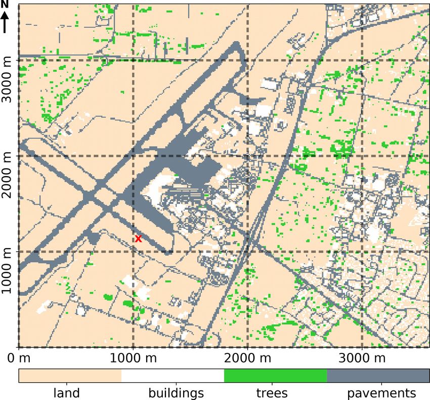
Figure 3. PALM modelling domain (3.6 km × 3.6 km) for the north- PALM and WRF modelled temperature data shown in Fig. 4
westerly case. Dotted black lines illustrate the grid size of the WRF are 2 m data to represent surface air temperatures. In order
model. Buildings are in white, trees are in green, pavements are in to show wind direction clearly and avoid overlapping data,
grey, and other types of surface are coloured in sand yellow. The red only 30 min wind direction PALM and observational data are
cross shows the AWS location. shown in Fig. 4. The time series of wind direction, wind
speed, and air temperature show good agreement between
the observational data and the modelled data. WRF overes-
pare the model data with the observational data and (2) avoid timated wind speed during the first 2 h shown in Fig. 4 and
possible artefacts produced by STG near the north and west underestimated wind speed between 05:00 and 08:00 NZDT,
lateral boundaries. A narrow zone of laminar flows near the 14 February. In addition, the air temperatures simulated by
lateral boundaries at inflow can appear in the simulation due WRF are approximately 2 ◦ C lower than the observed tem-
to the flow adjustment zone created by STG. As shown in perature during the entire 24 h period. Table 4 compares the
Fig. 4, this PALM simulation includes the 24 h period be- modelled surface temperature and wind speed with the ob-
https://doi.org/10.5194/gmd-14-2503-2021 Geosci. Model Dev., 14, 2503–2524, 2021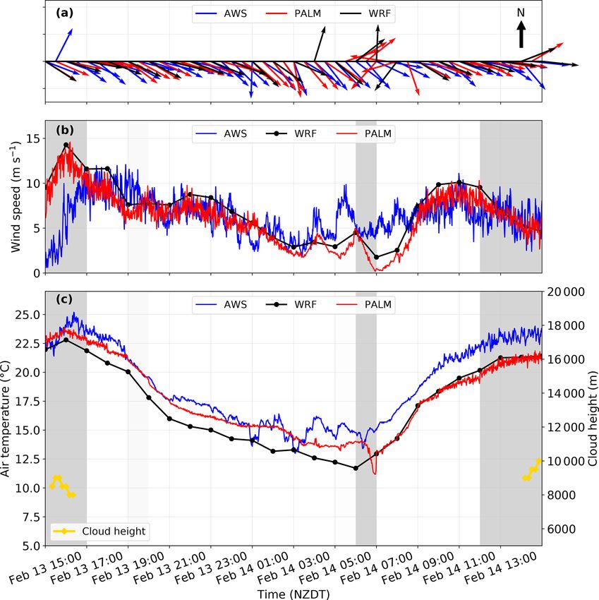
2510                                                                                                     D. Lin et al.: WRF4PALM

Figure 4. The time series of simulated (a) wind direction, (b) wind speed, and (c) air temperature for the north-westerly case between
15:00 NZDT, 13 February and 15:00 NZDT, 14 February 2017 compared with observations (labelled as AWS). In panel (c) the yellow line
indicates cloud height observed at the AWS. In panels (b) and (c), the shaded grey periods indicate when clouds are simulated in the WRF
model. Only 30 min PALM and observational data for wind direction are shown in (a) to avoid overlapping of arrows.

servational data. The root mean square error (RMSE),                  and Draxler, 2014 and Eq. 3 in Willmott et al., 2012 respec-
          v                                                           tively). Both RMSE and IOA are measures of the degree of
          u n                                                         model prediction error. The smaller the RMSE, the better the
          u1 X
RMSE = t           [Fi − Oi ]2 ,                              (4)     model fits to the observations. In terms of IOA, a value of 1
             n i=1
                                                                      indicates a perfect match while 0 indicates no agreement at
                                                                      all. The calculation is applied to the surface time series data
and index of agreement (IOA),
                                                                      shown in Fig. 4. Hourly averages of both PALM-simulated
                   Pn                                                 data and the observational data are taken in order to compare
                     i=1 |Fi − Oi |
IOA = 1 − Pn                              ,                   (5)     them with the WRF-simulated hourly data. Based on RMSE
              i=1 (|Fi − Ō| + |Oi − Ō|)                             (2.02 for temperature and 2.70 for wind speed) and IOA (0.72
are used for the comparison between modelled and ob-                  for temperature and 0.50 for wind speed) given in Table 4,
servational data, where Fi (i = 1, 2, . . ., n) indicates model       WRF results are satisfactory compared with other WRF stud-
estimates or predictions, Oi (i = 1, 2, . . ., n) indicates the       ies. For example, the best RMSE and IOA for wind speed in
pairwise-matched observations, and Ō is the mean value of            Indasi et al. (2017) are 2.30 and 0.66 respectively while they
observations (for details of the equations see Eq. 2 in Chai          also have simulations with RMSE of 4.21 and IOA of 0.43;

Geosci. Model Dev., 14, 2503–2524, 2021                                                 https://doi.org/10.5194/gmd-14-2503-2021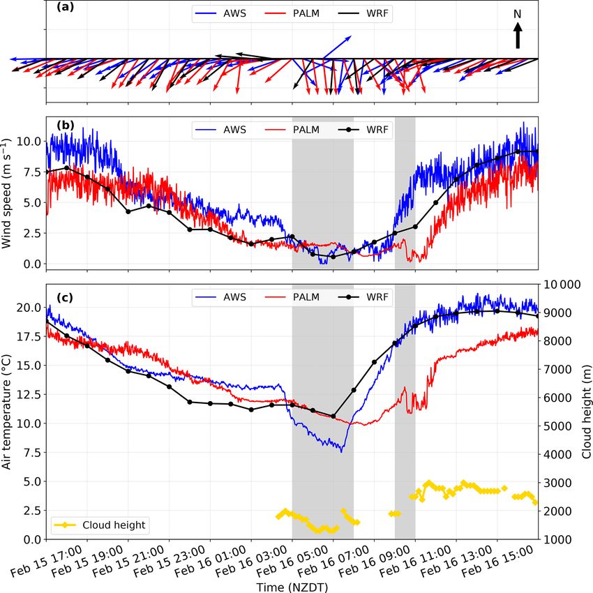
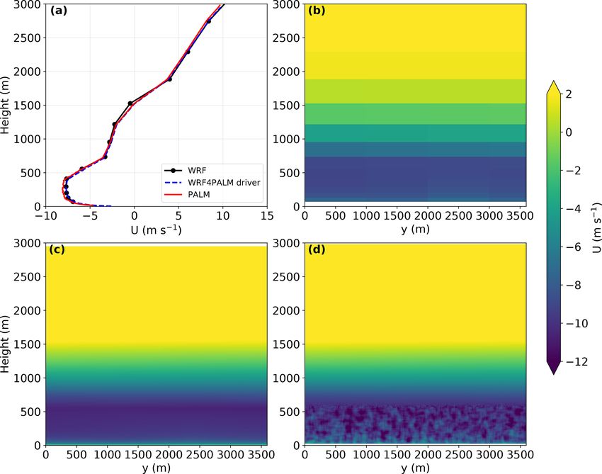
D. Lin et al.: WRF4PALM                                                                                                      2511

Figure 5. (a) Vertical profiles of the u component of winds in WRF, the WRF4PALM dynamic driver, and PALM at the initial time. The
profiles taken from WRF and PALM are both horizontally averaged. Vertical cross sections of the u component of winds taken from WRF
(nearest four grid cells) (b), the dynamic driver (c), and PALM (d) at 14:00 NZDT, 14 February 2017.

temperature simulated by WRF in Bhati and Mohan (2018)              vertical cross section at the left boundary). Profiles of other
has RMSE between 3.87 and 7.99 and IOA between 0.58                 parameters in the dynamic drivers are not shown here. The
and 0.81. Overall, PALM has smaller RMSE and higher IOA             WRF profiles are interpolated by WRF4PALM to the dy-
than WRF meaning that PALM has better performance than              namic driver, which is further used as an input for PALM
WRF regarding surface temperature and wind speed estima-            offline nesting. As shown in Fig. 5, profiles in the dynamic
tion in this case. The comparison between PALM and WRF              driver are generally identical to profiles in WRF meaning
also shows good agreement (IOA of 0.87 and 0.75 for surface         that WRF data are successfully interpolated and processed
temperature and wind speed respectively). The improvement           by WRF4PALM. Differences between profiles in PALM and
in observation-related RMSE and IOA by PALM is due to               WRF can be spotted (Fig. 5), which are due to the turbu-
the inclusion of surface geometries and the LES ability for         lence generated by the STG embedded in PALM. Figure 5
better resolving near-surface turbulence.                           shows that WRF4PALM successfully interpolates dynamics
   Throughout the 24 h period, the results in PALM align            from WRF and passes them to PALM through the dynamic
with those from WRF. The time series of surface winds and           driver. The boundary layer height is automatically calculated
temperatures in PALM shown in Fig. 4 are similar to those in        in PALM, which is 2300 m in Fig. 5d.
WRF, while PALM shows higher surface temperatures than                 The vertical profiles of the u component and v com-
WRF before 05:00 NZDT, 14 February 2017. To further vali-           ponent of winds and potential temperature (θ ) at 15:00
date the performance of WRF4PALM, comparisons between               and 21:00 NZDT on 13 February 2017 and at 03:00 and
WRF, the WRF4PALM dynamic driver, and PALM are car-                 09:00 NZDT on 14 February 2017 in PALM are almost iden-
ried out. Figure 5 compares the profiles of the u component         tical to vertical profiles in WRF as shown in Fig. 6, and the
of winds between WRF, the WRF4PALM dynamic driver,                  boundary layer heights in WRF and PALM are consistent
and PALM. The profiles include (1) the initial vertical pro-        over time. The maximum boundary layer height (MBLH) is
files and (2) left (west) boundary conditions (south–north          around 1.5–1.8 km in both WRF and PALM. The only ma-

https://doi.org/10.5194/gmd-14-2503-2021                                              Geosci. Model Dev., 14, 2503–2524, 2021
2512                                                                                                       D. Lin et al.: WRF4PALM

Figure 6. The north-westerly case. Vertical profiles of the u component of winds (a–d), v component of winds (e–h), and potential tempera-
ture (θ ) (i–l) taken from PALM and the WRF model at the times indicated in the figures (from left to right).

Geosci. Model Dev., 14, 2503–2524, 2021                                                  https://doi.org/10.5194/gmd-14-2503-2021
D. Lin et al.: WRF4PALM 2513
Table 4. Comparison of RMSE and IOA between the AWS observational data, the WRF modelling data, and the PALM modelling data at
surface. Here, wind indicates wind speed.
Counterparts Temperature RMSE Temperature IOA Wind RMSE Wind IOA
North-westerly case
AWS and WRF 2.02 0.72 2.70 0.50
AWS and PALM 1.44 0.81 2.42 0.56
WRF and PALM 0.91 0.87 1.54 0.75
North-easterly case
AWS and WRF 1.15 0.85 1.55 0.76
AWS and PALM 2.64 0.63 2.12 0.66
WRF and PALM 2.43 0.66 1.10 0.79
North-easterly case before 04:00 NZDT, 16 February 2017
AWS and WRF 1.13 0.79 1.60 0.63
AWS and PALM 0.99 0.74 1.76 0.56
WRF and PALM 1.17 0.74 1.00 0.77
North-easterly case after 04:00 NZDT, 16 February 2017
AWS and WRF 1.18 0.88 1.55 0.84
AWS and PALM 3.61 0.56 2.45 0.69
WRF and PALM 3.24 0.59 1.22 0.79
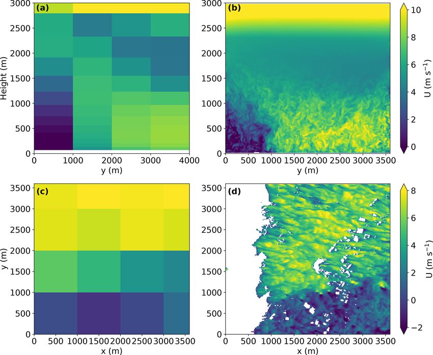
Figure 7. The north-westerly case. South–north vertical cross sections of the u component of winds taken from the WRF model (a) and
PALM (b) at 14:00 NZDT, 14 February 2017. Horizontal cross sections of the u component of winds taken from the lowest level in the WRF
model (c) and 5 m height in PALM (d) at 14:00 NZDT, 14 February 2017. White areas indicate terrain and buildings higher than 5 m above
the lowest level in the PALM simulation domain.
https://doi.org/10.5194/gmd-14-2503-2021 Geosci. Model Dev., 14, 2503–2524, 20212514 D. Lin et al.: WRF4PALM
layer dynamics developing their own unique state (Schalk-
wijk et al., 2015; Heinze et al., 2017). Hence, PALM fol-
lows most of the dynamics processed from WRF and this
could be further investigated by relaxing the update cycle
of PALM’s boundary conditions. In addition to the turbu-
lent time series of PALM shown in Fig. 4, Fig. 7 compares
the vertical and horizontal cross sections between WRF and
PALM. The WRF cross sections presented in Fig. 7 are the
nearest four WRF grid points (4 km × 4 km) processed to
the PALM domain (3.6 km × 3.6 km). The cross sections of
the two models show that PALM has strong agreement with
WRF. However, WRF is not able to resolve any surface ge-
ometries because it is a terrain following model and only sim-
Figure 8. Comparison of the range and distributions of hourly wind
speed anomalies between PALM and the observational data (la- ulates mesoscale characteristics of airflows. On the contrary,
belled as AWS) for the 24 h period of the north-westerly case. σ PALM’s Cartesian grid structure allows PALM to resolve
is the standard deviation of the anomaly data. all the terrain structure and urban canopy explicitly. White
patches and areas shown in Fig. 7d are buildings and ter-
rains that are higher than 5 m above the lowest level in the
PALM simulation domain. Microscale characteristics, such
as the local lift and drag forces as well as turbulence, are
only realised in PALM.
To demonstrate and further validate wind anomalies pro-
duced in the PALM simulation, Fig. 8 compares the modelled
wind speed anomalies in PALM to the anomalies observed by
the AWS. The wind anomalies are calculated by differencing
the instantaneous 1 min wind speed from the hourly averaged
wind speed for each hour during the 24 h simulation period.
As shown in Fig. 8, the modelled anomalies vary from ap-
proximately −4.2 to 3.5 m s−1 while the observed anomalies
vary from approximately −5.0 to 4.0 m s−1 . The standard de-
viation (σ ) of modelled data (2.662) is greater than the obser-
vational data (2.118). PALM created more positive anomalies
but with lower magnitude. The underestimation in the inten-
sity is likely to result from underpredictions in nighttime tur-
bulence generated by PALM incorporating the STG at inflow
or the biases produced in the model due to coarse grid spac-
ing (van Stratum and Stevens, 2015). The spatial resolution
Figure 9. As in Fig. 3, but for the north-easterly case. used in the PALM simulation is only 10 m, which may not
be sufficient to represent the nocturnal boundary layer prop-
erly. Despite the underestimation, PALM is able to reproduce
jor difference in the vertical profiles between the two mod- the wind trends and directions. The wind anomaly statistics
els can be spotted near the surface. This difference is due of WRF are not shown here because (1) the RANS mode of
to the impact of surface canopy because PALM is able to WRF only presents average properties of airflows and (2) the
explicitly resolve vegetation and building structures in the WRF output used here only contains hourly data, which can-
simulation. A spatial resolution of 10 m may not be suffi- not give any wind anomaly information at each hour during
cient to represent detailed structures of buildings, but such the simulation period.
resolution allows PALM to adequately represent most of the
surface geometries in the model domain. We believe the 4.3 North-easterly case
high similarity between PALM and WRF demonstrates suc-
cessful offline nesting using WRF4PALM. The lateral and In the late afternoons on 15 February 2017, easterly-north-
top boundaries of PALM are offline nested with WRF, and easterly flows were observed over Christchurch airport. Dur-
the mesoscale forcings from WRF are updated every hour. ing the early mornings on 16 February 2017, calm northerlies
Driving an LES model using hourly update cycles from a were recorded. Similar to the north-westerly case described
mesoscale model ensures mesoscale disturbances are rep- in Sect. 4.2, the PALM simulation domain (see Fig. 9) is
resented, but it may also hinder the microscale boundary designed to include the AWS and avoid artefacts near the
Geosci. Model Dev., 14, 2503–2524, 2021 https://doi.org/10.5194/gmd-14-2503-2021D. Lin et al.: WRF4PALM 2515 Figure 10. As in Fig. 4, but for the north-easterly case between 17:00 NZDT, 15 May 2017 and 17:00 NZDT, 16 May 2017. north and east lateral boundaries. Figure 10 shows the time and the observational data. The largest difference in surface series of wind direction, wind speed, air temperature, and temperature between PALM and both WRF and the obser- cloud height during the 24 h PALM simulation period from vational data is approximately 7 ◦ C. In terms of the RMSE 17:00 NZDT, 15 February 2017 to 17:00 NZDT, 16 Febru- and IOA for this case, shown in Table 4, PALM has worse ary 2017. Similar to the north-westerly case, profiles in WRF, scores than WRF, despite the fact that PALM still has ade- the WRF4PALM dynamic driver, and PALM are consistent quate agreement with WRF (IOA of 0.66 and 0.79 for sur- (Fig. 11). The vertical profiles shown in Fig. 12 and the ver- face temperature and wind speed respectively). The wind tical and horizontal cross sections shown in Fig. 13 all show anomaly analysis for the hourly averaged wind speed dur- good agreement between PALM and WRF. The MBLH for ing the entire 24 h simulation period is shown in Fig. 14. In this case is 900 m in both WRF and PALM. However, PALM this case, PALM only has an adequate performance in terms does not predict surface temperatures and winds as well as of modelling wind anomalies. Similar to the north-westerly in the north-westerly case described above. For the period case, anomalies simulated by PALM have more positive and after 07:00 NZDT, 16 February (see Fig. 10), PALM fol- smaller values. Due to the bias in the surface wind and tem- lows the increasing trends of surface temperature and wind perature, PALM also underestimated wind anomalies signif- speed in WRF, but the underestimation of surface temper- icantly. The modelled anomalies vary from approximately ature in PALM is significant. Wind speed in PALM is ap- −2.8 to 2.0 m s−1 , while the observational data show that proximately 2 m s−1 lower than both the WRF modelled data the anomalies have a range approximately −3.2 to 2.8 m s−1 . https://doi.org/10.5194/gmd-14-2503-2021 Geosci. Model Dev., 14, 2503–2524, 2021
2516                                                                                                         D. Lin et al.: WRF4PALM

Figure 11. As in Fig. 5, but for the north-easterly case. Panels (b), (c), and (d) are at 16:00 NZDT, 16 May 2017.

The standard deviation also shows underestimation in PALM                simulated radiation in PALM becomes unrealistic. Accord-
(2.238) compared with the observational data (2.953).                    ing to Table 4, the RMSE and IOA of surface temperature in
   There could be several reasons for the bias in PALM. Re-              PALM for clear sky periods (before 04:00 NZDT, 16 Febru-
gardless of different initialisation situations between the two          ary) are considerably better than the numbers for cloudy pe-
case studies, cloud cover is suspected to be one particular              riods (after 04:00 NZDT, 16 February). Another possible rea-
reason for errors in PALM. In both PALM simulations, the                 son for PALM’s poor performance could be the internal dy-
clear-sky radiation scheme is used. This radiation scheme                namics in PALM. As shown in Fig. 10, PALM simulated a
is the simplest scheme in the PALM modelling system and                  north-westerly airflow near the AWS site near 08:00 NZDT,
neglects all clouds. The observed cloud height and WRF-                  16 May 2017. The north-westerly air mass results in a more
modelled clouds are shown in Figs. 4 and 10. Here the vari-              convective surface and significant decrease in surface tem-
able cloud fraction is used to represent cloud cover in WRF.             perature in the west part of the PALM simulation domain
The grey shaded periods in Figs. 4 and 10 represent when the             (not shown). In this north-easterly case, the wind speed dur-
cloud fraction in WRF is greater than zero. Cloud fractions              ing the simulated period is generally low, which cannot offset
in WRF were averaged over the closest 10 grid cells over                 the convections in PALM domain. We believe the validation
the Christchurch airport. In the north-westerly case, most of            results of the PALM simulations with observations are not re-
the simulation period saw clear skies and only a small num-              lated to the technique of the offline nesting or WRF4PALM.
ber of high clouds (above approximately 7500 m) were ob-                 Rather, the dynamics, weather conditions, or PALM domain
served above the Christchurch airport and WRF generally                  configurations may be the possible factors. The PALM do-
correctly predicted cloud cover (see Fig. 4). In contrast, the           main location in this case is different from the north-easterly
period between 04:00 and 17:00 NZDT, 16 February saw sus-                case and the sensitivity of the domain grid spacing or domain
tained low level clouds (1000 to 3000 m) (see Fig. 10). WRF              size may also need to be evaluated. Further studies are re-
may have managed to have an adequate estimation of cloud                 quired to investigate why PALM underestimates surface tem-
cover during early mornings on 16 February and hence has a               perature and wind speed. However, this is beyond the scope
better performance than PALM in this north-easterly case.                of this study as here we only aim to validate WRF4PALM.
Because no clouds are simulated in clear-sky PALM, the                   Although PALM provides several radiation scheme options

Geosci. Model Dev., 14, 2503–2524, 2021                                                    https://doi.org/10.5194/gmd-14-2503-2021
D. Lin et al.: WRF4PALM                                                                                                  2517

Figure 12. As in Fig. 6, but for the north-easterly case between 17:00 NZDT, 15 May 2017 and 17:00 NZDT, 16 May 2017.

https://doi.org/10.5194/gmd-14-2503-2021                                               Geosci. Model Dev., 14, 2503–2524, 2021
2518                                                                                                    D. Lin et al.: WRF4PALM

Figure 13. As in Fig. 7, but at 16:00 NZDT, 16 May 2017 for the north-easterly case.

                                                                       validated by two case studies in Christchurch, New Zealand,
                                                                       in the summer season. WRF4PALM does not require users to
                                                                       pre-process any data manually, but users need to provide their
                                                                       WRF output and PALM domain configuration. WRF4PALM
                                                                       only encompasses mesoscale dynamics from WRF and does
                                                                       not require a static driver of PALM. In order to include sur-
                                                                       face heterogeneities, the PALM static driver is used in this
                                                                       study when it is necessary to realise microstructures in ur-
                                                                       ban environments and hence to achieve realistic and repre-
                                                                       sentative results in PALM simulations. In the case studies,
                                                                       WRF4PALM was applied to two weather events simulated
                                                                       by WRF for a north-westerly case and a north-easterly case
                                                                       in Christchurch, New Zealand. The case studies are designed
Figure 14. As in Fig. 8, but for the north-easterly case.
                                                                       to demonstrate the numerical stability of WRF4PALM rather
                                                                       than properly validate meteorology in the simulations. As
and has the bulk cloud module embedded, the detailed dy-               shown in the case studies, overall WRF4PALM is considered
namics in simulations may vary case by case and hence the              to have good stability and is able to process dynamics from
optimal simulation setup of PALM must be examined in fu-               WRF to PALM successfully. While PALM inherited most of
ture simulations.                                                      the characteristics from WRF through the WRF4PALM dy-
                                                                       namic driver, PALM’s ability to resolve turbulence structure
                                                                       is essential to realise and represent microscale dynamics in
5   Conclusions                                                        urban environments. A comparison of wind anomaly statis-
                                                                       tics also shows satisfactory agreement between PALM and
This study describes a utility WRF4PALM that is devel-                 the AWS observational data.
oped to generate mesoscale forcing from WRF output for the                For future use, the domain size, grid spacing, radiation
PALM model system 6.0. Results of the application are also             scheme, and all other model configurations of WRF and

Geosci. Model Dev., 14, 2503–2524, 2021                                                https://doi.org/10.5194/gmd-14-2503-2021
D. Lin et al.: WRF4PALM 2519 PALM need to be evaluated subject to the users’ own objec- tives and scope of research questions. In this study, the lat- eral and top boundary conditions in the WRF-PALM offline nesting are updated every 1 h meaning PALM is significantly impacted and constrained by WRF. The sensitivity to the re- laxation time and the STG configuration to develop initial turbulence need further assessment. WRF4PALM is distributed as a free and open-source tool. In the future, we aim to optimise WRF4PALM in terms of computation time and to further automate the process. As de- scribed in the PALM input data standard, the dynamic driver of PALM can also include boundary conditions of chemistry species, such as PM10 , NOx (NO2 , NO), and SO4 to simulate air pollution in urban environments. WRF4PALM has the po- tential to process chemistry data from WRF-Chem (the WRF model coupled with chemistry; Grell et al., 2005) to PALM using a similar interpolation technique as that described in Sect. 3.1. Although several tests and validations have been carried out for WRF4PALM, they may not be conclusive. To improve and extend the use of WRF4PALM, we welcome all users to optimise, modify, and contribute to the code. https://doi.org/10.5194/gmd-14-2503-2021 Geosci. Model Dev., 14, 2503–2524, 2021
2520                                                                                                 D. Lin et al.: WRF4PALM

Appendix A: WRF4PALM development                                1. Function to determine the nearest gird cells in WRF to
                                                                   be interpolated to the PALM Cartesian grid:
Based on ideas and techniques applied in WRF2PALM, the
                                                                     def nearest(array, number):
following changes have been made to develop WRF4PALM:                    '''
                                                                         find nearest index value and index in array.
                                                                         nearest(array, number)
  – add initial vertical profiles interpolated from WRF to               return(nearest_number, nearest_index)
                                                                         '''
    initialise PALM                                                      import numpy as np
                                                                         nearest_index = np.where(np.abs(array-number) ==
                                                                                         np.nanmin(np.abs(array-number)))
                                                                         nearest_index = int(nearest_index[0])
  – modify geostrophic wind calculation                                  nearest_number = array[nearest_index]
                                                                     return(nearest_number, nearest_index)

  – add create_cfg.py script to read user input to re-
    duce manual processing                                      2. Function to interpolate WRF data horizontally:
  – improve methods for PALM domain configuration,                   def interp_array_2d(data, out_x, out_y, method):
                                                                         '''
    which is almost identical to PALM input parameters                   2d matrix data, x number of points out_x, y number of points out_y,

                                                                        method 'linear' or 'nearest'
  – interpolation order is modified; horizontal interpolation           '''
                                                                        y = np.arange(0, data.shape[0], 1)
    is performed before vertical interpolation.                         x = np.arange(0, data.shape[1], 1)
                                                                        interpolating_function = RegularGridInterpolator((y, x), data,
                                                                                                                          method = method)

  – adjust physical heights calculated from WRF for verti-               yy, xx = np.meshgrid(np.linspace(x[0], x[-1], out_x),
                                                                                  np.linspace(y[0], y[-1], out_y))
    cal interpolation.                                                   data_res = interpolating_function((xx, yy))
                                                                     return (data_res)

  – adjust horizontal interpolation method for boundary
    conditions.                                                 3. Function to interpolate a 1-d array while calculating
                                                                   geostrophic winds:
  – adjust PALM domain height calculation for vertical in-
    terpolation and calculation of top boundary conditions           def interp_array_1d(data, out_x) :
                                                                         '''
                                                                         1d matrix data, x number of points out_x.
                                                                         Output a linear interpolated array
  – add staggered coordinates for wind field (u,v, and w)                '''
                                                                         x = np.arange(0, data.shape[0], 1)
    interpolation                                                        xvals = np.linspace(0, data.shape[0], out_x)
                                                                         data_res = np.interp(xvals, x, data)
                                                                     return (data_res)
  – add 3-D soil moisture and soil temperature profiles in-
    terpolated from WRF
  – allow PALM domain size smaller than one WRF grid
    cell size
  – allow users choose simulation period and update fre-
    quency based on WRF model outputs
  – add functions to create coordinate information for
    PALM self-nested domains
  – add surface NaN solver
  – add parameters and functions to enable vertically
    stretched grid spacing in the dynamic driver and sub-
    sequently PALM.

RAM (random access memory) usage is modified after the
aforementioned development and several other small tweaks
are made in WRF4PALM. WRF2PALM functions are either
removed or modified in WRF4PALM. The following Python
functions used in WRF4PALM are based on WRF2PALM:

Geosci. Model Dev., 14, 2503–2524, 2021                                        https://doi.org/10.5194/gmd-14-2503-2021
D. Lin et al.: WRF4PALM 2521
Appendix B: WRF4PALM step-by-step guide
A more detailed manual is available at https://github.com/
dongqi-DQ/WRF4PALM (last access: 23 April 2021).
B1 Step 1: specify the domain
Users first need to give the domain information in the
create_cfg.py script. The information includes
case_name_d01 = 'chch_10m_NW' # case name as you prefer, but should be
# consistent with the one used in dynamic script
centlat_d01 = -43.487 # latitude of domain centre
centlon_d01 = 172.537 # longitude of domain centre
dx_d01 = 10 # resolution in meters along x-axis
dy_d01 = 10 # resolution in meters along y-axis
dz_d01 = 10 # resolution in meters along z-axis
nx_d01 = 360 # number of grid points along x-axis
ny_d01 = 360 # number of grid points along y-axis
nz_d01 = 120 # number of grid points along z-axis
Run create_cfg.py to create a configura-
tion file containing the domain information for
create_dynamic.py.
B2 Step 2: process WRF for PALM
1. Specify case name, which should be the same as the one
specified in Step 1.
case_name = 'chch_10m_NW' # case name as specified in create_cfg.py
2. Specify the WRF output file to process.
wrf_file = 'wrfout_domain_yyyy-mm-dd'
3. Specify the start and end time stamp as well as the up-
date frequency of boundary conditions.
dt_start = datetime(2017, 2, 11, 0,) # start time in YYYY/MM/DD/HH format
dt_end = datetime(2017, 2, 12, 0,) # end time in YYYY/MM/DD/HH format
interval = 2 # specify update frequency
4. Specify the depth of soil layers.
dz_soil = np.array([0.01, 0.02, 0.04, 0.06, 0.14, 0.26, 0.54, 1.86])
# this is the default 8-layer setup in PALM
5. If stretched vertical grid spacing is desired, specify the
following parameters:
dz_stretch_factor = 1.02 # stretch factor for a vertically stretched grid
# set to 1 if no stretching is desired
dz_stretch_level = 1200 # Height level above which the grid cells
# are to be stretched vertically (in m)
dz_max = 30 # allowed maximum vertical grid spacing (in m)
6. Run create_dynamic.py and if successfully exe-
cuted, a dynamic driver file will be ready.
https://doi.org/10.5194/gmd-14-2503-2021 Geosci. Model Dev., 14, 2503–2524, 20212522 D. Lin et al.: WRF4PALM
Code availability. The WRF model system V4.0 and the WRF Pre- Financial support. Dongqi Lin and Laura E. Revell received sup-
processing System (WPS) V4.0 used in this study are free and port from the University of Canterbury and the Ministry of Busi-
open-source numerical atmospheric modelling systems (registration ness, Innovation and Employment project Particulate Matter Emis-
and download are available at https://www2.mmm.ucar.edu/wrf/ sions Maps for Cities (grant no. BSCIF1802). The contribution
users/download/get_source.html, last access: 23 April 2021). The of Basit Khan was supported by the MOSAIK and MOSAIK-
PALM model system 6.0 used in this study is freely available online 2 projects, which are funded by the German Federal Ministry
(http://palm-model.org, last access: 23 April 2021) under the GNU of Education and Research (BMBF) (grant nos. 01LP1601A and
General Public License v3. The exact PALM model source code (re- 01LP1911H), within the framework of Research for Sustainable
vision 4550) is available at https://doi.org/10.5281/zenodo.4713316 Development (FONA; http://www.fona.de, last access: 10 Au-
(Lin, 2020a) or https://palm.muk.uni-hannover.de/trac/browser? gust 2020). Marwan Katurji was supported by the Royal Soci-
rev=4550 (last access: 23 April 2021). WRF4PALM code is ety of New Zealand (contract no. RDF-UOC1701). Ricardo Faria
freely available at https://doi.org/10.5281/zenodo.4017005 (Lin, was financially supported by the Oceanic Observatory of Madeira
2020b) or https://github.com/dongqi-DQ/WRF4PALM (last access: Project (grant no. M1420-01-0145-FEDER-000001-Observatório
23 April 2021) distributed under GNU General Public License v3.0. Oceânico da Madeira-OOM).
Details of Python packages used in WRF4PALM are given on the
GitHub repository.
Review statement. This paper was edited by Paul Ullrich and re-
viewed by two anonymous referees.
Data availability. All PALM input files for the north-westerly case
described in Sect. 4.2, including the static driver, the WRF4PALM
dynamic driver, and its configuration file, are available in the Sup-
plement. New Zealand MetService maintains ownership of the raw
AWS data and is providing the data to the University of Canterbury
on the understanding that it is for the purposes of research. The raw References
AWS data may not be used for commercial gain. The raw AWS data
may not be made available to any third party, unless prior agreement Arakawa, A. and Lamb, V. R.: Computational design of the basic
has been obtained from MetService. dynamical processes of the UCLA general circulation model,
General circulation models of the atmosphere, 17, 173–265,
1977.
Baldauf, M., Stephan, K., Klink, S., Schraff, C., Seifert, A., Först-
Supplement. The supplement related to this article is available on-
ner, J., Reinhardt, T., and Lenz, C.: The new very short range
line at: https://doi.org/10.5194/gmd-14-2503-2021-supplement.
forecast model COSMO-LMK for the convection-resolving
scale, WGNE Blue Book, Research activities in atmospheric and
oceanic modelling, CAS/JSC Working Group on Numerical Ex-
Author contributions. RF provided the WRF2PALM code. BK and perimentation, Report No. 37, WMO, Geneva, Switzerland, 1–2,
DL contributed to the initial development of WRF4PALM. DL 2007.
contributed to major WRF4PALM development and distribution. Bengtsson, L., Andrae, U., Aspelien, T., Batrak, Y., Calvo, J., de
LB helped DL with setting up WRF simulation. DL carried out Rooy, W., Gleeson, E., Hansen-Sass, B., Homleid, M., Hortal,
the WRF and PALM simulations and analysed the data. MK and M., Ivarsson, K., Lenderink, G., Niemelä, S., Nielsen, K. P.,
LER supervised DL in performing the case studies. DL wrote the Onvlee, J., Rontu, L., Samuelsson, P., Muñoz, D. S., Subias,
manuscript with contributions from BK, MK, and LER. BK, MK, A., Tijm, S., Toll, V., Yang, X., and Køltzow, M. Ø.: The
and LER reviewed the manuscript. HARMONIE–AROME model configuration in the ALADIN–
HIRLAM NWP system, Mon. Weather Rev., 145, 1919–1935,
https://doi.org/10.1175/MWR-D-16-0417.1, 2017.
Competing interests. The authors declare that they have no conflict Bergot, T., Escobar, J., and Masson, V.: Effect of small-scale sur-
of interest. face heterogeneities and buildings on radiation fog: Large-eddy
simulation study at Paris–Charles de Gaulle airport, Q. J. Roy.
Meteor. Soc., 141, 285–298, 2015.
Acknowledgements. We would like to thank Iman Soltanzadeh and Bhati, S. and Mohan, M.: WRF-urban canopy model evaluation for
Neal Osborne from New Zealand MetService for providing au- the assessment of heat island and thermal comfort over an urban
tomatic weather observations in Christchurch, New Zealand. We airshed in India under varying land use/land cover conditions,
thank Rui Caldeira from the Oceanic Observatory of Madeira for in- Geosci. Lett., 5, 27, https://doi.org/10.1186/s40562-018-0126-7,
ternal review of the original manuscript. Dongqi Lin acknowledges 2018.
Jiawei Zhang at the University of Canterbury for his help regard- Chai, T. and Draxler, R. R.: Root mean square error (RMSE)
ing technical issues related to PALM simulations. All PALM sim- or mean absolute error (MAE)? – Arguments against avoid-
ulations presented in this study were performed on New Zealand ing RMSE in the literature, Geosci. Model Dev., 7, 1247–1250,
eScience Infrastructure (NeSI) high-performance computing facili- https://doi.org/10.5194/gmd-7-1247-2014, 2014.
ties. WRF simulations were performed on the University of Canter- Envirionment Canterbury Regional Council: Christchurch and Ash-
bury high-performance computing cluster. ley River, Canterbury, New Zealand 2018, Open Topography,
https://doi.org/10.5069/G91J97WQ, 2020.
Geosci. Model Dev., 14, 2503–2524, 2021 https://doi.org/10.5194/gmd-14-2503-2021You can also read