Physical Initialisation of Precipitation in a Mesoscale Numerical Weather Forecast Model
←
→
Page content transcription
If your browser does not render page correctly, please read the page content below
Physical Initialisation of
Precipitation in a Mesoscale
Numerical Weather Forecast
           Model

                     Dissertation
                         zur
     Erlangung des Doktorgrades (Dr. rer. nat.)
                         der
   Mathematisch-Naturwissenschaftlichen Fakultät
                         der
   Rheinischen Friedrich-Wilhelms-Universität Bonn

                    vorgelegt von
                   Marco Milan
                         aus
                   S. Pietro in Gu

                     Bonn, 2009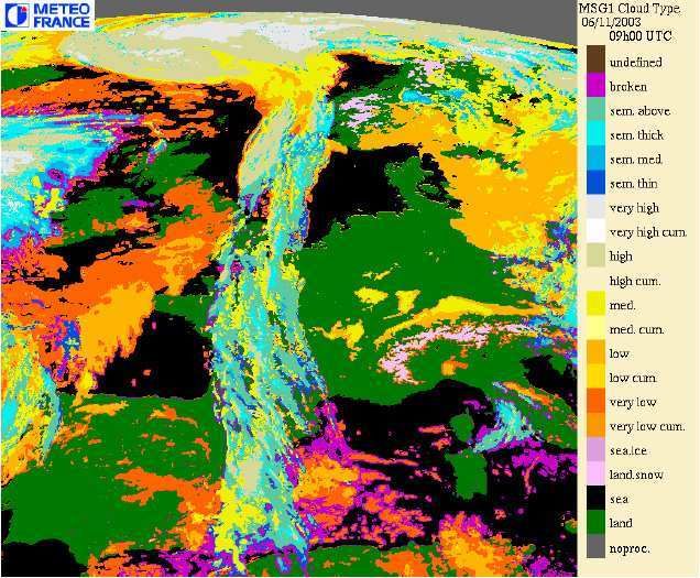
Angefertigt mit Genehmigung der Mathematisch-Naturwissenschaftlichen
Fakultät der Rheinischen Friedrich-Wilhelms-Universität Bonn

1. Referent: Prof. Dr. Clemens Simmer
2. Referent: Prof. Dr. Andreas Hense

Tag der Promotion: 02/02/2010
Erscheinungsjahr: 2010
Abstract

Short term quantitative precipitation forecast (QPF) is an important task
for numerical weather prediction (NWP) models, particularly in summer.
The increase of model resolution requires the understanding of the initiation
and evolution of convection. Initialisation schemes based on radar derived
precipitation fields can reduce the model forecast error in convective cases.
Any improvement of QPF denotes a correct forecast of the dynamics and the
moisture content of the atmosphere, thus upgrading QPF generically improves
NWP forecast.
The method, which we call Physical initialisation Bonn (PIB), uses as the most
important input the precipitation estimation from the German weather service
(DWD) radar network and assimilates the data into the operational non-
hydrostatic COSMO model. During the assimilation window, PIB converts
the input data (radar precipitation and cloud top height from satellite data)
into prognostic COSMO variables, which are relevant for the development of
rain events. PIB directly adjusts vertical wind, humidity, cloud water, and
cloud ice in order to force the model state towards the measurements. The
most distinctive feature of the algorithm is the adjustment of the vertical wind
profile in the framework of a simple precipitation generation scheme.
In a first study we performed an identical twin experiment with three
convective cases. The consistency of PIB with the physics of the NWP
model is proved using qualitative comparisons and quantitative evaluations
(e.g. objective skill scores).
The performance of PIB, using real data, is investigated by applying the
scheme to the whole month of August 2007, with three simulations every day, at
00, 08 and 16 UTC. Every simulation consists of two hours of data assimilation
followed by seven hours of free forecast. The comparison with the Control run
and with Latent heat nudging, the operational radar data assimilation scheme
from the DWD, is also made. PIB succeeds in improving QPF for up to six
hours. Its results are comparable to the forecast by LHN. The sensitive of PIB
to different assimilation windows is tested. An assimilation window of only
15 minutes is enough to provide the trigger for convection and to enhance the
forecast quality. Thus PIB is much more time efficient than LHN and need
much less observation values.
Contents

1 Introduction                                                                                                  1
  1.1 Motivation . . . . . . . . . . . . . .   .   .   .   .   .   .   .   .   .   .   .   .   .   .   .   .    1
  1.2 Assimilation techniques . . . . . . .    .   .   .   .   .   .   .   .   .   .   .   .   .   .   .   .    5
       1.2.1 Non variational approaches .      .   .   .   .   .   .   .   .   .   .   .   .   .   .   .   .    6
       1.2.2 Variational approaches . . .      .   .   .   .   .   .   .   .   .   .   .   .   .   .   .   .    9
  1.3 Data assimilation strategies . . . .     .   .   .   .   .   .   .   .   .   .   .   .   .   .   .   .   11

2 Model and data                                                                                               13
  2.1 COSMO model . . . . . . . . . . . . . . . . . . . . .                            .   .   .   .   .   .   13
      2.1.1 Data Assimilation in COSMO . . . . . . . . .                               .   .   .   .   .   .   16
      2.1.2 Initial and boundary conditions . . . . . . . .                            .   .   .   .   .   .   17
      2.1.3 Forecast and assimilation cycle . . . . . . . .                            .   .   .   .   .   .   18
      2.1.4 Grid scale precipitation . . . . . . . . . . . . .                         .   .   .   .   .   .   18
  2.2 Radar data . . . . . . . . . . . . . . . . . . . . . . .                         .   .   .   .   .   .   19
      2.2.1 RY product . . . . . . . . . . . . . . . . . . .                           .   .   .   .   .   .   19
      2.2.2 Typical errors in radar precipitation estimates                            .   .   .   .   .   .   20
      2.2.3 The composite . . . . . . . . . . . . . . . . .                            .   .   .   .   .   .   23
  2.3 Satellite data . . . . . . . . . . . . . . . . . . . . . .                       .   .   .   .   .   .   23
      2.3.1 Cloud top temperature and height . . . . . . .                             .   .   .   .   .   .   24
      2.3.2 Cloud type . . . . . . . . . . . . . . . . . . .                           .   .   .   .   .   .   24

3 The PIB algorithm                                                                                            27
  3.1 Analysed precipitation . . . . . . . . . . .             .   .   .   .   .   .   .   .   .   .   .   .   28
  3.2 Precipitation scheme . . . . . . . . . . . .             .   .   .   .   .   .   .   .   .   .   .   .   29
      3.2.1 Conversion efficiency determination                .   .   .   .   .   .   .   .   .   .   .   .   34
  3.3 Cloud Analysis . . . . . . . . . . . . . . .             .   .   .   .   .   .   .   .   .   .   .   .   35

                                       i
ii CONTENTS
3.3.1 Cloud base height . . . . . . . . . . . . . . . . . . . . . . 35
3.3.2 Cloud top height . . . . . . . . . . . . . . . . . . . . . . 37
3.3.3 Corrections . . . . . . . . . . . . . . . . . . . . . . . . . 39
3.4 Modification of model profiles . . . . . . . . . . . . . . . . . . . 40
3.4.1 Forcing of precipitation . . . . . . . . . . . . . . . . . . . 40
3.4.2 Suppression of precipitation . . . . . . . . . . . . . . . . 42
4 Identical twin 45
4.1 Case studies . . . . . . . . . . . . . . . . . . . . . . . . . . . . . 48
4.1.1 Case 1 : June 29, 2005 . . . . . . . . . . . . . . . . . . . 48
4.1.2 Case 2 : August 19, 2005 . . . . . . . . . . . . . . . . . . 49
4.1.3 Case 3 : June 28, 2006 . . . . . . . . . . . . . . . . . . . 50
4.2 Precipitation and CAPE field . . . . . . . . . . . . . . . . . . . 51
4.3 Cloud base in the convective regions . . . . . . . . . . . . . . . 61
4.4 Mass flux divergence . . . . . . . . . . . . . . . . . . . . . . . . 65
4.5 PIB without vertical wind or without humidity assimilation . . 71
4.5.1 Precipitation . . . . . . . . . . . . . . . . . . . . . . . . 71
4.5.2 Vertical wind . . . . . . . . . . . . . . . . . . . . . . . . 74
4.6 Summary of the Identical twin experiment . . . . . . . . . . . . 76
5 Real data assimilation 79
5.1 Evaluation of the free forecast . . . . . . . . . . . . . . . . . . . 80
5.1.1 Precipitation PDF and PDF of RADAR/MODEL . . . . 80
5.1.2 Relative precipitation . . . . . . . . . . . . . . . . . . . . 83
5.1.3 Objective skill scores . . . . . . . . . . . . . . . . . . . . 88
5.2 Duration of the assimilation window . . . . . . . . . . . . . . . 90
5.3 Summary of the real data experiment . . . . . . . . . . . . . . . 96
6 Conclusions and future research 97
6.1 Synthesis of the results . . . . . . . . . . . . . . . . . . . . . . . 97
6.2 Future work . . . . . . . . . . . . . . . . . . . . . . . . . . . . . 100
A Forecast verification methods 101
A.1 Objective skill scores . . . . . . . . . . . . . . . . . . . . . . . . 102
A.2 Root mean square difference . . . . . . . . . . . . . . . . . . . . 105CONTENTS iii
B Differences par. seq. 107
B.1 The Newtonian approximation method . . . . . . . . . . . . . . 107
B.1.1 First Newton’s method . . . . . . . . . . . . . . . . . . . 108
B.1.2 Newton’s method . . . . . . . . . . . . . . . . . . . . . . 108
B.2 Newton’s method in COSMO . . . . . . . . . . . . . . . . . . . 109
C CAPE 111
D Additional figures of chapter 4 113
Bibliography 117iv CONTENTS
Chapter 1

Introduction

Clouds and precipitations are essential components of the earth’s water and
energy cycle; they are important meteorological parameters of our habitat and
influence life in various ways.
The accurate forecast of precipitation events, particularly for heavy
precipitation, is of capital interest for the economy. For many applications
a Quantitative Precipitation Forecast (QPF) is essential. In agriculture,
precipitation can have different effects, sometimes positive, sometimes negative
depending also on the quantity. In hydrology, precipitation is the input of a
range of simulation models, e. g. for runoff prediction, flashflood warnings,
and water use and quality management. By improving QPF severe weather
warnings can be issued more precisely, and reduce flood damages and save
lives.
The goal of this work is the improvement of QPF, especially for convective
events in the midlatitudes. We are particularly interested in improving the
short time range forecast, up to about 9 hours.

1.1     Motivation
A Numerical Weather Prediction (NWP) model integrates the governing
equations of hydrodynamics using numerical methods subject to specified
initial conditions. Numerical approximations are fundamental to almost all
dynamical weather prediction schemes since the complexity and nonlinearity
of the hydrodynamic equations do not allow exact solutions of the continuous
equations. For this reason meteorology was one of the very first fields of
physical science that had the opportunity and necessity to exploit high speed
computers for the solution of multi-dimensional time-dependent non-linear
problems (Mesinger and Arakawa, 1976 [71]).

                                       1
2 CHAPTER 1. INTRODUCTION In the early NWP experiments (the first unsuccessful one was from Richardson in 1922 [81]) the need for an automatic “objective” analysis became quickly apparent (Charney, 1951 [17]). The analysis is a procedure to estimate the atmospheric dependent variables on a regular two- or three-dimensional grid using the data available from irregularly spaced observation networks (Daley, 1991, [26]). The determination of the initial condition for a NWP model and the subsequent assimilation of new observation data in the model run are fundamental for the quality of the forecast. The right determination of the model prognostic variables for the analysis provides the forecast model with the starting point, from which we can make the prognosis. The most difficult weather element to predict correctly is rainfall ( Ebert et al. 2003, [34]) because it is not a continuous field in space and time, like wind and temperature for instance; it is rather a collection of solid or liquid particles developed within weather systems with a typical life time between an hour to few days. Furthermore its formation and evolution is highly complex and nonlinear and occurs on scales that are several orders of magnitude smaller than the size of a numerical grid box (in our case the grid box has a dimension of 2.8km × 2.8km, while rain develops in spatial scales smaller than 1cm). Parameterisation schemes are therefore used to treat subgrid scale processes such as precipitation, but these had to be simplified for reasons of computational efficiency or the lack of knowledge about the true characteristics of those processes. We have to remark that normally the QPF skill also varies seasonally (Uccellini et al. 1999, [93], Weckwert et al. 2004 [96]) with the summer marked by lower forecast skill (we can clearly see this in terms of Threat Score in Fig. 1.1, for the definition of threat score see appendix A). The problem of warm season QPF is the high unpredictability of the convective events (Lorenz, 1969 [68]). These events are particularly challenging to predict because of their small spatial scale, short lifetime and non-linear, chaotic behaviour. In the current NWP models convection is parameterized. It is believed that an improved representation of convection in forecast models is a necessary path through which major advances in QPF will be realized. One necessary condition for a prediction of convective rainfall is a good forecast of where and when convection will initially develop; moreover the knowledge of the atmospheric state before the development of convection is crucial in order to initialise the NWP model. Currently the prediction and understanding of convection initiation processes, as well as the subsequent intensity, areal coverage and distribution of convective rainfall, are largely impeded by inaccurate and incomplete water vapour measurements (National Research Council, 1998 [22]).
1.1. MOTIVATION                                                                3

Figure 1.1: Monthly threat scores for quantitative precipitation forecasts for
the period form Jan 1991 to Dec 1999. Threat scores are plotted for the
NGM (Nested Grid Model, green histogram) and for the HPC (Hydrometeorol.
Prediction Center) forecaster predictions (red line) for the 24h period., picture
from Wecwert at all., 2004 [96]
4                                             CHAPTER 1. INTRODUCTION

The improvement of precipitation forecasts depends strongly on the coupling
of humidity and wind fields (Zou and Xiao, 2000 [104]). An error in the
initial state can amplify through the modelling process and result in drastic
under or overpredictions of precipitation (Park, 1999 [77]). A model-consistent
assimilation of precipitation and the corresponding fields of humidity can
reduce the lack in the hydrological variables results in the so called spin-up
(spin-down) problem (Krishnamurti, 1993 [57]), i.e. a hydrological imbalance
between precipitation and evaporation (e.g. Fig. 1.2). This improvement
is especially beneficial for nowcasting and short-range forecasting, with an
improvement of the forecast for surface pressure and dynamics.
Chang and Holt (1994 [16]) used a theoretical experiment and showed that,
for winter cases, the improvements in precipitation forecast due to data
assimilation are still noticeable after 30 hours of forecast.
Another study (Anderson et al., 2000 [4]) has investigated the impact
of observations on meso-scale model forecasts of three-hourly rainfall
accumulations. They assimilated three-dimensional humidity fields from the
Moisture Observation Processing System (MOPS). The main output from
MOPS consists of a three-dimensional analysis of cloud fraction. This is
converted into a set of relative humidity soundings at each model grid point,
which are then assimilated in the same way as radiosondes (Wright, 1993 [99]).
The MOPS leads to a significant increase in the forecasts quality. This is a
proof of the importance of humidity assimilation in NWP (see also Macpherson
et al., 1996 [69] ).
The reason for the model forecast improvement due to the humidity
assimilation is that QPF is directly linked to the model’s water cycle. The
spin-up problem is due to the fact that NWP model simulations are typically
initialised in so-called dry state, leaving the state variables for condensed water
at zero. Usually several hours of simulated weather evolution will pass until
the hydrological cycle is established in such a quasi-equilibrium.
Another parameter that influences the skill of QPF is orography; its forcing is
generally badly reproduced by the model dynamics, the precipitation pattern
(Gollvik, 1999 [40]) are especially poor for convective events in these areas. In
our work, therefore, we started with simulations in an area where orography
is not such an important factor (northern Germany) and then we applied the
model using a larger domain covering Germany as a whole including the alps.
In this way we tested the improvement of our scheme in both situations: with
and without complex orography.
We have implemented an assimilation technique that tries to improve the
forecast in terms of location, structure and movement within the area of
activity. The special aim is to improve nowcasting (about two hours) and
1.2. ASSIMILATION TECHNIQUES                                                  5

short range forecasts (less then 24 hours). Specifically we restricted our
self to predictions of only 9 hours, because the life cycle of the assimilated
synoptic situation in the studied area was shorter than that. The benefit of
data assimilation in high resolution models (in this case 2.8 km) for longer
periods decreases because of the increase of unpredictability with the spatial
resolution in the NWP models (Germann and Zawadzki, 2002 [38]) and the
increasing influence of the boundaries.
For model output evaluation a comparison with radar observations is
performed, by Objective Skill Scores (OBSS, defined in appendix A) and other
statistical quantities.

1.2     Assimilation techniques
In order to perform a numerical weather forecast, it is necessary to have
not only an appropriate numerical model but also a description of the
corresponding initial conditions as accurate as possible (Talagrand, 1997 [90]).
In the early NWP model experiments (Richardson, 1922 [81], and Charney et
al., 1950 [18]) the initial conditions were derived from an interpolation of the
available observations to the grid, and these fields were manually digitized.
It becomes immediately clear that a production of an automatic objective
analysis was necessary also in order to economize time.
The available observations, however, do not provide the temporally
synchronous and the spatially homogeneous description of the atmosphere,
that is required by a numerical model. Moreover many observations are in
quantities that are not prognostic model variables (for example in our case
reflectivity from radar data has to be converted into precipitation rate). In
this sense, assimilation is the process by which observations are combined
together with a numerical model in order to produce, as accurate as possible,
a description of the state of the atmosphere in terms of model variables.
The description of that atmospheric state is called analysis. It tries to
reproduce the true state using observations.
In case the model state is overdetermined by the observations, the analysis
reduces to an interpolation problem (Bouttier and Cortier, 1999 [13]). In
most cases the analysis problem is under-determined because data is sparse
especially in ocean regions. Moreover, in these regions most of the data are
only indirectly related to the model variables (e. g. satellite data).
In order to make analysis a well-posed problem it is necessary to rely on some
background (or first guess) information in the form of an a priori estimate of
the model state. The background could be a climatological state or, in the
6                                                   CHAPTER 1. INTRODUCTION

recent concepts, a previous forecast. Using the background state and the new
observations a new state for the atmosphere is given from the assimilation
techniques. This state will be propagated using the NWP model. For more
detailed information about data assimilation concepts the reader is referred
to Daley, 1991 [26] or Kalnay, 2003 [53] or Bouttier and Courtier, 1999 [13].
In this section we will describe briefly only some methods, in order to have a
general idea about data assimilation.
We can subdivide the assimilation techniques basically in two categories:
variational and non-variational.

1.2.1     Non variational approaches
Successive corrections method

We take a dependent variable f (~r) (Daley, 1991 [26] ), where ~r defines the
spatial location. The ~ri is the ith analysis gridpoint and ~rk the kth observing
location. The letter O stands for observation, B for background and A for the
analysis, the error is ǫ. For example the background error at an analysis grid
point i is ǫB (~ri ).
If we consider a single observation ~rk we can estimate the analysis increment
at the analysis gridpoint i :

                     fA (~ri ) − fB (~ri ) = Wik [fO (~rk ) − fB (~rk )]        (1.1)
where [fO (~rk ) − fB (~rk )] is the observation increment and Wik depends on
the expected background and observation error variance. The observation
increment is related to a weight depending on the distance w(~rk − ~ri ) (in
the original system from Cressman, 1959 [24] the weight depends only on the
distance). For such a system it si problematic to define the weight function,
Wik .
Assume that the background error is homogeneous and the observation errors
are spatially uncorrelated. Then equation 1.1 at the first iteration step can be
written as

                          fA1 (~ri ) = fB (~ri ) + WiT [f~O − f~B ]             (1.2)

where f~O and f~B are column vectors of lenght Ki (the number of observations
available in the range of influence) and Wi is a column vector of length Ki of
weights.
At this point an iteration process is applied. The second step uses the fA1 as
background and we have fA2 (~ri ) = fA1 (~ri ) + WiT [f~O − f~B ]. Then we iterate the
1.2.1.0 Optimal interpolation 7
process for n times, until convergence.
Optimal interpolation
Optimal interpolation, also called statistical interpolation (Daley, 1991 [26]),
is a minimum variance method. The basic form is the same as the successive
correction method. If we take K observation points for the analysis influencing
the ith point we get:
X
K
fA (~ri ) = fB (~ri ) + Wik [fO (~rk ) − fB (~rk )] (1.3)
k=1
or, with a more common notation (generally used in the variational approach):
P
Ai = Bi + K k=1 Wik [Ok − Bk ]. The optimal interpolation uses a minimum
variance estimation procedure for the definition of the weights Wik . This
assimilation scheme tries to minimize the expected analysis error variance as a
function of the weights. The expected analysis error variance is < (Ai −Ti )2 >,
where Ti is the true value at the point i. In this assimilation system both the
background field and the observations are assumed to be unbiased.
Latent heat nudging
The Latent Heat Nudging (LHN) scheme is based on the work of Manobianco et
al. (1994, [70]) and on the successive application from Jones and Macpherson
(1997, [50]). The principal idea is to correct the model’s latent heating at each
time step by an amount calculated from observed and modelled precipitation.
They assumed that the vertically integrated latent heating is proportional
to the surface rain rate (Leuenberger D., 2005 [65] ). Practically this
scheme nudges (Anthes, 1974 [5] and Hoke and Anthes, 1976 [45]) the model
temperature profile to the estimated temperature profile (using a saturation
adjustment technique).
The extra heating is a source term in the prognostic model temperature
equation and that changes the buoyancy and by ascent the precipitation. For
a description of LHN and its use in recent years see Leuenberger, 2005 [65],
Leuenberger and Rossa, 2004 [66] and Klink and Stephan, 2004 [54].
The Physical Initialisation scheme
The idea of using precipitation data in NWP models was in the first
experiments applied in the tropics (Krishnamurti et al. 1984 [58]). The use
of an assimilation technique in such an area was necessary because of the8 CHAPTER 1. INTRODUCTION
sparse presence of the classical data (for example radiosonde and synoptic
station), especially over oceanic areas. In the tropics the sparsity of data also
results in large errors in the divergent wind which in turn usually compounds
the humidity errors through moisture convergence, resulting in a erroneous
specification of the diabatic forcing (Krishnamurti et al., 1991 [59]). The
spin up problem (described in Fig. 1.2) is inherent to any NWP models
(Krishnamurti et al., 1988 [56]). The work of Krishnamurti tries to reduce
it by assimilating the precipitation fields (a review of this work can be found
in Krishnamurt et al., 1996, [55]).
Figure 1.2: Globally averaged value of evaporation and precipitation (units
mm · day −1 ) plotted as a function of forecast period. Krishnamurti et al. 1988,
[56]
Krishnamurti used a nudging scheme (or Newtonian relaxation ) involving
linear forcing to lead the evolution of variables towards certain predetermined
space-time estimates. The general form of the equation for these processes is:
∂A(x, y, t)
= F (A, x, y, t) + N(A, t) · (A0 (x, y, t) − A(x, y.t)) (1.4)
∂t
Where A is the predicted value of the variable at a time level during time
integration and A0 is the predetermined true estimate of the variable at that
time (analysis); F (A, x, y, t) is the time rate of change for the variable A due
to various dynamical and physical processes in the numerical model; N(A, t)
is the relaxation coefficient, the value that determines the degree with which
the variable is forced towards its analysed value A0 .
When the model predicted value A is equal to the analysed value the Newtonian
term (the second on the right side in the eq. 1.4) does not operate. The value1.2.2 Variational approaches 9
of the relaxation coefficient can be selected experimentally; a large relaxation
coefficient will force the variable too strongly, resulting in dynamic imbalance,
while a too weak relaxation coefficient is not efficient.
The Krishnamurti scheme uses a reverse Kuo algorithm for the improvement
of the humidity analysis. In the Kuo algorithm the moistening and heating
by the cumulus cloud are made using the temperature difference between the
cloud and the undisturbed environment and the large scale convergence of
moisture as indicators (Kuo, 1974 [62]). Therefore Krishnamurti et al. tried to
find an analysis of the humidity field consistent with an imposed precipitation
field and a cumulus parameterisation algorithm. For each time step a reverse
cumulus parameterisation algorithm provides a modified humidity field over
the convective areas each time step. A forward prediction of the humidity
variable with a direct Kuo algorithm nearly reproduces the imposed rain.
In the reverse Kuo scheme the specific humidity is calculated using the relation:
1 R pB Z pB
R g pT
qdp 1 ∂q
qm (p) = 1 R pB ∂q q(p) + 1 R pB × [1 − R/(− ω dp)] (1.5)
− g pT ω ∂p dp g pT
dp g pT ∂p
where q(p) and qm (p) are the original and modified values of specific humidity
at pressure level p, ω is the vertical velocity and pB and pT denote the bottom
and top pressure of the cumulus column, respectively. The modification is
applied only in the precipitation regions, with:
Z pB
1 ∂q
− ω dp > 0 (1.6)
g pT ∂p
and with the restriction qm (p) ≤ qs . In other words the modified specific
humidity has as upper limit the saturation value. This scheme was based on
observations from satellites and raingauges.
Krishnamurti’s scheme in the rain-free areas has a humidity adjustment based
on the two estimates (model and satellite) of the outgoing longwave radiation
above the planetary boundary layer (PBL). The scheme used a measure of the
advective-radiative imbalance and tries to minimize it using a modification of
q.
1.2.2 Variational approaches
Variational approaches consider the atmospheric state system as a whole and
do not deal explicitly with the individual components of the system. It involves
the determination of stationary points (Daley,1991 [26]) of integral expressions10 CHAPTER 1. INTRODUCTION
known as functionals1 . A stationary point is a point (in the domain of the
functional) where the rate of change of the functional in every possible direction
from that point is zero.
One disadvantage of this approach, as for Optimal Interpolation and all
versions of the Kalman filter, is the assumption of Gaussian error distributions.
3D-VAR
We can write the optimal interpolation scheme (for the notation see table 1.1)
as xa = xb + K[y − H[xb ].
Table 1.1: Notation used in this section with the dimensions of the matrixes
variable dim variable dim
xt true model state n xb background model state n
xa analysis model state n y vector of observations p
cov. matrix of the
H observation operator n → p B n×n
background error
cov. matrix of the cov. matrix of the
R p×p A n×n
observation error analyse error
K weight matrix n×n
The three dimensional variational assimilation principle tries to avoid the
computation of the weight matrix K completely by looking for the analysis
as an approximate solution of the equivalent minimization problem defined by
a cost function J, which could be seen as a measurement of the distance of the
estimate state from the observations.
J(x) = (x − xb )T B−1 (x − xb ) + (y − H[x])T R−1 (y − H[x]) (1.7)
The problem is now to find the minimum of J using the gradient ∇J(x);
usually a descent algorithm is used.
In 3D-Var the B matrix must be defined, i.e. the background error covariance
for all pairs of model variables.
4D-VAR
4D-Var is a generalization of 3D-Var for observations that are distributed in
time. We must include a forecast model operator M and an index i for the
model time; M0→i is the forecast model operator from the initial time to i.
1
functional: the principal meaning is a function whose domain is a set of functions1.3. DATA ASSIMILATION STRATEGIES 11
The cost function is now defined as:
X
n
J(x) = (x − xb )T B−1 (x − xb ) + (yi − Hi [xi ])T R−1
i (yi − Hi [xi ]) (1.8)
i
In this equation we assume for every model variable x that we have xi =
M0→i (x); in this case we have to solve a nonlinear constrained optimisation
problem. Two assumptions are necessary:
• The forecast model can be expressed as the product of intermediate
forecast steps.
• Tangent linear hypothesis: The M operator can be linearised.
One major problem in 4D-var is, that it requires the calculation of MiT , the
so-called adjoint model. For complex models the computational work can be
very high.
1.3 Data assimilation strategies
Assimilation methods can also be classified as continuous or intermittent in
time.
In intermittent methods the observations (Fig. 1.3) are assembled in small
batches. This method stops the model at regular intervals (i.e. at analysis
times) during the numerical integration, and uses the model fields at those
times as a first guess for a new objective analysis, which is used to restart the
model for the next integration interval. Intermittent updating takes advantage
of observational data that becomes available at standard time (e.g., 00:00 UTC
and 12:00 UTC). Each restart incorporates fresh data to limit error growth but
also can cause spin-up error due to imbalances in the reinitialised fields.
In continuous assimilation observation batches over long time periods are
considered. The corrections to the analysed state are smooth in time. The
observational data are incorporated in the forecasts at every time step between
the previous analysis step and the observation time. Dynamic assimilation
uses the nudging or Newtonian relaxation technique to relax the model state
toward the observed state (at the next model time) by adding extra forcing
terms to the governing equations. In this way the model fields gradually correct
themselves, requiring no further dynamic balancing through initialisation.12 CHAPTER 1. INTRODUCTION
sequential, intermittent assimilation:
obs obs obs obs obs obs
model model model
analysis analysis analysis
sequential, continuous assimilation:
obs obs obs obs obs obs
non-sequential, intermittent assimilation:
obs obs obs obs obs obs
analysis+model analysis+model analysis+model
non-sequential, continuous assimilation:
obs obs obs obs obs obs
analysis+model
Figure 1.3: Representation of four basic strategies for data assimilation as a
function of time, figure from Data assimilation concept and methods Bouttier
and Couttier, 1999 [13]Chapter 2
Model and data
Data assimilation combines observations with the results of a NWP model with
the goal to produce a three dimensional picture of the atmosphere (analysis).
The output of the data assimilation procedure is used to set the initial
conditions for a forecast model. A description of data assimilation methods is
given in Chapter 1.
This Chapter introduces the COSMO model (the NWP model , Consortium
for Small-Scale MOdelling) and the observations (radar and satellite
measurements), which are the elementary components of an assimilation
system. Both the model and the data were provided from the DWD.
2.1 COSMO model
COSMO is a non-hydrostatic limited area atmospheric prediction model(Doms
and Schättler, 2002 [29]). It is based on the primitive hydro-thermodynamical
equations describing compressible flow in a moist atmosphere. This basic set
of equations comprises the prognostic Eulerian equations for momentum, heat,
total mass, mass of water substance and the equation of the state. The model
equations are formulated in rotated geographical coordinates and a generalized
terrain following height coordinate. These characteristics are useful because
the model has been designed for both operational NWP and various scientific
applications on the meso-β and meso-γ scale .
By employing 1 to 3 km grid spacing for operational forecasts over a large
domain, it is expected that deep moist convection and the associated feedback
mechanisms to the larger scales of motion can be explicitly resolved (Bryan et
al., 2003 [14]). In case of large grid spacings, normally 7km or more, convection
needs to be parameterised. In COSMO the Tiedtke parameterisation scheme
(Tiedke, 1989 [92]) is operationally used, which uses moisture convergence and
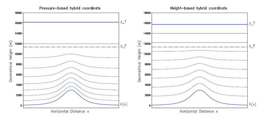
1314 CHAPTER 2. MODEL AND DATA Figure 2.1: Examples of terrain following levels, with pressure (on the right) and height (on the left) based hybrid coordinate, zT is the top of the model domain, zF is the height where the terrain following surface change to horizontal, figure from Doms et al., 2003 [30]. boundary layer turbulence to determine the intensity and type of convection. Convection is separated in shallow, deep and midlevel. A Kain-Fritsch cumulus parameterisation scheme is included as an option, here the convergence is initiated taking into account the subcloud layer convergence and the intensity is connected to CAPE. (Kain and Fritsch, 1993 [52]). For small-scale grid scales we assume that the model resolves convection by itself. Normally organized convective structures with a smaller grid spacing than 4 km could be resolved by the model; obviously convection could be activated also on smaller scales (1 km or less). We assume that with our resolution (2.8 km) we can resolve the basic aspects of convective processes using. In case of complex topography high resolution can resolve explicitly the forcing and the enhancement of convection due to the presence of the mountainous regions. The model variables are discretised on a staggered Arakawa-C/Lorenz grid with scalars defined at the centre of a grid box and the normal velocity components defined on the corresponding box faces (Fig. 2.2). In the vertical direction the COSMO atmosphere is divided in 50 layers. The centre of one layer is called level , the boundary of one layer is called half level . The principal half levels are defined from 0 at the top of the atmosphere to 50 at the soil interface (Fig. 2.1). The vertical velocity is defined at the half levels k ± 1/2 (from Schulz and Schättler, 2005 [84]). COSMO is used by DWD as the operational limited area forecast model since December 1998; its previous name was LM (Lokal-Modell). Since then, the
2.1. COSMO MODEL                                                            15

Figure 2.2: dependent COSMO variables on the Arakawa-c Lorenz grid , figure
from Doms et al., 2003 [30].

model has been improved constantly and has undergone many modifications.
In this work we have used COSMO-DE version 4.6. Until April 15, 2007, only
a version with a horizontal resolution of 7 km was operational, This model was
called LME (Lokal Modell Europa). Currently the new model, COSMO-DE,
with a resolution for the meso-γ events (∆x ∼ 2.8 km) is also operational.
The default time integration scheme is a second order leapfrog HE-VI
(horizontally explicit, vertically implicit), otherwise in this work as well as
in the operational forecast the three step Runge-Kutta scheme is used.
The new model version with high resolution (2.8km also called LMK) was
tested in many research works (i.e. Baldauf et al., 2006 [8]). The boundary
conditions are interpolated from the output of COSMO-EU (’COSMO Modell
Europa’, 7 km horizontal resolution). The further development of the COSMO
model chain are embedded in an international project. In this project (see
www.cosmo-model.org) the DWD, the German military geophysical advisory
service and the national weather services of Italy, Greece, Poland and
Switzerland are working together.
The most important differences between COSMO-EU and COSMO-DE are:

   • The horizontal resolutions are different (7km in COSMO-EU , 2.8km in
     COSMO-DE).
   • The vertical resolution change from 40 in COSMO-EU to 50 levels in
     COSMO-DE.
   • Deep convection is not parameterised any more in COSMO-DE. For
     shallow convection there is still a convection parameterisation active in
     COSMO.
   • COSMO-DE takes graupel into account as an additional microphysical
     particle.
16 CHAPTER 2. MODEL AND DATA 2.1.1 Data Assimilation in COSMO Data assimilation is a requirement for NWP. Its value increases even more for nowcasting purposes (Laroche et al., 2005 [63]). In the operational COSMO model a scheme based on the observation nudging technique has been chosen for the purpose of data assimilation. The assimilation of the radar data is realised using a latent heat nudging scheme (see Section 1.2.1). A detailed high-resolution analysis has to be produced frequently and efficiently. This requires a thorough use of synoptic and high-frequency observations. For this purpose an optimal interpolation (OI) or a 3DVAR are not optimal, since they do not allow to account for the exact observation time of synoptic data. 3DVAR and OI also neglect most of the high-frequent data unless the analysis scheme is applied very frequently, but in this case the computational costs are very expensive and the data density may become very low and inhomogeneous. Methods based on 4 dimensions offer potential advantages since they include the model dynamics in the assimilation process directly. The problem is that for the current available calculation power 4DVAR is too expensive for nowcasting. In the observation nudging technique (using atmospheric fields and some of the surface and soil fields, Doms and Schättler, 2002 [29]) for COSMO the observation processing is performed only once for each observation at the timestep when the observation is available. Thus it is a continuously assimilation scheme (see Section 1.3 for explanations). In some cases the model values and observations are combined to complement missing pieces of information, e.g. model humidity is used to convert virtual temperature measured by RASS (Radio Acoustic Sounding System) into ’observed temperature’. The nudging scheme uses the traditional data (Synop, Pilot, ...) and also precipitation derived from radar reflectivity. An observation increment is applied, which is a function of the quality of the observation; quality weights are calculated as well. The observational information contained in the observation increments and in their quality is spread explicitly to the model grid points. The assimilation scheme works for more than one grid point because if we correct the model only at one point the meteorological fields will not be smooth any more and we can create instability. In this scheme the modified model field is assumed to have an error prior to the correction. The smoothness of the meteorological fields then suggests that the corresponding model field is likely to contain a similar error in close vicinity. Hence we have to change the field near the observation taking into account the errors of the model and the errors of the field as well as their correlation. The assimilation scheme nudges the information in a certain period of
2.1.2 Initial and boundary conditions                                          17

time (assimilation window) and not only at the observation time. Thus is
accomplished by using a temporal weight function.
COSMO-DE assimilates also precipitation from the composite of the DWD
Radar network. The data has a temporal resolution of 5 minutes and a 1 km
horizontal resolution. The Radar data are interpolated onto the COSMO-
DE grid and then assimilated with a latent heat nudging scheme (Klink and
Stephan, 2004 [54], Leuenberger and Rossa, 2004 [66] and Leuenberger, 2005
[65]).

2.1.2     Initial and boundary conditions
Regional models have a high horizontal resolution that cannot be afforded in
a global model (Kalnay, 2003 [53]). Operational regional models have been
embedded or nested into coarser resolution hemispheric or global models since
the 1970s (e.g. Jones, 1973 [51]; Harrison and Elsberry 1972, [43];Chen and
Miyakoda, 1974 [19]). The lower boundary conditions are physical but at the
top and the sides they are usually artificial. For the lateral boundary condition
a periodic one (for specific scientific applications) can be used, open or inflow-
outflow boundary conditions can be used, which allow the atmosphere in the
model interior domain to interact with the external environment.
The bottom boundary conditions play an important role since the transfer
of physical properties as heat and moisture across this interface plays a
fundamental role in most mesoscale circulation phenomena (Pielke R., 1984
[80]).
In a model (in our case COSMO-DE) the information about the variables
at the lateral boundaries and their time evolution must be specified by an
external data set. These external data can be obtained by interpolation from
a forecast run of another model or from a coarser resolution run of COSMO, for
example COSMO-EU (the boundary conditions are available every hour). At
present, boundary data from the operational hydrostatic global model GME
are supported for running COSMO-EU. Time dependent relaxation boundary
conditions are used to force the solution at the lateral boundaries using the
external data.
For COSMO-DE the initial conditions are not really well defined; because
of the difference in the horizontal and vertical resolution, there is a spin-up
time of 3-6 hours, during which the humidity fluxes are adjusted to the new
topography.
18                                                CHAPTER 2. MODEL AND DATA

2.1.3     Forecast and assimilation cycle
NWP is an initial-boundary value problem; given an estimate of the present
state of the atmosphere (initial conditions) and appropriate surface and
lateral boundary conditions, the model simulates (forecasts) the atmospheric
evolution.
For the operational COSMO-DE forecast chain the four dimensional data
assimilation cycle based on a nudging analysis scheme is installed. The initial
and boundary conditions come from the COSMO-EU run, which initial and
boundary conditions come from the global model GME.
In every grid point between two different boundary conditions a linear
interpolation is made; in this way we can obtain the needed boundary
conditions for every time step. For a simple model chain scheme see Fig.
2.3.
The assimilation cycle has a routine time of 3 hours. Every hour an analysis
is written. Every 6 hours a new forecast simulation is performed; the forecast
is computed for 18 hours.

                               Boundary           Boundary           Boundary
                GME run +      conditions         conditions         conditions
                  OBS
                              obs           obs                obs            obs

                      t=0
                                    t+1              t+2                t+3
                  Initial
                                             Analysis + model                       ...
                conditions

                    Figure 2.3: Simple model chain scheme

2.1.4     Grid scale precipitation
A cloud/precipitation model is a mathematical description (a set of equations)
for the overall evolution of a cloud. These equations allow to predict
numerically the water mass in each category of hydrometeors.
The grid scale precipitation scheme in COSMO model follows a one moment
bulk formulation; the basic idea of this method is to assume as few categories
of water as necessary and to predict the total mass fraction of water in each
category.
In COSMO model different microphysical schemes are possible: from the
simplest scheme with only cloud water content (qc ) and rain water content
(qr ) to the most recent one which accounts for cloud snow (qs ), cloud ice (qi )
and the graupel phase (qg ).
2.2. RADAR DATA 19
Diagnostic and prognostic schemes are available for the rain processes
(prognostic for liquid rain and snow). In prognostic mode the full budget
equations for the precipitating hydrometeors are solved, whereas in diagnostic
mode an approximated quasi-stationary version is utilised. For high resolution
simulation, like in our case, the prognostic scheme is normally used.
The diagnostic precipitation formulation assumes a column equilibrium
for precipitating constituents; this assumption is only as an acceptable
approximation for coarse resolution. For this reason the prognostic
precipitation was introduced. For deep convection the vertical advection of
the precipitation phases must be taken into account since the air’s vertical
velocity is in the same magnitude as the fall velocity of rain and snow.
2.2 Radar data
The weather radar network of DWD consists of 16 operational Doppler
RADAR (RAdio Detection And Ranging) systems in C-Band (wavelength of
4-8 cm and a frequency of 4-8 GHz), as shown in Fig. 2.4.
The DWD uses two scanning techniques:
• In the volume scan the antenna passes through 18 different angles
of elevation from 37.0◦ to 0.5◦ every 15 minutes, thus covering the
atmosphere up to an altitude of 12 km. The volume scan consists of two
different measuring modes: the intensity mode covers the lower elevation
angles from 0.5◦ to 4.5◦ , while the Doppler mode covers the elevation
angles above. The horizontal range is 230 km for the intensity mode and
120 km for the Doppler mode.
• In the precipitation scan the lowest elevations are covered with a time
resolution of five minutes The range is 128 km and the radar beam has an
elevation between 0.5◦ and 1.8◦ depending on the orography. This scan
is made because for hydrometeorology the use of the lowest positions
(where the rain rate is estimated) has the greatest significance.
2.2.1 RY product
The RY product derived from the precipitation scan (see precedent Section), it
contains the precipitation echoes measured every 5 minutes, making very short
range forecasts of precipitation possible. This is the most important input
for our assimilation scheme. The starting point of the PIB is the observed
rain rate, which the RY product supplies based on the radar reflectivity. A20 CHAPTER 2. MODEL AND DATA
Figure 2.4: DWD radar network. The circles around each radar site have a
radius of 128km (Figure from www.dwd.de).
quality flag is used in the generation of the precipitation fields; if the quality
is insufficient in a pixel a negative value is attributed to this pixel.
Normally an empirical power-law relationship is used (R. E. Rinehart,
2004 [82]) to convert reflectivity into precipitation. This is, however, an
approximation and a source of errors. But there are also numerous others
error sources, which will be explained in the next Section.
2.2.2 Typical errors in radar precipitation estimates
Some typical problems of radar-based rainfall estimates are:
• Anomalous propagation (anaprop): In free space the path of a
radar beam (a plane electromagnetic wave) propagates straight because
dielectric permittivity ε0 and magnetic permeability µ0 are constant.2.2.2 Typical errors in radar precipitation estimates 21
The refractive index n = (µr εr )−1/2 is unity in vacuum; εr is the relative
dielectric permittivity and µr the relative magnetic permeability. If ν
is the phase velocity of radiation of a specific frequency in a specific
material, the refractive index is given by n = νc . The atmosphere’s
permittivity ε = ε0 · εr is larger than ε0 since the atmosphere is vertically
stratified, microwaves propagate at speeds ν < c. Even small variations
in the refraction index can have remarkable effects in the electromagnetic
wave propagation.
Water vapour particles have a permanent dipole momentum; therefore
its refractive index depends on the wave frequency. For microwaves the
relation can be parameterised by (following Bean and Dutton, 1968 [9]):
e e
n = K2 + K3 2 (2.1)
T T
with e the water vapour pressure in hP a, K2 and K3 are constants. If
we take into account also the dry air, with pressure Pd , we can write
Pd e e
n = K1 + K2 + K3 2 (2.2)
T T T
With K1 a constant. With some approximations applied we have:
77.6 e
n= (P + 4810 ) (2.3)
T T
With P is the total pressure in hP a.
In the troposphere the temperature and pressure profiles decrease with
the height. Since the pressure decrease is stronger than the temperature
one, n decreases with the height. Using the Snell’ s law (Fig. 2.5), the
wave front is beat downwards:
n1 sinθ1 = n2 sinθ2 (2.4)
Only the first kilometres of the atmosphere are important for most
radar meteorology applications, where the refractivity gradient is
approximately −40km−1 in standard conditions. In cases of temperature
inversion and very humid air conditions, this value can be lower than
−157km−1 , leading to anaprop (Bech et al., 1998 [10]).
• Bright band: Whether icy precipitation is from stratiform or convective
clouds, it often falls into an environment where the temperature is above
the freezing point. When snow melts into rain, radars typically observe22 CHAPTER 2. MODEL AND DATA
P n1 n2 index
v1 v2 velocity
normal θ1
O θ2
interface
Q
Figure 2.5: Refraction of light at the interface between two media of different
refractive indices, with n2 > n1 . Since the velocity is lower in the second
medium (v2 < v1 ), the angle of refraction θ2 is less than the angle of incidence
θ1
a narrow horizontal layer of stronger radar reflectivity that has been
termed the bright band (Atlas, 1990 [7]).
The falling snowflakes are crossing the 0◦ C layer and melt from the
outside. The reflectivity maximum is explained by the difference in the
value of the dielectric factor of water and ice: when a water film begins
to form on a melting snowflake, its radar reflectivity may increase by
as much as 6.5 dB. The reflectivity decreases again below the melting
level when the flakes collapse into raindrops; their fall velocities increase
causing a decrease in the number of precipitation particles per unit
volume. The size of the particles also becomes smaller in the melting
process, as their density increases from that of the snow and melting
snow to that of liquid water.
In case of strong convective currents, showers and thunderstorms tend to
destroy the horizontal stratification essential for creating and sustaining
the bright band. Normally the presence of the bright-band near the
melting level is a signature that helps to distinguish convective mode
from stratiform mode (Llsat et al., 2004 ).
• Attenuation: The intensity of electromagnetic radiation decreases due
to attenuation, when passing through a medium (e.g. atmosphere, cloud,
rain ...). This loss of radar energy is due to scattering and absorption.
Because of attenuation, storms close to the radar are better sampled than
storms far from the radar site. Small wavelength radar beams (i.e. X-
band) attenuate more rapidly than long wavelength radar (i.e. S-band).2.2.3 The composite 23
2.2.3 The composite
The composite products, e. g. by DWD, are more complicated then a simply
assemblage of separate parts. In the overlapping areas of several radar sites
the value with the best quality is selected. If the quality is the same then the
one with the strongest signal is chosen.
The data of the national composite of DWD are exchanged with the data
of the meteorological services of others European states (Belgium, Denmark,
Austria, Switzerland, France, the Netherlands, Great Britain and the Czech
Republic); in this way it is possible to build an international composite image.
Unfortunately these data was not available for the current study.
2.3 Satellite data
In our work we need information about the cloud top height. For this reason we
use products of the Satellite Application Facility on support to NoWCasting
and Very Short-Range Forecasting (SAFNWC) (for further information see
the SAFNWC manual, [72]). The SAFNWC products are based on the MSG
SEVIRI data, generate by DWD and available with a temporal resolution of
15 min.
Figure 2.6: CTTH data, image from http://nwcsaf.inm.es/
The general objective of the SAFNWC is to provide operational services to
ensure the optimum use of meteorological satellite data in Nowcasting and
Very Short Range Forecasting to the targeted users. In our case we will use
the data in order to define the cloud top height.
We use CTTH (Cloud Top Temperature and Height) and CT (Cloud Type).24 CHAPTER 2. MODEL AND DATA
2.3.1 Cloud top temperature and height
This product contains information about the cloud top temperature and height
for all pixels identified as cloudy in the satellite scene.
For its determination the following process is applied:
• The RTTOV (Rapid Transmissions for TOVS 1 ) radiative transfer model
is implemented using NWP temperature and humidity vertical profile to
simulate 6.2µm, 7.3µm, 10.8µm, and 12.0µm cloud free and overcast
(clouds successively on each RTTOV vertical pressure levels) radiances
and brightness temperatures.
• Different techniques are employed for different cloud types in order to
retrieve the best approximation for the cloud top pressure. The cloud
top temperature is linear by interpolated using the temperature of the
two nearest pressure levels in the vertical profile.
• General modules for pressure are used in order to define the cloud top
height.
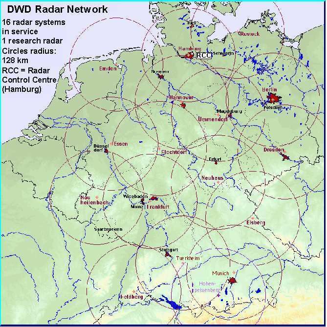
2.3.2 Cloud type
The CT algorithm provides a detailed cloud analysis; it may be used as input
to an objective meso-scale analysis, as an intermediate product input to other
products, or as a final image product. The CT product is also applied in the
calculation of cloud top temperature and height. Different channels are used
to determine CTTH depending on cloud type.
The CT classification algorithm is based on a sequence of thresholds tests; the
cloud phase flag is not yet available.
The CT selects one of the following twenty-one categories :
1) not processed containing no data or corrupted data
2) cloud free land
3) cloud free sea
4) land contaminated by snow
5) sea contaminated by snow/ice
6) very low and cumuliform clouds
7) very low and stratiform clouds
8) low and cumuliform clouds
9) low and stratiform clouds
1
TOVS instruments provide information on mainly vertical temperature and moisture
distribution2.3.2 Cloud type 25
Figure 2.7: CT data, image from http://nwcsaf.inm.es/
10) medium and cumuliform clouds
11) medium and stratiform clouds
12) high opaque and cumuliform clouds
13) high opaque and stratiform clouds
14) very high opaque and cumuliform clouds
15) high opaque and stratiform clouds
16) high semitransparent thin clouds
17) high semitransparent thick clouds
18) high semitransparent above low or medium clouds
19) fractional clouds (sub-pixel water clouds)
20) undefined by cloud mask
The algorithm for the cloud type has some typical problems: e. g. low clouds
surmounted by thin cirrus may be classified as medium clouds, very thin cirrus
can be classified as fractional clouds and very low clouds (pressure larger than
800hPa) in a strong thermal inversion may be classified as medium clouds
(pressure between 450hPa and 650hPa).26 CHAPTER 2. MODEL AND DATA
Chapter 3

The PIB algorithm

Horizontal humidity flux convergences in the lower part of a cloud tend to
trigger updrafts and cumulus convection (Xi and Reuter, 1996 [102]). The
result from many experimental studies (see Cotton and Anthes, 1989 [20]) was
that the two quantities, which are best correlated with convective precipitation,
are upward motion and moisture convergence. In his work, G. Haase (2002 [41])
asserts that in this context instability of atmospheric stratification is secondary.
He investigated the relationship between stability indices (calculated from
model variables) and precipitation; and did not find a direct connection.
The starting point of PIB (Physical Initialisation Bonn) is the analysis of the
rain field using model precipitation and the rain rate product from the radar
composite of the DWD (see Section 2.2.1). Satellite data (Section 2.3) are
used in a simple cloud model; the PIB connects the observation space directly
with model space.
A simplified precipitation scheme connects the observation space with model
space. The vertical wind and the humidity are computed from this scheme.
The main difference between the original PIB developed by G. Haase and
the current one is in the use of satellite data (SAFNWC see section 2.3)
leading to a different definition of the cloud top and to the assimilation of
non precipitating clouds. In addition we use a different definition of cloud
base and of the analysed precipitation. We introduced a mixed phase and a
more flexible definition for the conversion efficiency of saturated water vapour
into rain. In the original version it was defined at the first time step for the
whole simulated area.
In this Chapter we describe the PIB algorithm including the data processing
from the analysed precipitation (Section 3.1) to the modification of COSMO
variables (Section 3.4). In Sections 3.2 and 3.3 the assumed precipitation
scheme and the cloud model are described. A scheme of the PIB algorithm is

                                        27
28 CHAPTER 3. THE PIB ALGORITHM
shown in Fig. 3.5.
3.1 Analysed precipitation
For the determination of the analysed precipitation the first step is the
measurement of the observed precipitation. After that the scheme attributes
a time weight to the analysed precipitation.
For the formulation of the observed precipitation at every time step and for
every grid point a linear interpolation between the adjacent measurements to
the current model time step is made. The scheme takes into account only the
radar data in a time range of 10 minutes (5 before and 5 after the current time
step).
Upon the availability of radar observation directly after the current model time
step and before it, the time weight (α, eq. 3.1) is set to one. In other cases the
time weight is reduced depending on the time distance of the observation to
the current time step. In other words, if one measurement is missing either at
the last or the following observation time, the available data is used but with
a reduced α depending on the difference between the observation time and the
current model time.
In COSMO model we use the prognostic precipitation scheme where
precipitation can be horizontally advected when falling from the cloud base
to the surface. Thus the position of the precipitation at the soil can be shifted
relative to the cloud base. The position of the observed precipitation is defined
at the height of the lowest radar beam which can be approximated by the cloud
base. We avoid this problem, due to the use of different heights, by using the
model precipitation at the cloud base.
For every time step and every grid point the analysed precipitation Rana is
calculated using:
Rana = αRrad + (1. − α)Rmod (3.1)
Rrad is the radar precipitation flux and Rmod the model precipitation flux.
The model rainfall rates are provided by the COSMO grid-scale cloud and
precipitation scheme. If α is small (large), Rana is approximated by Rmod
(Rrad ). Radar data and model field are mixed only if the temporal availability
of observations is inadequate. In this case measurements can be merged partly
with model values, because the latter are already affected by assimilation.
Finally, the analysed precipitation rates in [mm/h] are transformed to fluxes
in [kg · (m2 /s)−1 ] which are used by COSMO as diagnostic output. The Rana
field can now be used as input to the one-dimensional cloud model (SectionYou can also read