Is the F10.7cm - Sunspot Number relation linear and stable? Frédéric Clette* - Journal of Space Weather and Space Climate
←
→
Page content transcription
If your browser does not render page correctly, please read the page content below
J. Space Weather Space Clim. 2021, 11, 2
Ó F. Clette, Published by EDP Sciences 2021
https://doi.org/10.1051/swsc/2020071
                                                                                                                                     Available online at:
                                                                                                                                    www.swsc-journal.org
Topical Issue - Space climate: The past and future of solar activity
 RESEARCH ARTICLE                                                                                                                OPEN          ACCESS

Is the F10.7cm – Sunspot Number relation linear and stable?
Frédéric Clette*
World Data Center SILSO, Royal Observatory of Belgium, 1180 Brussels, Belgium

              Received 26 March 2020 / Accepted 18 November 2020

              Abstract – The F10.7cm radio flux and the Sunspot Number are the most widely used long-term indices of
              solar activity. They are strongly correlated, which led to the publication of many proxy relations allowing
              to convert one index onto the other. However, those existing proxies show significant disagreements, in
              particular at low solar activity. Moreover, a temporal drift was recently found in the relative scale of those
              two solar indices. Our aim is to bring a global clarification of those many issues. We compute new
              polynomial regressions up to degree 4, in order to obtain a more accurate proxy over the whole range
              of solar activity. We also study the role of temporal averaging on the regression, and we investigate the
              issue of the all-quiet F10.7 background flux. Finally, we check for any change in the F10.7–Sunspot Number
              relation over the entire period 1947–2015. We find that, with a 4th-degree polynomial, we obtain a more
              accurate proxy relation than all previous published ones, and we derive a formula giving standard errors.
              The relation is different for daily, monthly and yearly mean values, and it proves to be fully linear for raw
              non-averaged daily data. By a simple two-component model for daily values, we show how temporal
              averaging leads to non-linear proxy relations. We also show that the quiet-Sun F10.7 background is not
              absolute and actually depends on the duration of the spotless periods. Finally, we find that the F10.7cm time
              series is inhomogeneous, with an abrupt 10.5% upward jump occurring between 1980 and 1981, and
              splitting the series in two stable intervals. Our new proxy relations bring a strong improvement and show
              the importance of temporal scale for choosing the appropriate proxy and the F10.7 quiet-Sun background
              level. From historical evidence, we conclude that the 1981 jump is most likely due to a unique change
              in the F10.7 scientific team and the data processing, and that the newly re-calibrated sunspot number
              (version 2) will probably provide the only possible reference to correct this inhomogeneity.

              Keywords: Sun / solar activity / solar indices / solar irradiance (radio) / solar cycle

1 Introduction                                                                    a full revision process was undertaken in 2011 and led to a first
                                                                                  re-calibration of this multi-century series, with correction reach-
    The sunspot number (hereafter SN; symbol: SN) (Clette                         ing up to 20% (Clette et al., 2014; Clette & Lefèvre, 2016). This
et al., 2014; Clette & Lefèvre, 2016) and the F10.7cm radio flux                   re-calibration included a full re-construction of the SN from raw
(symbol: F10.7) (Tapping & Morton, 2013) are arguably the                         original data for the period 1981 to the present, while correction
most widely used solar indices to characterize the long-term                      factors were applied to the original series built by the Zürich
evolution of the solar activity cycle and of the underlying                       Observatory before 1981.
dynamo mechanism. In order to be usable over duration of                              In this article, we will take a closer look at the F10.7cm radio
decades to centuries, those indices must guarantee a long-term                    flux, which comes second in duration after the SN, among the
stability so that levels of activity at two widely spaced epochs                  global long-duration solar activity indices based on a single unin-
can be compared on exactly the same scale. F10.7cm and the                        terrupted observing and processing technique, and on a single
SN are both absolute indices. Indeed, they do not lean on exter-                  long-duration standard reference. Since the measurements of
nal references, which anyway are absent over a large part of                      the F10.7cm radio flux were started in Ottawa in 1947 (Covington,
their temporal range (410 years for the SN, and 73 years for                      1948, 1952), this new solar index proved to be highly correlated
F10.7). Instead, the index values are only based on the knowl-                    with the SN. This can be explained by the fact that the back-
edge of the different steps in their determination, from the                      ground flux, outside flaring events, is associated with the thermal
raw measurements to the data processing method. For the SN,                       free-free and gyroresonance emission of electrons trapped in
                                                                                  closed loops anchored in the active regions, and thus primarily
*
    Corresponding author: frederic.clette@oma.be                                  in their sunspots (Tapping, 1987; Tapping & Detracey, 1990;

     This is an Open Access article distributed under the terms of the Creative Commons Attribution License (https://creativecommons.org/licenses/by/4.0),
                  which permits unrestricted use, distribution, and reproduction in any medium, provided the original work is properly cited.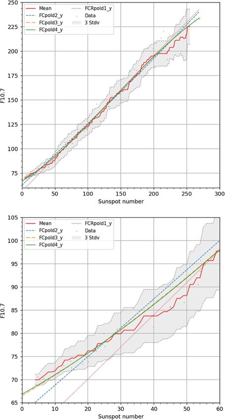
F. Clette: J. Space Weather Space Clim. 2021, 11, 2

Tapping & Zwaan, 2001). Those two indices ran in parallel over        debate, but it is generally estimated in the range between
the last 73 years and they are produced by completely different       64 and 67 solar flux units (sfu) (Tapping & Detracey, 1990;
and independent processes. Therefore, as they are supposed to         Tapping & Charrois, 1994).
retrace exactly the same evolution of the last seven solar activity       Secondly, by its definition (Wolf, 1856; Clette et al., 2014),
cycles, studying their mutual relation can give a prime diagnostic    the SN is quantized at the lowest values, as each new group
of their long-term stability. We will thus focus on the proxy rela-   (with at least one single spot), adds 11 to the index. So, for
tion between those two indices.                                       the first spot, the SN jumps from 0 directly to 11. This effect
    It turns out that, given the excellent long-term correlation      quickly decreases for values larger than 22, as contributions
between the SN and the F10.7cm radio flux, various proxy               from several groups with multiple sunspots are then combined
relations were derived over past years by different authors, or       in the total number. However, this low jump stretches the SN
they were established for operational purposes by solar data          scale near 0. As this SN feature is absent in F10.7, we can expect
services like NOAA-SWPC (Space Weather Prediction Center)             that it will break the proportionality between the two indices in
in the USA or the IPS (Ionospheric Prediction Service, part of        the lowest range.
the Bureau of Meteorology) in Australia. Those relations are              In this article, we first review all F10.7–SN proxy relations
motivated by two kinds of applications. One of them is the            published in the literature or used by operational space weather
re-construction of the F10.7 time series before the actual measure-   services. Given the mismatches between those existing proxies,
ments started in 1947. Indeed, as the sunspot number extends          we build more carefully a new least-square polynomial regres-
back over four centuries, it allows to extrapolate this radio index   sion, while exploring the effect of temporal averaging of the
over a much longer period (Svalgaard, 2016). Another applica-         source data. We also investigate the issue of the quiet-Sun
tion is producing mid-term predictions of the future evolution of     F10.7 background level. We then check the temporal stability
the F10.7cm flux. As such predictions often need to be calibrated      of the relation between F10.7 and the SN over the entire duration
and validated over many past solar cycles, they are typically         of the series. We finally conclude on the new picture emerging
based on the SN, and consequently, they produce their predic-         from our analysis and on important aspects to be taken into
tions in terms of this SN. Moreover, the number of sunspots           account for future updates of this relation between those two
and sunspot groups give a direct measure of magnetic flux emer-        most fundamental measures of the long-term solar activity.
gence at the solar surface, and is thus directly related to the           In this analysis, we use the sunspot number data provided
dynamo mechanism at work inside the Sun (Charbonneau,                 by the World Data Center SILSO (Sunspot Index and Long-
2010; Hathaway, 2010; Stenflo, 2012).                                  term Solar Observations) at http://www.sidc.be/silso/datafiles
    On the other hand, F10.7 is a chromospheric/coronal index         and the F10.7cm data series from the Dominion Radio Astrophys-
that combines two kinds of emission: gyroresonance and free-          ical Observatory, available via the Space Weather Canada
free, the latter being associated with the magnetic decay of          service at https://www.spaceweather.gc.ca/solarflux/sx-5-en.
active regions under the action of the random convection, lead-       php, and also accessible through NOAA (https://www.ngdc.
ing to the chromospheric plage component (Tapping, 1987;              noaa.gov/stp/space-weather/solar-data/solar-features/solar-radio/
Tapping & Zwaan, 2001). This is why, on timescales shorter            noontime-flux/penticton/). We use the adjusted F10.7cm flux,
than the average lifetime of individual active regions and their      which reduces the flux to a fixed distance of 1 Astronomical
associated plages, daily values of F10.7 are less correlated with     Unit (AU), and thus eliminates any annual modulation due to
the sunspot number, as first found by Vitinsky & Petrova               the orbital eccentricity of the Earth.
(1981), Vitinsky (1982), Kopecky (1982), and Kuklin (1986),
and using more modern methods by Dudok de Wit et al.
(2009, 2014). On the other hand, the daily flux offers a better        2 Past F10.7cm–SN proxy relations
proxy for ultraviolet (UV) and X-ray fluxes produced in the
chromosphere, the transition region and the solar corona. For              Quite a number of proxy relations were proposed in the
this reason, F10.7 is used by preference to the sunspot number        past. Here, we first compile all relations accessible in the
for short-term forecasts of solar irradiance in the UV to X-ray       literature or documented with associated data products at data
domain and of its influence on the Earth environment                   centers1. They are listed in Table 1, and the corresponding
(ionosphere, stratospheric temperatures, chemistry of the upper       formulae are given in Table 2. In Figure 1, we plot all those
atmosphere), and for the resulting applications (radio propaga-       proxies together, superimposed on the monthly mean values
tion, atmospheric drag on low-Earth orbiting satellites). This        of F10.7 versus SN version 2, the most recent re-calibration of
close relation with the solar UV irradiance also allows to pro-       this series (Clette & Lefèvre, 2016).
duce backward reconstructions of past UV fluxes for epochs                  So far, only a few recent proxy relations were calculated for
well before the advent of direct space-based measurements of          this new version of the SN series, SNv2 released in July 2015.
those fluxes (Svalgaard, 2016).
                                                                       1
    However, beyond their strong Sun-related similarities on             The Svalgaard-2009 proxy was found in the Web source: https://
long timescales, the two indices differ by two base characteris-      wattsupwiththat.com/2009/05/18/why-the-swpc-10-7-radio-flux-
tics that play a role primarily at the lowest levels of activity.     graph-is-wrong/. The NOAA-SWPC-2016 proxy is used for solar
                                                                      cycle predictions provided at https://www.swpc.noaa.gov/products/
Firstly, F10.7 does not fall to 0 when the Sun is spotless. A base
                                                                      predicted-sunspot-number-and-radio-flux and https://www.swpc.
background flux exists even when the Sun is fully quiet. This          noaa.gov/products/solar-cycle-progression. This proxy formula was
background emission, which corresponds to the spatially diffuse       formerly mentioned in an online document (ftp://ftp.swpc.noaa.gov/
component of F10.7, is probably associated with the small             pub/weekly/Predict.txt), which is not accessible anymore. Some
magnetic loops rooted in the quiet-Sun chromospheric network          related information can presently be found in https://www.swpc.
(Tapping & Zwaan, 2001). This lower limit is still a matter of        noaa.gov/sites/default/files/images/u2/Usr_guide.pdf.

                                                              Page 2 of 25
F. Clette: J. Space Weather Space Clim. 2021, 11, 2

Table 1. List of the proxies included in our comparison. For each proxy, we indicate the temporal granularity of the series used to fit the proxy
(day, month, year; simple means or running means), and the SN version on which the proxy was based. The label identifies the curves in the
associated figures, and the corresponding formulae are given in Table 2.

Source                                                    Temporal base                                 SN version                  Plot label
Kuklin (1984)                                             Unknown                                            1                    KU1984_V1
Holland & Vaughn (1984)                                   13-month smoothed                                  1                    HV1984_V1
Xanthakis & Poulakos (1984)                               1 day                                              1                    XP1985_V1
Hathaway et al. (2002)                                    24-month Gaussian smoothed                         1                    HA2002_V1
Zhao & Han (2008), Formula 1                              1-year mean                                        1                    ZH2008_F1
Zhao & Han (2008), Formula 3                              1-year mean                                        1                    ZH2008_F3
Svalgaard (2009)                                          1-month mean                                       1                    SV2009_V1
IPS Australia (Thompson, 2010)                            1-month mean                                       1                    IPS2011_V1
Tapping & Valdés (2011)                                   1-year mean                                        1                    T2011_V1
Johnson (2011) Formula 1 monthly                          1-month mean                                       1                    J2011_F1ma
Johnson (2011) Formula 1 yearly                           1-year mean                                        1                    J2011_F1ya
Johnson (2011) Formula 2 monthly                          1-month mean                                       1                    J2011_F2ma
Johnson (2011) Formula 2 yearly                           1-year mean                                        1                    J2011_F2y
NOAA-SWPC (2016)                                          Unknown                                            2                    NOAA_V2
Tapping and Morgan (2017) SN version 1                    10-month smoothed                                  1                    T2017_V1
Tapping & Morgan (2017) SN version 2                      10-month smoothed                                  2                    T2017_V2
Tiwari & Kumar (2018) Formula 1                           1-month mean                                       2                    TK2018_F1
Tiwari & Kumar (2018) Formula 2                           1-month mean                                       2                    TK2018_F2

Table 2. List of the proxies (labels from Table 1) and the corresponding formulae.

Plot label                                                    Formula
KU1984_V1                                                     71.74 + 0.2970 SN + 0.005146 S 2N for SN < 100.5,
                                                              104.63 + 0.3037 SN + 0.001817 S 2N for SN > 100.5
HV1984_V1                                                     67.0 + 0.97 SN + 17.6 (e  0:035S N  1)
XP1985_V1                                                     68.15 + 0.65 SN
HA2002_V1                                                     58.52 + 0.926 SN
ZH2008_F1                                                     60.1 + 0.932 SN
ZH2008_F3                                                     65.2 + 0.633 SN + 3.76  103 S 2N + 1.28  105 S 3N
SV2009_V1                                                     67.29 + 0.316 SN + 1.084  102 S 2N + 6.813  105 S 3N + 1.314  107 S 4N
IPS2011_V1                                                    67.0 + 0.572 SN + 3.31  103 S 2N  9.13  106 S 3N
T2011_V1                                                      66 + 0.446 SN ð2:  e0:027S N Þ
J2011_F1ma                                                    60.72 + 0.900 SN + 0.0002 S 2N
J2011_F1ya                                                    62.87 + 0.835 SN + 0.0005 S 2N
J2011_F2ma                                                    62.72 + (0.686 SN)1.0642
J2011_F2y                                                     64.98 + (0.582 SN)1.0970
NOAA_V2                                                       67.00 + 0.4903 SN     for SN  50;
                                                              56.06 + 0.7092 SN for SN > 50

T2017_V1                                                      67 + 0.44 SN 2:  e0:031S N

T2017_V2                                                      67 + 0.31 SN 2:  e0:019S N
TK2018_F1                                                     62.51 + 0.6422 SN
TH2018_F2                                                     65.6605 + 0.500687 SN + 1.21647  103 S 2N þ 2:71853  106 S 3N

Therefore, for converting older proxies based on SNv1 to the              second factor corresponds to a correction for an artificial infla-
SNv2 scale, we used the following re-scaling relation:                    tion of the original SN values due to the use of a weighting
                     S Nv2 ¼ S Nv1 =0:6=1:177                     ð1Þ     according to the sunspot size artificially introduced in Zürich
                                                                          (Clette et al., 2016). This was affecting all the SNv1 values after
The 0.6 factor is associated with a change of reference observer,         1946. As the F10.7 series starts in 1947, this relation is thus valid
making the former 0.6 conventional Zürich factor obsolete. The            for the entire time interval considered here. The 1.177 factor is

                                                                 Page 3 of 25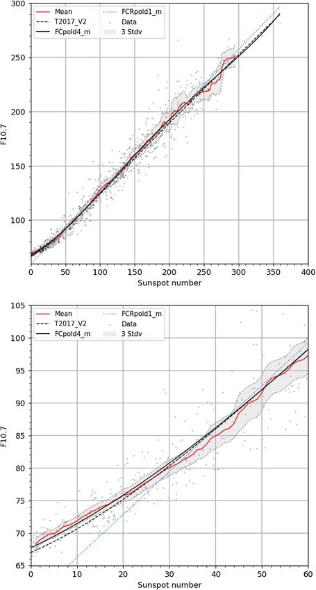
F. Clette: J. Space Weather Space Clim. 2021, 11, 2

Fig. 1. Combined plot of past published proxy relations giving F10.7     Fig. 2. Combined plot of past published proxy relations giving F10.7
as a function of the sunspot number. The curves are labeled              as a function of the sunspot number: close-up view of the low-
according to the identification in column 4 of Table 1. The curves are    activity range of Figure 1. The curves are labeled according to the
superimposed on the observed monthly mean values (gray dots).            identification in column 4 of Table 1. The curves are superimposed
                                                                         on the observed monthly mean values (gray dots).

in fact an asymptotic value reached for medium to high levels of
solar activity. It is thus variable at low solar activity, dropping to   purely empirically, and they do not explain how they were
almost 1 near cycle minima. Therefore, Equation (1) is not fully         adjusted on the data. Both proxies are shown in Figure 3.
accurate for low-activity values. Still, in our analysis presented       One can see that the SNv1 and SNv2 proxies are almost identical,
below, we did not find any significant deviation between                   indicating that the conversion in Equation (1) is accurate.
version 1 and version 2 proxies due to this effect, at the level         However, we note that all those proxies reach a value of
of precision associated with the data themselves. This can be            67 sfu for SN = 0, while almost all observed F10.7 values are
seen in the closeup view (Fig. 2).                                       above this lower limit. In fact, below in Section 6, we find that
     Overall, we observe that some proxies are very crude. They          the most probable F10.7 value for a spotless Sun is 70.5 sfu. This
are simple linear fits, ignoring the visible deviation from linear-       mismatch indicates that this part of the curve was not derived by
ity at the lower end of the range. Strong deviations also appear         least-squares but was adjusted empirically to reach exactly a
at the high values, in particular for non-linear fits (polynomial or      tie-point at 67 sfu, chosen as base quiet-Sun background when
exponential models). This can be explained by the limited                SN = 0. Given the mismatch with the actual data, this choice
number of such high values in the past solar activity record,            seems questionable. Indeed, for real applications, users need
which thus leads to large uncertainties. We also note that in            the most probable F10.7 flux, and not the lowest possible value,
the low range below SN = 20, virtually all proxies fall below            which is rarely reached. In Section 6, we will consider more
the observed values, and thus lead to systematic underestimates          closely the properties of this quiet-Sun F10.7 background.
of the average F10.7 flux at low activity.                                    Still, the other published proxies are underestimating even
     Moreover, some proxies were derived using monthly means             more the F10.7 flux at low activity. Therefore, overall, none of
or yearly means. In that case, the upper range of values is more         the proxies proposed so far are providing a satisfactory repre-
limited, and the fits should not be trusted beyond their calibra-         sentation of the relation at low solar activity. Moreover, we note
tion range. Unfortunately, while a few estimates of the error of         that all past proxies used classical least-square fits, which
individual daily F10.7 flux values were published (Nicolet &              assume that errors are present only in the fitted measurement
Bossy, 1985; Tapping & Charrois, 1994), we must note that                (here F10.7), while the other quantity (SN) is considered as a
most of the available proxy relations are given without any esti-        parameter (without error). As SN is also affected by errors, this
mate of their uncertainties, and often without clear indication of       fitting model may thus lead to systematic biases. We also
the calibration range. Here, we conservatively derived the mean          checked this aspect as explained in Section 5.2.
and standard deviation of all proxy models shown in the plot
(black line and shaded band in Fig. 3), to get a rough first idea
of their actual uncertainty.                                             3 Mean profiles
     The proxies giving the best fit to the non-linear section at
low SN are those published by Tapping & Valdés (2011) (based                 In order to extract the F10.7/SN relation without any paramet-
on SNv1) and Tapping & Morgan (2017) (based on SNv1 and                  ric model, we first derive the mean of F10.7 values and rm, the
SNv2). The authors mention that those proxies were defined                Standard Error of the Mean (SEM), for a given value of SN.

                                                                 Page 4 of 25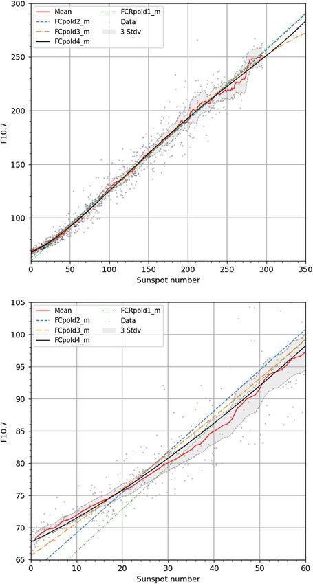
F. Clette: J. Space Weather Space Clim. 2021, 11, 2

                                                                               Figures 4–6 show the resulting mean curves and 3-rm band
                                                                          for the daily, monthly, and yearly calculations. While the
                                                                          standard deviation of the base daily data is quite large, in partic-
                                                                          ular for raw daily values (16.7 sfu overall), the SEM value is
                                                                          rather small in the low and medium range (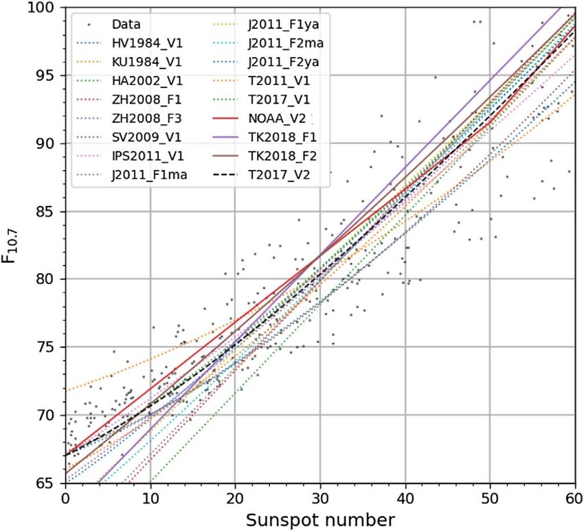
F. Clette: J. Space Weather Space Clim. 2021, 11, 2

Fig. 4. Mean non-parametric profile (red line) with 3-rm range (gray shading), obtained by averaging all daily F10.7 values for SN within a
narrow band centered on the SN in the bottom axis (see details in the main text). Gray dots are the daily observed values. The number of data
points strongly decreases above SN = 300 and F10.7 = 250 sfu, leading to a much larger SEM rm.

marginally significant, and a fully linear relation remains valid        – F10.7 and the SN are fully proportional over the full range
up to the highest observed F10.7 fluxes.                                   of observed values, and this proportionality continues
    When zooming in on the low values (Figs. 8–10), we find                down to an almost spotless Sun. This suggests that the
that the means for monthly, smoothed and yearly data start to             variability of F10.7 is entirely determined by the level of
deviate from the main linear part for SN values below an inflec-           magnetic activity also controlling the number of sunspots,
tion point at about SN = 35 (monthly values) or 50 (smoothed              without any other contribution to the radio flux. The excess
and yearly values). As there are almost no monthly or yearly              associated with the presence of spots becomes negligible
periods with a 0 mean SN, the ordinate at SN = 0 can only be              relative to the F10.7 flux distribution for a fully spotless
extrapolated, and cannot be trusted. Only for monthly means,              Sun only below SN = 8. In other words, the distribution
we find that the means tend toward 68 sfu for SN below 5.                  of the F10.7 is largely the same for a fully spotless Sun
    On the other hand, for raw daily values, we find that the              and when a single isolated and short-lived spot is present.
means continue to follow linear proportionality down to very              On the other hand, once the number of spots grows beyond
low values, around SN = 5. There are only a very few points               one (one group with a single spot), F10.7 increases fully
between 11 and 0, but at SN = 0, the mean value is well defined            proportionally with the sunspot number. So, in that sense,
at 70.5 sfu. We find that the means reach this value within the            the quantization of the SN at low activity (the 0–11 jump)
uncertainties for SN = 8, which is very low.                              does not lead to a significant non-linearity between the two
    We can thus draw three important conclusions:                         quantities, except for the values at SN = 0.

                                                               Page 6 of 25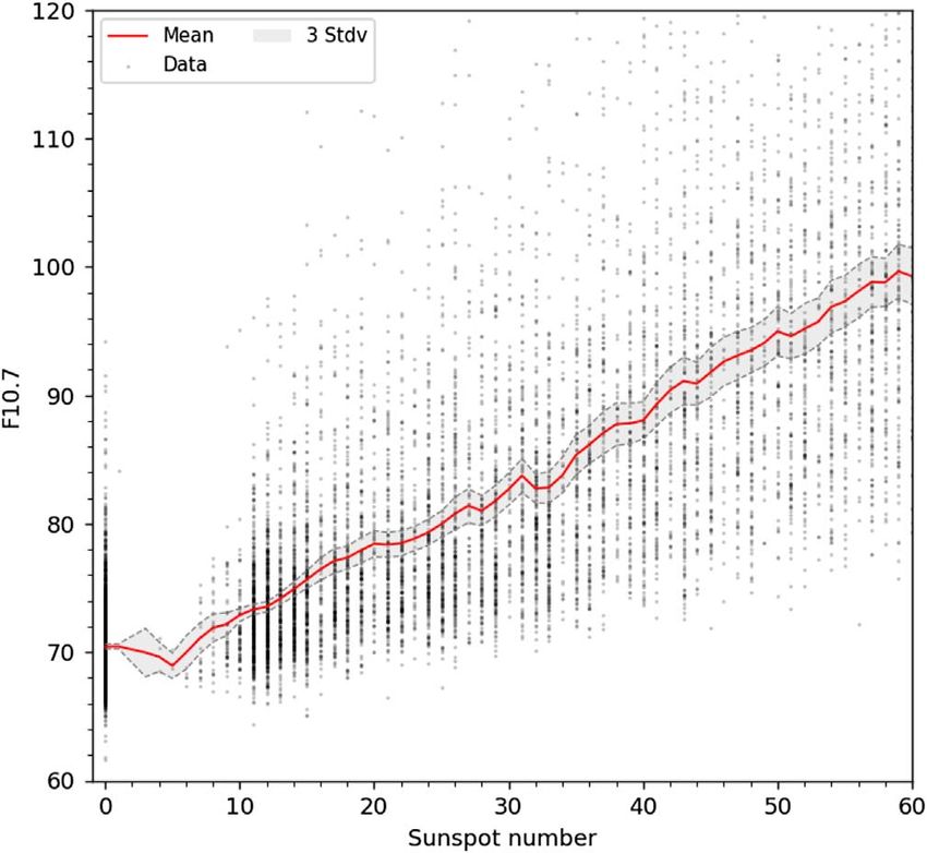
F. Clette: J. Space Weather Space Clim. 2021, 11, 2

                                                                      Fig. 7. Histogram of the ratio between daily F10.7 data and the mean
                                                                      F10.7 value (after subtraction of a 67 sfu base quiet-Sun flux), for all
                                                                      data with SN > 15. The black curve is for the entire data series, while
Fig. 5. Mean non-parametric profile (red line) with 3-rm range (gray   the blue and red histograms are respectively for the maxima of the
shading), like in Figure 4 but obtained by averaging monthly mean     solar cycles (time of maximum 2 to +3 years) and the minima (the
F10.7 values over narrow SN bands. Gray dots are the monthly mean     rest of the data). The distributions are slightly asymmetrical with a
observed values.                                                      longer upper wing. The means of the distributions are indicated by
                                                                      thick vertical lines, with the matching colors. The standard deviation
                                                                      of the distributions equals 35%, while the SEM equals 0.5% (based
                                                                      on more than 10,000 daily ratios in each distribution). The
                                                                      distributions for cycle maxima and minima are significantly shifted
                                                                      by 12% above and below the global mean.

Fig. 6. Mean non-parametric profile (red line) with 3-rm range (gray
shading), like in Figure 4 but obtained by averaging yearly mean
F10.7 values over narrow SN bands. Gray dots are the yearly mean
observed values.

                                                                      Fig. 8. Mean non-parametric profile (red line) with 3-rm range (gray
– As in temporal means, solar activity varies during the              shading) for daily values: enlarged view of the low activity part of
  chosen time interval, the linear relation will be changed           Figure 4.
  near the origin, essentially because of this single deviating
  point at SN = 0. As the latter is above the overall linear
  trend, the means will be pushed upwards, and this effect               proportion of spotless days, dominated by the F10.7 = 70.5
  will increase as the mean SN decreases toward 0. Indeed,               sfu background. This is exactly what we find in monthly,
  the time interval used for each mean will contain a growing            smoothed and yearly means, with the non-linearity

                                                              Page 7 of 25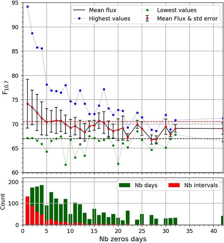
F. Clette: J. Space Weather Space Clim. 2021, 11, 2

Fig. 9. Mean non-parametric profile (red line) with 3-rm range (gray
shading) for monthly means: enlarged view of the low activity part of
Figure 5.

                                                                        Fig. 11. Polynomial of order 1 (linear fit) to 4 fitted to the monthly
                                                                        mean data by ordinary least-square regression (OLS). The curves are
                                                                        superimposed on the corresponding non-parametric mean (cf. Fig. 5)
                                                                        to show the agreement within 3-rm, and on the base data (gray dots).
                                                                        The lower plot is a close-up view of the low range of the upper plot.
Fig. 10. Mean non-parametric profile (red line) with 3-rm range
(gray shading) for yearly means: enlarged view of the low activity
part of Figure 6.                                                       4 New high-degree polynomial fits
                                                                        4.1 Ordinary least-square polynomial fit: monthly
  extending progressively to higher minimum SN as the                       means
  duration of the temporal averaging increases. In Section 7,
  we will build a simulation to validate this interpretation.               In order to obtain a better fit to the data than the earlier,
– The proxy relation is consistent with Gaussian statistics             sometimes very crude, fits shown in Section 2, we fitted poly-
  and is stable only for timescales equal to or longer than             nomials with degrees up to 4 by least-square regression of
  one month. Daily data and short timescales include an                 F10.7 versus SN. Indeed, the non-parametric mean curves
  excess of high fluxes, which varies with the solar cycle.              shown in the previous section indicate that the actual relation
  Those data are thus inappropriate for building a reliable             is largely linear over a wide range, with a rather sharp
  proxy relation.                                                       bifurcation toward a constant background in the low range.

                                                                Page 8 of 25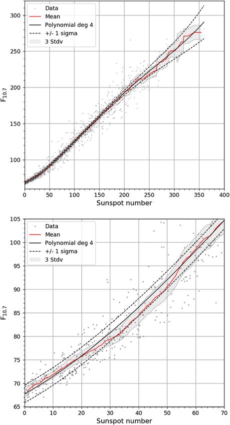
F. Clette: J. Space Weather Space Clim. 2021, 11, 2
Table 3. Coefficients of polynomials of order 1–4 fitted by the ordinary least-square regression on the monthly mean values. The coefficients
Cn correspond to Equation (2), with their standard error rn.
Coefficients Order 1 Order 2 Order 3 Order 4
(FCpol1_m) (FCpol2_m) (FCpol3_m) (FCpol4_m)
C0 62.31 62.87 65.64 67.73
r0 0.5743 0.7692 0.9457 1.134
C1 0.6432 0.6279 0.4918 0.3368
r1 4.528 103 1.478 102 3.132 102 5.649 102
C2 6.141 105 1.304 103 3.690 103
r2 5.637 105 2.592 104 7.699 104
C3 2.919 106 1.517 105
r3 5.946 107 3.773 106
C4 1.974 108
r4 6.003 109
The polynomials are of the form (here for a 4th degree Table 4. Coefficients of the linear fits to the monthly mean data in
polynomial): the restricted linear range SN = 25–290 by ordinary least-squares and
by orthogonal distance regression. The two fits match closely.
F 10:7 ¼ C 0 þ C 1 S N þ C 1 S 2N þ C 1 S 3N þ C 1 S 4N : ð2Þ
Coefficients Order 1 Order 1 (ODR)
(FCRpol1_m)
In Figure 11, we show the fits to the monthly mean values for
degrees 1 (linear) to 4. As we know that the relation becomes C0 59.66 58.21
strongly non-linear below SN = 25, the linear fit (degree 1) r0 0.8801 0.8831
C1 0.6601 0.6720
was applied to a restricted range without the interval SN = 0–
r1 6.313 103 6.338 103
25. So, this fit gives a good model for the main linear
section.
From SN = 30–250, all fits are almost identical and remain
within the uncertainty range of the mean values (gray shaded fit as order 3. Although the fits on yearly means are slightly
band). Only above 250, there is a slight deviation, with the different from the fits derived from monthly mean values, both
higher degrees falling below the linear fit. But this is hardly are compatible within the uncertainties in yearly means. This
significant, given the low number of data points in this upper difference is due to a lower non-linearity and the slightly wider
range. This is confirmed by the fact that coefficients of the range over which the relation is non-linear for yearly means, but
high-degree terms are only marginally significant. In particular is hardly significant.
for the degree-2 polynomial, only the linear term (degree 1) is
significant. This curve indeed gives the worst fit to the data. 4.3 Polynomial fits to daily values
This can be seen in the close-up view of the low part
(second plot), which shows that the fitted curve match progres- Based on Section 3, we may expect slightly different results
sively better the curved lowest part of as the polynomial degree for daily values. The polynomial and linear regressions are
increases. Only the 4th-degree polynomial closely reproduces shown in Figure 13 and the coefficients are listed in Tables 7
the low part and remains within the uncertainty of the mean and 8. We find that for the main linear range up to SN = 250,
values. The coefficients for fitted polynomials up to degree 4 the different fits match closely, like for yearly and monthly
are listed in Table 3. means. They then diverge from each other at higher values,
As the relation between the two indices is fully linear over a which is again due to the steeply decreasing number of data
wide range, in this case above SN = 25, we also derived the points in this upper range. The non-linear fits at order 2–4 tend
linear fits to this linear section. The coefficients are given in to fall below the linear fit, aligning better with the mean
Table 4 (also for the orthogonal regression method described values. However, the linear fit still falls within the uncertainty
in Sect. 5.2). The linearity is confirmed by the fact that polyno- range. So, the differences brought by higher degrees are not fully
mials fits above degree 1 do not give stable solutions, once the significant. This is again confirmed by the low level of signifi-
lowest range is excluded (terms of degrees above 1 are not cance of polynomial coefficients with degrees higher than 1.
significant). The low range is where the situation differs markedly from
the monthly and yearly mean analyses. Here (Fig. 13), the linear
4.2 Polynomial fits to yearly means fit (over the range above SN = 25) remains close to the mean
values down to the lowest values. In the low range, the
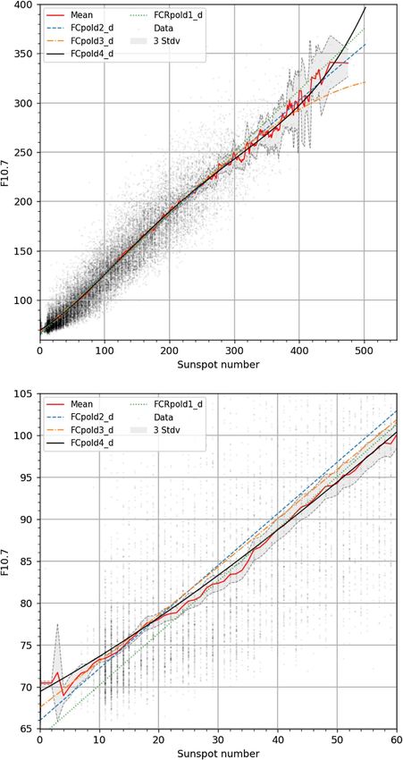
We repeated the analysis on yearly values and found largely order-4 curve again gives the best fit, although it fails for SN
the same conclusions. The curves are shown in Figure 12, and values below 6, as the mean then deviates abruptly over a very
the polynomial coefficients for the fits to yearly means are given small range. Ignoring this section, the order-3 polynomial gives
in Tables 5 and 6. the best fit overall. It reaches the mean background value for
In this case, the fit is also not significant at polynomial order SN = 0 (70.5 sfu) at SN = 5. This suggests that for SN below 6,
2, and the order 4 polynomial gives roughly the same quality of this background value can be used instead of the polynomial fit.
Page 9 of 25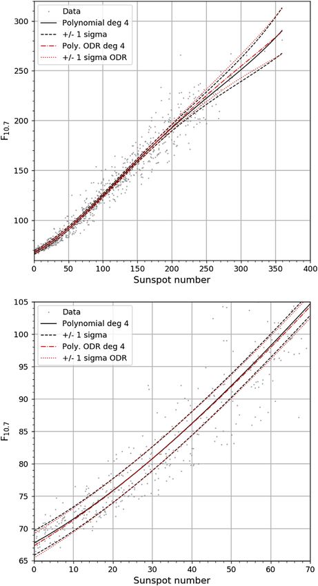
F. Clette: J. Space Weather Space Clim. 2021, 11, 2

Fig. 12. Polynomial of order 1 (linear fit) to 4 fitted to the yearly mean data by ordinary least-square regression (OLS). The curves are
superimposed on the corresponding non-parametric mean (cf. Fig. 6) to show the agreement within 3-rm, and on the base data (gray dots). The
lower plot is a close-up view of the low range of the upper plot.

                                                              Page 10 of 25
F. Clette: J. Space Weather Space Clim. 2021, 11, 2
Table 5. Coefficients of polynomials of order 1–4 fitted by the ordinary least-square regression on the yearly mean values. For the order 2 and 4
polynomials, coefficients for degree 2 and above are not significant (marked in italics), indicating that the proxy relation is essentially linear.
Coefficients Order 1 Order 2 Order 3 Order 4
(FCpol1_y) (FCpol2_y) (FCpol3_y) (FCpol4_y)
C0 61.07 62.64 66.56 66.85
r0 1.323 1.873 2.404 3.220
C1 0.6555 0.6114 0.4163 0.3942
r1 1.062 102 3.893 102 8.761 102 1.816 101
C2 1.862 104 2.129 103 2.510 103
r2 1.583 104 8.031 104 2.84 103
C3 5.081 106 7.327 106
r3 2.062 106 1.623 105
C4 4.216 109
r4 3.021 108
Table 6. Coefficients of the linear fits to the yearly mean data in the Sun, in Section 6: our polynomial fits the most probable
restricted linear range SN = 30–220 by ordinary least-squares. flux instead of the assumed F10.7 background value at SN = 0,
which is a lower boundary. Finally, we point out that our
Coefficients Order 1 4th-order polynomial is entirely defined by a least-square fit
(FCRpol1_y)
to the data, and is not attached to a predefined tie-point, like
C0 56.24 the Tapping & Morgan (2017) curve. It thus allows classical
r0 2.259 statistical tests on fitted polynomials, including the estimate of
C1 0.6936 errors on polynomial coefficients and on the resulting proxy
r1 1.739 102 values.
Therefore, the fit on daily values helps to confirm the higher
5 Polynomial error determination
linearity of the F10.7–SN relation down to very low levels. 5.1 Uncertainties on polynomial values
However, as expected, the fitted curves are significantly higher
than the fits on monthly and yearly means, due to the upward Regression methods allow to determine the standard errors
bias characterizing raw daily values (see Sect. 3). Beyond the rn on each polynomial coefficient. However, an exact derivation
linearity check, they should thus not be considered for a proxy of the standard error rp on polynomial values themselves, based
relation. on those standard errors rn, does not exist in the literature, due
to the mathematical complexity of this problem. Indeed, the
4.4 Comparison with the Tapping and Morgan (2017) errors on the coefficients for the different terms are actually
proxy inter-correlated, as they are determined together. Therefore,
the total variance of the polynomial values is not the simple
In order to check if indeed the new polynomial fits bring an naive sum of the individual variances of all terms. However,
improvement on past relations, in Figure 14, we compare the a proper estimate of rp can be derived, based on the fact that
order-4 polynomial with the best curve identified among the the actual error for each term (each degree) is the conditional
past published proxies, namely the curve by Tapping & Morgan error on that coefficient, i.e., the uncertainty of that polynomial
(2017). Here, we consider the fit on monthly means, as most of term given the values of the coefficients for all other terms
the fits are based on temporally averaged numbers, in order to (in the solution of the least-square regression). In order to
smooth out the random variations due to short-timescale solar estimate this conditional error, we can make a regression for
variations. only one term (one polynomial degree) at a time, after sub-
One can see that both fits match very closely, within 4 sfu tracting all other terms from the original observed F10.7 values,
over the whole linear range. The slope is slightly lower than with the other coefficients set at the values given by the
the slope of a purely linear fit on the range SN = 25–290 (dotted regression.
line). This may be due to the influence of the upward deviation In order to simplify this calculation, we considered that, as
for SN below 30. we go to higher degree terms, their contribution becomes smal-
Now, looking at the lowest range, we find that the ler. Therefore, we derived the conditional error for each degree
4th-degree polynomial tracks the data slightly better, and at least n by regressing for each degree separately (one-term model),
remain within the uncertainty range of the means, contrary to after subtracting successively all polynomial contributions of
the relation by Tapping & Morgan (2017), which is too low. lower degrees (F. Clette: J. Space Weather Space Clim. 2021, 11, 2
Fig. 13. Polynomial of order 1 (linear fit) to 4 fitted to the daily data by ordinary least-square regression (OLS). The curves are superimposed
on the corresponding non-parametric mean (cf. Fig. 4) to show the agreement within 3-rm, and on the base data (gray dots). The lower plot is a
close-up view of the low range of the upper plot.
Page 12 of 25F. Clette: J. Space Weather Space Clim. 2021, 11, 2
Table 7. Coefficients of polynomials of order 1–4 fitted by the ordinary least-square regression on the daily values. The coefficients Cn
correspond to Equation (2), with their standard error rn.
Coefficients Order 1 Order 2 Order 3 Order 4
(FCpol1_d) (FCpol2_d) (FCpol3_d) (FCpol4_d)
C0 66.72 65.97 67.52 69.41
r0 0.1654 0.2083 0.2430 0.2711
C1 0.6002 0.6198 0.5432 0.3938
r1 1.253 103 3.572 103 7.185 103 1.204 102
C2 7.068 105 5.561 104 2.613 103
r2 1.207 105 5.246 105 1.432 104
C3 1.260 106 1.033 105
r3 1.027 107 5.965 107
C4 1.225 108
r4 7.937 1010
Table 8. Coefficients of the linear fits to the daily data in the and also decreases for each term of a given degree n, as the
restricted linear range SN = 5–290 by ordinary least-squares and by
degree d of the polynomial increases (and thus the number of
orthogonal distance regression. The two fits match closely.
degrees of freedom in the regression).
Coefficients Order 1 Order 1 We observe that those rather simple expressions already
(FCRpol1_d) (ODR) give a very good agreement with the real data-based errors. This
rather simple empirical weighting thus probably reflects the
C0 64.79 62.23
dominant corrections associated with the inter-dependency of
r0 0.2010 0.2030
C1 0.6171 0.6419 the least-square polynomial coefficients. A mathematical
r1 1.592 103 1.610 103 demonstration goes well beyond the scope of this study, but
the good match with the data-based errors indicates that we
obtain here a reliable estimate of this polynomial error
(Fig. 15). This marks a big improvement on all previous proxy
where Cn is the coefficient to be determined (with its relations, where the error was missing and thus entirely undeter-
error) and d is the degree of the polynomial. This model is mined. Equation (5) conveniently allows a direct calculation
fitted to the F10.7 data series, minus all fitted terms of lower of the error, without requiring to re-do the above extraction of
degree: conditional errors from the data themselves. Finally, we point
X
n1 out that rTot gives the uncertainty on the proxy values, which
F corr ¼ F 10:7 C k S kn : ð4Þ combines both the errors in F10.7 and SN. This must be
k¼0 distinguished from the standard error of a single daily F10.7 mea-
surement, which is globally estimated at about 2% by Tapping
The fact that we did not subtract the terms of higher degrees and Charrois (1994). As expected for such a regression, the
leads to a slight overestimate of the residual error for each smallest errors (±2 sfu) are found in the vicinity of the mean
degree, as it also includes the residual uncertainties of all of all values, i.e., SN = 120 and F10.7 = 135 sfu, and the error
degrees above n. Therefore, the conditional errors calculated grows in both directions away from this point.
in this way for each separate degree give an upper limit.
Deriving the above errors from the data requires a statistical
5.2 Orthogonal-distance regression versus
processing and multiple regressions on the source data. So, for
ordinary least-square regression
practical applications, this approach would be too heavy. There-
fore, based on the data-based errors obtained by this procedure, In the ordinary least-square (OLS) regression, the model
we found a simple mathematical representation that gives a assumes that all errors are in the dependent variable (“response”,
good approximation of the rp errors from the full determination here F10.7) and not in the independent variable (“explanatory”,
described above, and that can be calculated directly for a here SN). As we know that in our case, both quantities are actually
polynomial value calculated at any given SN: affected by errors, we repeated the regression, but using instead
vffiffiffiffiffiffiffiffiffiffiffiffiffiffiffiffiffiffiffiffiffiffiffiffiffiffiffiffiffiffiffiffiffiffiffiffiffiffiffiffiffiffiffiffiffiffiffiffiffiffiffiffiffiffiffi
!2
u d the orthogonal distance regression (ODR) technique, which takes
uX S nN SN
n
rTot ¼ t rn ð5Þ
into account the uncertainties in both regressed variables.
n¼0 2n1 ðd þ 1 nÞ2 We find that the differences between the coefficients derived
from the ordinary and ODR regressions are within the computed
where SN is the mean of all SN values in the data set (120 uncertainties, and are thus not significant. Likewise, Figure 16
with the actual data). illustrates this close agreement for the 4th-degree polynomials
It consists in the sum of squared errors for each term, using derived by both methods. Therefore, we conclude that the
the (non-conditional) standard error on each coefficient given by ordinary regression gives valid fits in this case. This can be
the least-square regression procedure, rn, but with a weight explained by the very high level of correlation between the
factor that decreases for increasing degree n (powers of 2), two indices over long timescales.
Page 13 of 25F. Clette: J. Space Weather Space Clim. 2021, 11, 2
Fig. 14. Comparison of our 4th order polynomial with the proxy relation from Tapping and Morgan (2017). The curves are superimposed on
the corresponding non-parametric mean (cf. Fig. 5) to show the agreement within 3-rm, and on the base data (gray dots). The lower plot is a
close-up view of the low range of the upper plot.
Page 14 of 25F. Clette: J. Space Weather Space Clim. 2021, 11, 2
Fig. 15. Order-4 polynomial with uncertainty range (1 standard error Fig. 16. Comparison of 4th-degree polynomials obtained by the
rp) on polynomial values, superimposed on the corresponding non- ordinary least-square regression (OLS) and by the orthogonal-
parametric mean profile and SEM rm obtained in Section 3. The distance regression (ODR). The differences are small in comparison
lower plot is a close-up view of the low-activity range in the upper with the 1-rp standard error of the fit, and are thus not significant
plot. over the whole range of values.
different in each case, we suspected that the temporal scale
6 Background flux for a spotless Sun plays a central role.
In the above curves, we noted that past relations found by 6.1 Dependency on spotless duration
Tapping & Valdés (2011) and Tapping & Morgan (2017)
assumed a base radio flux of 67 sfu at SN = 0. By contrast, In order to investigate such a temporal effect, we extracted
our mean curves based on daily values indicate a higher mean all spotless days in the SN series, and the corresponding daily
F10.7 for all spotless days in the series, at 70.5 sfu. However, F10.7 flux. Then, we also grouped uninterrupted sequences of
the monthly means tend to converge toward lower values near contiguous spotless days. Finally, we computed the distribution
SN = 0, though still above 67 sfu. We can thus wonder how of F10.7 values for all spotless sequences of the same length in
to reconcile those apparently contradictory determinations of the observed series. Figure 17 shows the mean values, standard
the same parameter. As the underlying temporal resolution is deviations and extreme values of the F10.7cm flux for all
Page 15 of 25F. Clette: J. Space Weather Space Clim. 2021, 11, 2
sequence lengths found in the series. In the lower panel, we also
plotted the number of days included in each category, and how
many sequences were found for each duration. The longest
sequence lasted 42 days, but most spotless days sequences last
less than 10 days, with many isolated spotless days.
Our analysis shows that the mean F10.7 flux systematically
increases as the duration of a spotless-day sequence decreases.
For duration above 15 days, the most likely F10.7 value is near
68 or 69 sfu. On the other hand, it increases to 74 sfu for single
spotless days immediately surrounded by active days with one
or more sunspots. The lowest mean daily value is 67 sfu and
is reached only for 6 sequences with duration of 22, 27 and
28 days. The red dashed line at 70.5 sfu corresponds to the
mean flux for all spotless days. Quite logically, it corresponds
to the mean levels for duration 5–10 days, which is near the
mean duration of spotless intervals.
Now, considering the extreme values, we also find a steady
increase of the upper values (blue dots) with decreasing
duration, up to as high as 95 sfu for a single spotless day. Based
on the above regressions, such fluxes usually correspond to
SN values of 50, i.e. to moderate levels of activity. On the other
hand, the lowest values (green dots) do not show any
dependency on duration. They stay around the 67 sfu level, with
rare extremely low values down to 61.6 sfu (November 3,
1954). This thus validates the choice of 67 sfu as the all-quiet
base flux, shown in Figure 17 as the horizontal black dashed Fig. 17. Plot of the mean F10.7 background flux for spotless days
line. (red dots) as a function of the duration of the sequence of contiguous
Actually, there are only 33 values below 66 sfu in the whole spotless days. The errors bars correspond to one standard deviation.
series. Moreover, all 8 values below 65 sfu and 14 values out of The upper curve (blue dots) and lower curve (green dots) are the
25 between 65 and 66 sfu appear exclusively in 1953 and 1954, lowest and largest F10.7 values for each spotless duration. The red
some of them even on days when the Sun was not spotless. dashed line marks the overall mean spotless flux (70.5 sfu), while the
By contrast, the lowest values recorded after 1954 are always lower black dashed line is the mean minimum flux (67 sfu). The
above 65.5 sfu, and almost all are occurring quite logically lower panel gives the number of intervals for each spotless duration
during the longest minimum recorded in the F10.7 series, (red bar) and the number of days included in each duration (green).
between cycle 23 and 24 in 2008. By comparison, the cycle
18–19 minimum in 1954 was not particularly low and although there are a few as high as 80 sfu or more. On the other
protracted. This suggests that the record-low values in 1953– hand, there are almost no values below 67 sfu.
1954 are either spurious or suffer from a calibration problem. Such chromospheric plages are typically present just before
As indicated by Tapping (2013) and Tapping & Morgan the emergence of a first spot, or they remain after the decay of a
(2017), those early data may indeed suffer from larger errors, last sunspot. Therefore, short spotless intervals surrounded by
as the calibration method was not fully standardized, and the more active periods are most likely to show a significant excess
location in Ottawa until 1962 caused larger radio interferences. in radio emission above the lowest all-quiet level. Conversely,
Therefore, a base background flux as low as 64 sfu, as only very long spotless periods can include days without any
suggested by Tapping & Detracey (1990) and Tapping & activity features on the Earth-facing solar disk. The only small
Charrois (1994), seems doubtful and too low for the real fully active regions present just before the long spotless interval have
quiet-Sun. enough time to decay entirely, well before new bright chromo-
spheric structures develop, heralding the appearance of the first
6.2 Interpretation spots marking the end of the protracted spotless period.
Consequently, the mean background level does not have an
We can explain this dependency of the background levels absolute value, as the lowest level of 67 sfu is almost never
on the duration of spotless intervals by the presence of other reached, even when there are no sunspots. We can thus expect
sources of F10.7 emission, even when there are no associated to see a dependency of the asymptotic F10.7 value near SN = 0
sunspots. This includes various features in the chromosphere when applying a temporal averaging to the raw daily data series.
and lower corona associated with closed magnetic fields weaker Without any averaging or when the averaging duration is short,
than those concentrated in sunspots, like bright chromospheric days in long spotless intervals are mixed with those in short
plages, filaments, coronal condensations (Shimojo et al., 2006; intervals, leading to a higher mean, rising to 70.5 sfu for
Ermolli et al., 2014; Schonfeld et al., 2015; Pevtsov et al., 1-day timescale. At the other extreme, averaging over very
2014). In particular, when the Sun is very quiet (few isolated long-duration, like one year, inevitably mixes spotless periods
spots) or entirely spotless, the associated plages have a small with active periods, as virtually no spotless periods have
extent but still contribute a significant excess in F10.7. Indeed, duration above about 30 days. Therefore, the lowest F10.7 yearly
Figure 17 shows that most of the values are below 80 sfu, mean values are expected to be also higher than the 67 sfu
Page 16 of 25F. Clette: J. Space Weather Space Clim. 2021, 11, 2
minimum. It turns out that a duration of one month best
matches the actual duration range of spotless episodes. Monthly
means are thus best for recording the lowest possible mean
radio fluxes of the fully quiet Sun.
Finally, we note that this chromospheric background inter-
pretation agrees with the identification of two types of emission
sources for F10.7 (Tapping, 1987; Tapping & Detracey, 1990;
Tapping & Zwaan, 2001; Tapping & Morton, 2013; Schonfeld
et al., 2015). While the gyroresonance emission is closely
associated with strong magnetic fields in sunspots (>300 G), a
so-called “diffuse” component by free-free thermal emission
is attributed to plages and the overall chromospheric network.
The latter is the best candidate for the variable background flux
diagnosed here. In this respect, we note that while the sunspot
component of F10.7 will track instantaneously the evolution of
active regions (fully linear relation), the plage component will
be extended and delayed in time relative to the associated
sunspots, as it corresponds to the progressive decay and disper-
sal of flux emerging in active regions.
Therefore, the dependency between the mean background
flux and the duration of the spotless interval is consistent
with this interpretation, and offers an independent indicator of Fig. 18. Model of the monthly temporal averaging of daily data built
this dual-source nature of the F10.7cm radio flux. It also implies from two components: linear component and constant lower
that the disagreements between F10.7 and the SN are probably background at 70.5 sfu. The pink crosses are the synthesized daily
due for a significant part to the time delay intrinsic to the values. The green dots are the corresponding monthly mean values,
free-free emission from plages, rather than simply to a non- and the blue line is the non-parametric local mean of those values. As
proportionality with the underlying emerging magnetic fluxes, a comparison, the black line is the 4th-order polynomial fitted to the
and thus with the SN. Indeed, the latter is only sensitive to real monthly mean data (Table 3), with uncertainties (black dashes
strong fluxes freshly emerged in sunspots, without mixing with lines).
a second magnetic-decay component. The fact that disagree-
ments between those two indices increase for short time scales,
below one solar rotation and thus below the average plage life- 1. For most of of the range, we used the linear fit to the lin-
time, also concurs with the prominent role of this temporally- ear part of the data (from Table 8).
smeared weak-field component. 2. For the lowest SN values, when the linear relation falls
below the base F10.7 background, chosen at 70.5 sfu,
the output value is set at the constant value of 70.5 sfu.
An alternate model for this background flux can take into
7 A simple model for the the F10.7/SN account the fact that the mean background is not constant
non-linearity but increases even when the Sun is spotless, up to 74 sfu,
as demonstrated in Section 6.
In the above analyses, we found that daily values indicate
that the relation between F10.7 and SN is linear almost down We then applied the usual monthly and yearly averaging to
to the lowest values of SN = 11 (single isolated spot). Only this synthetic series.
for smaller SN values close to 0, F10.7 stops decreasing and In Figure 18, the model for daily values assumes a constant
reaches its background level, in the range 68–70 sfu as found background at the mean F10.7 flux for a spotless Sun (pink
in Section 6. There is a break from the linear relation, with crosses). In Figure 19, the model assumes a progressive
the last points near SN = 0 located several solar flux units above rise of the F10.7 flux over the range found in our above analysis
the linear relation, which intercepts the axis at SN = 0 at a value of the base flux according to the duration of the spotless
of 58 to 62 sfu (see Tables 3–7). period. It starts from 69 sfu, the low value for a fully spotless
When deriving monthly or yearly means, the averaging Sun and rises to 75 sfu, the upper value found for isolated spot-
interval inevitably includes periods of different activity levels, less days. This can be considered as representative of the flux
including some inactive days, when F10.7 is at its lowest level when just one isolated sunspot group is present on the Sun.
and thus shows an excess relative to a purely linear relation. Here, this ramp connects with the main linear relation at about
As the mean activity during the averaging interval decreases, SN = 24.
the proportion of spotless days increases, and thus also the Our degree-4 polynomial based on the true data (black line,
fraction of points bringing an excess above the linear relation. with uncertainties as dashed lines) nicely falls in the middle of
We can thus expect a progressive upwards deviation from the simulated monthly means for both options. The agreement
linearity, like we observe in the monthly and yearly mean curves. with the mean of data values (blue curve) is best for the second
In order to simulate this scheme, we took the observed SN model, where the agreement is very tight. The first model with a
time series, and synthesized a F10.7 time series, by converting higher but uniform background gives a higher curvature below
each SN value via a two-component model: SN = 24.
Page 17 of 25F. Clette: J. Space Weather Space Clim. 2021, 11, 2
Fig. 19. Model of the monthly temporal averaging of daily data built Fig. 21. Model of the yearly temporal averaging of daily data built
from two components: linear component, and here, a slightly rising from two components: linear relation and slightly rising background
background with increasing SN. The elements of the plots are the with increasing SN. The elements of the plots are the same as in
same as in Figure 18. Figure 18.
time-averaging of the raw linear daily values can produce the
non-linear proxy relation, thus also indicating that this non-
linearity is dependent on the temporal-averaging applied to
the data before making the regression.
8 Temporal variations
So far, we included the entire duration of the time series,
thus making the assumption that both the F10.7cm flux and the
sunspot number series are homogeneous over the entire 68-year
duration included here. However, Clette et al. (2016) made a
first simple comparison between the newly released Version 2
of the sunspot number and F10.7 as a function of time, and found
a 12% upward jump in the F10.7/SN ratio, occurring between
1979 and 1983.
Likewise, by a comparison to the sunspot number series
(versions 1 and 2) and the total sunspot area, Tapping & Valdés
(2011) and Tapping & Morgan (2017) found that the F10.7 time
series shows an upward deviation in the second half of the
Fig. 20. Model of the yearly temporal averaging of daily data built series, mostly after 1980, relative to both the sunspot number
from two components: linear relation and constant lower background and sunspot areas. Although this trend is stronger when compar-
at 70.5 sfu. The elements of the plots are the same as in Figure 18, ing with SNv1, it is still present when SNv2 is taken as reference.
with green dots and curve corresponding to yearly averages and the The authors fit a smooth curve as a function of time over the
polynomial also to yearly mean data (Table 5). whole duration of the series, and they interpret the resulting
global trend as a real change in solar properties. This evolution
would parallel the overall decline of solar cycle amplitudes
We also made the simulations using yearly means (Fig. 20 since the mid-20th century, thus invoking a possible genuine
and 21). They also give a good agreement, but given the lower change in the properties of the Sun.
number of points and slightly more linear relation, the monthly
simulations shown here illustrate more clearly how temporal 8.1 A transition between two stable periods
averaging is producing a curvature of the relation.
Overall, those two very simple simulations match strikingly In order to check for such a change in the relation between
well the actual data. They thus confirm the mechanism by which the two measurements, we used the 13-month smoothed
Page 18 of 25F. Clette: J. Space Weather Space Clim. 2021, 11, 2
Fig. 22. Plot of F10.7 versus SN, using the original SN series (version Fig. 23. Plot of F10.7 versus SN, equivalent to Figure 22 but using the
1). The data are smoothed by a 13-month running mean. The line new re-calibrated version of the SN series (version 2). The data are
connects successive months, and thus illustrate the chronological smoothed by a 13-month running mean. The data curve is in blue or
evolution. The curve is colored in blue or red for dates before and red for dates before and after 1981. The black lines correspond to
after 1981. linear fits to the entire series (solid line), the period before 1980
(dotted) and the period after 1980 (dashed).
monthly means, using the classical Zürich smoothing function. is thus characterized by a single jump separating two fully
This allows to reject random fluctuations associated with solar homogeneous periods, during which the F10.7/SN relation is
activity at time scales shorted than one year, while retaining a very stable.
better temporal sampling than in yearly means. In our case, in For each homogeneous interval, we could then derive the
the above F10.7 versus SN representation, we checked over two corresponding linear relations using the same regression
which time interval the data follow the same relation in the methods, as applied before to the whole series (Fig. 23). For
F10.7/SN space. the period before 1980, we find a slope of 0.635 ± 6.61
In Figures 22 and 23, the resulting curves are shown respec- 103 (dotted line), while after 1980, the slope becomes steeper
tively for the SN version 1 and SN version 2. The curves now at 0.702 ± 8.87 103 (dashed line). This corresponds to an
include the chronology and consist of several narrow loops upward jump by a factor 1.106 ± 0.017, thus of about 10.5%.
corresponding to each of the solar cycles, varying from very The slope found for the entire series naturally falls in-between,
low values at minima to the maxima while staying close to a with an intermediate slope of 0.660 ± 6.313 103 (cf.
diagonal line, as can be expected given the close proportionality Table 4). The coefficients for those two linear fits are given
of the two indices, as shown in the previous sections. together with the two 4th-degree polynomial fits in Table 9.
We note that two cycles deviate strongly in the case of the Such a jump is highly significant, as Tapping & Charrois
SN version 1 (blue loops in Figure 22). They correspond to (1994) and Tapping (2013) give an accuracy of 1% for the flux
cycles 22 and 23, when SN version 1 is know to be affected measurements and of 2% for the daily index derived from the
to drifts in the Locarno pilot station (Clette et al., 2014, “spot” measurements at 20 h 00 UT.
2016). On the other hand, the agreement is much tighter with Checking the past published proxies, we note that early
SN version 2 (Fig. 23), in particular over all cycles after cycle proxies that were based only on the first part of the series, like
21 for which the SN was entirely re-constructed based on a Holland & Vaughn (1984) or the IPS formula (Table 1), match
multi-station reference. the low linear fit for the period before 1980 in Table 9, while the
We will thus now concentrate on this second comparison NOAA proxy adjusted to the recent SN version 2 (1), has a
with SN version 2. The plot immediately shows that the curves steeper slope matching well the second higher fit for the recent
are grouped along two preferential bands located above (colored period after 1980. So, the disagreements between some of the
blue) and below (red) the fit to the entire series (solid black past proxies actually originate from the temporal inhomogeneity
line), with very few points in-between, near the global fit. This of the F10.7 index itself, as diagnosed here.
indicates that the relation was actually very stable during two Another consequence is that when including the entire time
time periods and jumped directly from one relation to the other. series, the least-square regression errors will not decrease when
We then looked for the time sub-intervals following the using monthly or yearly mean values, exactly as we found in
upper and lower linear relation, and we found that the lower our global regressions (Sects. 4.1 and 4.2). We can now
relation applies to all data before 1980, while the upper relation explain it by the fact that a significant part of the deviations
is valid for the entire period after 1980. The temporal evolution of individual monthly or yearly mean values relative to the
Page 19 of 25You can also read