Variation of leading-edge-erosion relevant precipitation parameters with location and weather type
←
→
Page content transcription
If your browser does not render page correctly, please read the page content below

B      Meteorol. Z. (Contrib. Atm. Sci.), Vol. 30, No. 3, 251–269 (published online March 26, 2021)
       © 2021 The authors
                                                                                                                 Energy Meteorology

Variation of leading-edge-erosion relevant precipitation
parameters with location and weather type
Anna-Maria Tilg1∗ , Martin Hagen2 , Flemming Vejen3 and Charlotte Bay Hasager1
1
  Technical University of Denmark, Department of Wind Energy, Roskilde, Denmark
2
  Deutsches Zentrum für Luft- und Raumfahrt (DLR), Institut für Physik der Atmosphäre, Oberpfaffenhofen,
Germany
3
  Danish Meteorological Institute, Copenhagen, Denmark
(Manuscript received October 8, 2020; in revised form February 12, 2021; accepted February 14, 2021)

             Abstract
             Precipitation is a key driver of leading-edge erosion of wind turbine blades, which leads to a loss in annual
             energy production and high cost for repair of wind turbines. Precipitation type, drop size and their frequency
             are relevant parameters, but not easily available. Reflectivity-Rain Rate (Z-R) relationships as well as annual
             sums of rainfall amount and rainfall kinetic energy potentially could be used to estimate leading-edge erosion.
             Although Z-R relationships and amounts are known for several places, their spatial variation and dependence
             on weather types is unknown in the North Sea and Baltic Sea area. We analysed time series of multiple
             disdrometers located on the coast of the North Sea and Baltic Sea to characterize the variation and weather-
             type dependence of the Z-R relationship, precipitation type, rainfall amount and kinetic energy.
                 The Z-R relationship as indication for the mean drop-size distribution showed small variations within
             different locations, but had a large variability for specific, but rare weather types. Only the precipitation types
             snow and hail showed some tendencies of weather-type dependence. Rainfall amount and rainfall kinetic
             energy were higher for stations in the eastern part of the North Sea compared to the western part and the
             Baltic Sea. Highest values were related to advection from the West. Overall, variations with location and
             weather type were found. These results will need to be considered in leading-edge erosion modelling and site
             assessment.
             Keywords: Z-R relationship, Rainfall kinetic energy, North Sea, Baltic Sea, Wind energy

1 Introduction                                                                   The kinetic energy of the particles describes the
                                                                             available energy for erosion, which is a function of the
The demand for renewable energy is increasing world-                         particle’s mass and velocity. Models and rain erosion
wide. To satisfy this demand, many countries plan to                         tests show that the particle size is a key parameter, be-
increase the number of wind turbines offshore, where                         cause different sizes cause different stresses in the mate-
for example the European Union pursues the goal to                           rial (Bech et al., 2018; Verma et al., 2020). The velocity
increase their wind capacity offshore from 20 GW in                          of the impacting particles is the sum of the fall velocity
2019 to 450 GW in 2050 (Freeman et al., 2019). One                           of the particle and the speed of the wind turbine blade.
of the challenges offshore is leading-edge erosion (LEE)                     The blade speed can be more than 10 times higher than
(Verma et al., 2020). The material on the leading edge                       the terminal fall velocity of a precipitation particle (Kee-
degrades due to the impact of particles, where precipi-                      gan et al., 2013). The cumulative sum of impacts on the
tation particles (e.g. raindrops, hailstones) play a major                   blade is central in the damage models for material degra-
role in the erosion process (Keegan et al., 2013; Slot                       dation (Slot et al., 2015). To summarize, the size and
et al., 2015). Negative consequences of LEE are the re-                      density of the precipitation particle as well its velocity
duction of aerodynamic efficiency and a related loss in                      and frequency are essential parameters for LEE. Fer-
the annual energy production (AEP) (e.g. Sareen et al.,                      nandez-Raga et al. (2016) and Zambon et al. (2020)
2014) as well as high costs for repair (Mishnaevsky,                         mention similar parameters to describe the soil erosion
2019). Detailed precipitation data are needed to predict                     rate. Several statistical relationships between kinetic en-
LEE at offshore wind farm sites. The current study fo-                       ergy of rainfall and rain rate exist with respect to erosion
cuses on the spatial variation of relevant precipitation                     (Tilg et al., 2020). Such an approach is more difficult for
parameters for LEE in the North Sea and Baltic Sea                           LEE as it cannot be assumed that the impact velocity is
where the majority of current and future offshore wind                       the (terminal) fall velocity of the precipitation particle
turbines in Europe are located.                                              but also depends on the speed of wind turbine blades,
∗ Corresponding
              author: Anna-Maria Tilg, Technical University of Denmark,      which is a function of wind speed and turbine type.
Department of Wind Energy, Frederiksborgvej 399, 4000 Roskilde, e-mail:          The precipitation type governs the density of the pre-
anmt@dtu.dk                                                                  cipitation particles. For raindrops the density of water

                                                                                                                         © 2021 The authors
DOI 10.1127/metz/2021/1063                                   Gebrüder Borntraeger Science Publishers, Stuttgart, www.borntraeger-cramer.com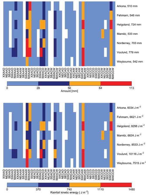
252       A.-M. Tilg et al.: Variation of leading-edge-erosion relevant precipitation parameters   Meteorol. Z. (Contrib. Atm. Sci.)
                                                                                                                           30, 2021

(1 g cm−3 ) is used and for hailstones values between 0.7            many keeping the b-value fixed at 1.50. In contrast to
and 0.9 g m−3 are assumed (Wang, 2013). Rain is the                  Hachani et al. (2017), Kirsch et al. (2019) find higher
dominant precipitation type in the North Sea area, be-               A-values for stratiform rain than for convective rain, but
cause of the temperate climate influenced by the Gulf                a low variability of the b-value for both rain types analy-
Stream. Rain is also assumed to cause most of LEE.                   sing Micro Rain Radar data from North Germany.
Tait et al. (1999) analyse annual and monthly rainfall                   Several studies show that the microphysics of pre-
amount in the North Sea using satellite data and find                cipitation and therefore DSD of rain vary with differ-
that precipitation conditions in the North Sea depend                ent atmospheric conditions (e.g. Hachani et al., 2017).
on land mass distribution but also on general circula-               Hence, there exist a lot of values for A and b for Z-R re-
tion patterns. Furthermore, they show that in some years             lationships, apart from the probably most used A-value
westerlies are less dominant than usual in the North Sea             of 200 and b-value 1.6 attributed to Marshall-Palmer
area and causing a different rain distribution for these             (Ignaccolo and De Michele, 2020). A way to clas-
years. Other precipitation types occur less frequently,              sify different atmospheric conditions is by a weather
but ice and hail can cause severe damage of the lead-                type (WT) or sometimes also called weather pattern.
ing edges during short time (Macdonald et al., 2016;                 Fernandez-Raga et al. (2016) and Fernández-Raga
Letson et al., 2020). Therefore, it is important to con-             et al. (2020) show that westerlies are dominating in
sider the frequency for ice and hail as well. Hail occurs            Spain and that precipitation parameters and soil ero-
frequently in the Midwest of the USA where many wind                 sion patterns vary with WT. Aniol et al. (1980) com-
turbines are in operation (Letson et al., 2020). Compa-              pare Z-R relationships of four different WTs in South
rable observations on hail events in the North Sea area              Germany. They find differences between the A- and
are not available. Punge and Kunz (2016) indicate that               b-values, where the values of the two most frequent WTs
less hail is observed in Europe as compared to the USA.              were quite similar. According to Piotrowicz and Cia-
                                                                     ranek (2020), WT classification is divided into (i) mor-
    The drop-size distribution (DSD) of raindrops is in-
                                                                     phological (defined by daily variation of selected me-
fluenced by the drop formation process and collision
                                                                     teorological parameters) and (ii) genetic (defined by
with other raindrops during their way to the ground.
                                                                     synoptic and atmospheric circulation). Hidalgo and
The number of drops decrease with increasing diam-
                                                                     Jougla (2018) are describing a morphological WT clas-
eter, which is often described with an exponential or
                                                                     sification, but several additional ones are existing. There
gamma distribution. In situ measurements of DSD off-
                                                                     are also several publications describing WTs based on
shore are challenging due to harsh environmental con-
                                                                     genetic aspects like Linderson (2001). Bissolli and
ditions and missing infrastructure. There are only a few
                                                                     Dittmann (2001) define a WT classification for Ger-
measurement campaigns that measured in situ DSD and
                                                                     many also based on synoptic parameters, which should
precipitation type (e.g. Bumke and Seltmann (2012)
                                                                     also be valid for the coastal parts of the North Sea and
and Klepp et al. (2018)). Bumke and Seltmann (2012)
                                                                     Baltic Sea. Hence, we assume that the combination of
compare data from disdrometers installed at research
                                                                     WT and Z-R can give valuable information about DSD
vessels with data from disdrometers installed at land
                                                                     at certain atmospheric conditions.
and find no significant difference in the DSD. The DSD
determines other precipitation parameters like reflectiv-                The aim of this study is to analyse the location- and
ity (Z) and rain rate (R). While Z is proportional to the            weather-type dependence of Z-R relationships, precip-
                                                                     itation types, rainfall amount and rainfall kinetic en-
6th moment of the raindrop diameter and sensitive to
                                                                     ergy using disdrometer measurements at coastal stations
large drops, R is proportional to the 3.67th moment of               of the North Sea and Baltic Sea and the mentioned
the raindrop diameter and more sensitive to drops within             weather-type classification of Bissolli and Dittmann
the 1–3 mm range and the number of drops (Seo et al.,                (2001). We see Z-R relationships as another way to de-
2010).                                                               scribe the DSD for estimating LEE. We assume that
    The Z-R relationship (Z = A ∗ Rb ) describes the em-             the Z-R relationships considering all measurements are
pirical connection between these two precipitation pa-               quite similar for coastal stations at the North Sea and
rameters and is usually applied to convert Z measure-                Baltic Sea, because Bumke and Seltmann (2012)
ments of weather radars into R. Especially the A-value,              found no considerable differences in DSD between land
or prefactor, of the Z-R relationship indicates the pres-            and sea. In contrast, we expect that Z-R relationships of
ence (or absence) of large drops. In case the A-value                specific WTs might vary considerable because of differ-
is in the order of 300, convective rain with large drops             ent atmospheric conditions. Furthermore, we investigate
can be expected. For an A-value around 50, it is driz-               the variance of precipitation type, rainfall amount and
zle (Hachani et al., 2017). According to Doelling                    rainfall kinetic energy for different WTs in the North
et al. (1998), the b-value, or exponent, is of less im-              Sea and Baltic Sea area. Following Tait et al. (1999), we
portance, but also contains some information about                   expect that most precipitation is related to westerlies.
the DSD. Hence, the Z-R relationship is another way to                   The paper is structured as followed: Chapter 2 gives
derive information of the DSD and could be an option                 an overview about the used data. Methods in Chapter 3
for offshore precipitation characterisation. Doelling                include the calculation of the analysed precipitation pa-
et al. (1998) present Z-R relationships for North Ger-               rameters as well as the description of the used weather-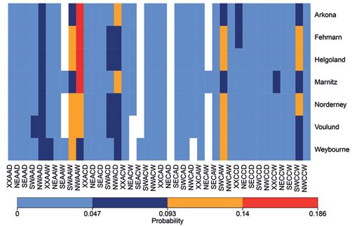
Meteorol. Z. (Contrib. Atm. Sci.)        A.-M. Tilg et al.: Variation of leading-edge-erosion relevant precipitation parameters         253
30, 2021

Figure 1: Map of investigation area including locations of analysed stations. The acronyms used for the stations are explained in the table.

type classification. The results in Chapter 4 present the                  Measurements from 13 different stations in three
location and weather-type dependence of the Z-R rela-                  different countries have been available. All of them are
tionships, precipitation type, rainfall amount and rainfall            at the coast or close to the coast of the North Sea
kinetic energy for the analysed stations. The paper ends               and Baltic Sea where many offshore wind turbines are
with a discussion in Chapter 5 and a conclusion in Chap-               installed (Fig. 1):
ter 6.
                                                                         • Denmark: Data from six Danish stations were pro-
                                                                           vided by Danmarks Tekniske Universitet (DTU) and
2 Data and quality control                                                 Danmarks Meteorologiske Institut (DMI) and in-
                                                                           cluded six datasets measured with Ott in Horns Rev 3
For this study disdrometer measurements were analysed
                                                                           (offshore wind farm), Hvide Sande, Risø, Rødsand
as they measure the number of precipitation particles as
                                                                           (offshore wind farm), Thyborøn, Voulund and one
well as their size and fall velocity. These data also allow
                                                                           dataset measured with Thies in Voulund. In Voulund
the classification of the precipitation particle type and
                                                                           the device was changed from Thies to Ott in 2018.
the calculation of the parameters Z, R, rainfall amount
                                                                         • Germany: Data from six German stations was pro-
and rainfall kinetic energy as they are integral parame-
                                                                           vided on request by Deutscher Wetterdienst (DWD)
ters of the DSD. Data originated from the two disdrom-
                                                                           and included datasets measured with Thies in Arkona,
eter devices Thies Laser Precipitation Monitor (LPM),
                                                                           Bremerhaven, Fehmarn, Helgoland, Marnitz and
henceforward Thies, and Ott Parsivel2 , henceforward                       Norderney.
Ott. Both types generate a horizontal light plane by a                   • United Kingdom (UK): Data measured with Thies in
laser between a transmitter and receiver. The number,
                                                                           Weybourne in the UK was available via the Natu-
size and fall velocity of precipitation particles is deter-                ral Environment Research Council’s Data Repository
mined based on the amplitude and duration of the atten-                    for Atmospheric Science and Earth Observation, also
uation of the laser beam when a particle falls through it.
                                                                           known as CEDA archive (Natural Environment
    However, there are a few differences between the de-                   Research Council et al., 2019).
vices such as the wavelength of the used laser (Thies:
785 nm, Ott: 650 nm) and the housing of the sensors.                       Quality control of the disdrometer data was done
Thies has 22 diameter (0.1875 mm to ≥ 8.000 mm) and                    in three steps. Data were checked related to (i) non-
20 velocity (0.100 m s−1 to 15.000 m s−1 ) classes with                precipitation data by using internal quality parameters,
varying class width and hence 440 classes in total                     (ii) correct precipitation type comparing surface syn-
to refer measured precipitation. Ott has 32 diameter                   optic observation (SYNOP) code from the disdrometer
(0.062 mm to 24.500 mm) and 32 velocity (0.050 m s−1                   with the probability for specific precipitation type using
to 20.800 m s−1 ) classes with varying class width and                 temperature and relative humidity and (iii) limits of size
hence 1024 classes in total. For both devices the mean                 and terminal velocity of raindrops. The necessary tem-
value of the class is given. The performance of both de-               perature and relative humidity data were available via
vices has been focus of several studies (e.g. Frasson                  the Open Data Server from DWD for the German sta-
et al., 2011; Raupach and Berne, 2015; Johannsen                       tions, via CEDA for the UK station (Bandy, 2002) and
et al., 2020). Angulo-Martínez et al. (2018) find that                 on request for Danish stations. Due to high amounts of
Thies measures more small drops while Ott measures                     missing values and data quality issues only the seven sta-
more large drops. According to Fehlmann et al. (2020)                  tions Arkona, Fehmarn, Helgoland, Marnitz, Norderny,
the distinction of rain and snow of Thies is similar to the            Voulund (time series with Thies) and Weybourne were
measurements of the two-dimensional video disdrome-                    used for further analysis. The disdrometer at station Risø
ter (2DVD) (Kruger and Krajewski, 2002)                                was quite sheltered, as the angle between the disdrome-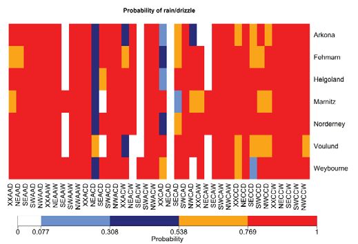
254        A.-M. Tilg et al.: Variation of leading-edge-erosion relevant precipitation parameters           Meteorol. Z. (Contrib. Atm. Sci.)
                                                                                                                                    30, 2021

ter and the surrounding obstacles was equal or above 30°              with Di being the mean drop diameter in class i (mm),
in most directions. Hence, this station was also excluded             N0 as intersect (m−3 mm−1 ), μ as shape factor, and Λ as
from the analysis. For further information about the                  slope (mm−1 ). It is a further quality control step, because
quality control, the reader is referred to the Appendix.              some measured data had no gamma distribution and
                                                                      could not be fitted with this approach, probably because
3 Methods                                                             the measurements did not originate from rain. The rain
                                                                      rate R (mm h−1 ) was then calculated based on Seo et al.
The applied weather-type (WT) classification is based                 (2010):
on Bissolli and Dittmann (2001). The temporal res-
olution of this WT classification is one day, where val-                  R = 6 ∗ π ∗ 10−4 ∗       N(Di ) ∗ D3i ∗ vt ∗ ΔDi (3.3)
ues of an operational weather analysis and forecasting                                              i
system at 12 UTC are used for classification. As this
                                                                      with vt being the terminal fall velocity based on Atlas
WT classification was developed with focus on Ger-
many, DWD provides the time series of WTs back to                     et al. (1973) (m s−1 ) and ΔDi being the diameter inter-
1979 free of charge on its website. In this study, we used            val (mm). The terminal fall velocity based on Atlas
this free available time series of WTs of DWD.                        et al. (1973) is calculated as follows:
    Bissolli and Dittmann (2001) use five letters to                                    vt = 9.65 − 103 ∗ e−600∗Di                     (3.4)
describe the WT and the related atmospheric conditions.
The first two letters describe the advection direction                The reflectivity Z (mm6 mm−3 ) was calculated as fol-
(horizontal wind direction in 700 hPa), the following                 lows (Seo et al., 2010):
two letters describe the cyclonality in 950 and 500 hPa
and the last letter the humidity (precipitable water in the                           Z=       N(Di ) ∗ D6i ∗ ΔDi     (3.5)
troposphere above or below to the long-term mean of                                            i
1979 to 1996). There are following options for each of
the letters:                                                          To determine the A- and b-value of the Z-R relationship,
                                                                      a nonlinear least-squares estimate with Z as independent
 • Advection: NE (northeast), SE (southeast), SW                      variable of the following nonlinear model, derived from
   (southwest), NW (northwest), XX (no prevailing                     equation (3.1), was performed:
   wind direction in case less than two thirds of the grid
                                                                                                        ∗   log(Z)−A∗ )
   points have wind from the same direction)                                                 R = 10(b                                  (3.6)
 • Cyclonality: anticyclonic (A; large-scale circulation
   in clockwise direction), cyclonic (C; large-scale cir-             This was done using R 4.0.1 (R Core Team, 2020) and
   culation in anti-clockwise direction)                              the function nls in the stats package. According to Kra-
 • Humidity: wet (W), dry (D)                                         jewski and Smith (1991) and Alfieri et al. (2010) a
                                                                      linear regression estimation using the log-scale of R and
    All possible combinations lead to a total number of               Z would lead to biased values of the A- and b-value.
40 weather types (WTs). For example, the WT with                      For each station a Z-R relationship was fitted using all
the abbreviation NWAAW describes an advection from                    1-minute measurements, independent of the WT clas-
northwest (NW), the cyclonality in 950 and 500 hPa is                 sification or event. Furthermore, separate Z-R relation-
anticyclonic (AA) and a wet atmosphere (W). The WT                    ships were fitted using only Z and R values related to
with the abbreviation SECAW describes an advection                    the specific WT. To calculate the Root Mean Square Er-
from southeast (SE), the cyclonality in 950 hPa is cy-                ror (RMSE) between measured R and R based on the
clonic (C), the cyclonality in 500 hPa is anticyclonic (A)            fitted Z-R relationship, 75 % of the data were used for
and a wet atmosphere (W).                                             fitting the A- and b-value, the remaining 25 % for an in-
    Quality controlled disdrometer data with a temporal               dependent calculation of the error (training and valida-
resolution of 1 minute were used to calculate LEE rele-               tion dataset). Only measurements with R > 0.1 mm h−1
vant precipitation parameters.                                        were considered in the training process. The choice of
    The relationship between Z and R is usually de-                   this R threshold influences the fitted A- and b-values as
scribed with a power law:                                             well (Verrier et al., 2013). If the number of training val-
                         Z = A ∗ Rb                         (3.1)     ues was below 50, no fitting was done. Therefore, not all
                                                                      stations had Z-R relationships for all WTs. The RMSE
with A as the prefactor and b as the exponent. Both,                  is defined as:
Z and R, depend on the DSD, often described with a
                                                                                                1
drop concentration N(Di ) (m−3 mm−1 ). For this study                                 RMSE =             (yi − oi )2        (3.7)
N(Di ) was calculated using the parameterization ap-                                            n      i
proach from Ulbrich and Atlas (1998) considering
only rain, where                                                      where y is the calculated R, o the measured R and n the
                                    μ                                 number of pairs. For the calculation of the RMSE it
                N(Di ) = N0 ∗ Di ∗ e−ΛDi                    (3.2)     was assumed that the measured R was the calculated R
Meteorol. Z. (Contrib. Atm. Sci.)         A.-M. Tilg et al.: Variation of leading-edge-erosion relevant precipitation parameters          255
30, 2021

Figure 2: Fitted A- and b-values of the Z-R relationship for all stations. The points represent A and b fitted using all 1-minute measurements.
The bars indicate the range of A and b fitted with measurements taken during specific weather types.

based on the parameterized DSD calculated with equa-                     mean annual KE, the same procedure was applied as for
tion (3.3).                                                              the mean annual rainfall amount.
    Rainfall amount (AMT; mm) is the volume of all                          A probability was calculated to investigate the fre-
measured raindrops and was calculated using disdrome-                    quency that for a certain WT precipitation was registered
ter data and following equation:                                         or a certain precipitation type occurred:
                       1 π                                                        #measurements fulfilling requirements
               AMT = ∗ ∗           ni ∗ D3i      (3.8)                       P=                                                        (3.10)
                       A 6       i
                                                                                            #measurements

where A is the measuring area (m2 ) and ni the num-                      4 Results
ber of drops. To get a mean annual rainfall amount for
each station although having incomplete years, follow-                   4.1 Z-R relationship
ing procedure was applied: (i) Sum of rainfall amount
over whole available time period, (ii) Number of days                    The A- and b-values of the location-specific Z-R rela-
between first and last observation, (iii) Division of over-              tionship were fitted using quality controlled 1-minute
all rainfall amount by number of observation days and                    disdrometer data and considering only rain. To evalu-
multiplication of this value with 365 to get mean an-                    ate the dependence on WTs, separate A- and b-values
nual rainfall amount. The annual mean value should not                   were fitted using only data measured during the spe-
be influenced that much by gaps, because only stations                   cific WT. Fig. 2 shows the distribution of the fitted A-
with a low amount of missing values were selected.                       and b-values for each location. The points represent the
    Rainfall kinetic energy per area (KE, J m−2 ) is based               A- and b-values based on all measurements indepen-
on Petrů and Kalibová (2018):                                           dent of the WT. The A-values vary between 164 (Mar-
                   1 ρ ∗π
                                                                         nitz) and 233 (Weybourne). The higher (lower) A-value
             KE =                 ni j ∗ D3i ∗ v2j    (3.9)              might be due to slightly larger (smaller) mean drop
                   A 12 i j                                              diameters at Weybourne (Marnitz). The b-values var-
                                                                         ied between 1.74 (Helgoland) and 1.88 (Voulund) and
where ρ is the water density (kg m−3 ). For this study the               were quite similar. The horizontal and vertical bars indi-
fall velocity of the raindrops measured by the disdrom-                  cate the range of A- and b-values of the analysed WTs.
eter was used for the KE calculation. Hence, only the                    The station Weybourne had the largest spread of A-
KE provided by rainfall was analysed. To calculate the                   and b-values with A-values between 21 and 699 and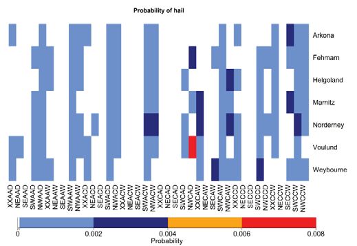
256          A.-M. Tilg et al.: Variation of leading-edge-erosion relevant precipitation parameters        Meteorol. Z. (Contrib. Atm. Sci.)
                                                                                                                                   30, 2021

Figure 3: Weather-type (WT) dependence of (a) A-values and (b) b-values. Box-whiskers plots show the variability of the values for
each WT. The box is represented by the 1st and 3rd quartile and the whiskers by 1.5 times the interquartile range above and below the 1st and
3rd quartile. Values above or below the whiskers are outliers. The coloured points represent the value of the specific station. The WT is
described with five letters, where the first two letters describe the advection direction (NE, NW, SE, SW, XX = no prevailing direction),
the following two letters describe the cyclonality in 950 and 500 hPa (A(nticyclonic), C(yclonic)) and the last letter the humidity index
(W(et), D(ry)).

b-values between 1.21 and 3.05. The bars of the re-                     quartile and with the thick line being the median. The
maining stations cover a similar range of values. The                   whiskers are 1.5 times the interquartile range (IQR)
A- and b-values of station Fehmarn for WT NEAAD                         above the third quartile and below the first quartile,
were not considered in Fig. 2 and Fig. 3, because the                   where the interquartile range is the difference between
A-value with 2997 and the b-value with 3.15 were much                   the third and first quartile. Values above or below the
higher compared to the other fitted values. These high                  whiskers are classified as outliers. That means that a
values might be caused by the fact that only R values                   small box and short whiskers indicate a small variability
below 1 mm h−1 were measured during this WT. All fit-                   of the values, while a large box and large whiskers in-
ted A- and b-values can be found in the Appendix.                       dicate a large variability. The box-whiskers plots were
    The WT-dependence of A and b at the different lo-                   overlaid with the WT-specific A- and b-values of the
cations is investigated more deeply next. Fig. 3 shows a                stations. For five WTs (SEACD, NEACW, SEACW,
box-whiskers plot of the A- and b-values for each WT.                   NECAD, NECAW) no station had the required number
The box represent the values within the first and third                 of 50 measurements to fit the Z-R relationship. For three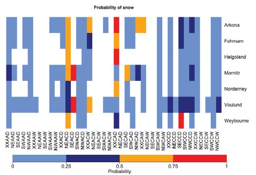
Meteorol. Z. (Contrib. Atm. Sci.)       A.-M. Tilg et al.: Variation of leading-edge-erosion relevant precipitation parameters      257
30, 2021


Figure 4: Mean 1-minute parameterized drop concentration for the weather types (left) NWAAW (advection from Northwest, anticyclonality
in 950 and 500 hPa, wet humidity index) and (right) SECCD (advection from Southeast, cyclonality in 950 and 500 hPa, dry humidity index).
The number of considered 1-minute values is given in the parenthesis next to the station name.

WTs (SEAAD, SEAAW and SECAD) it was only sta-                         gated further in the next chapter. To summarize, the A-
tion Weybourne that had enough measurements to fit the                and b-values varied to a certain degree between the loca-
A- and b-values of the Z-R relationship.                              tions for all WTs, where only for a few WTs the values
    For 28 out of 32 WTs the median of the A-values                   varied considerable between different locations.
had a value of 200 +/− 50. Two WTs (NEAAW and                             The variability of A- and b-values can be compared
XXCAW) had a median below 150 and two WTs                             with the variability of the mean DSD, as Z and R de-
(XXACW and SECCD) had a median above 250. Higher                      pend on the DSD. As an example, Fig. 4 shows the mean
(lower) A-values indicate that a higher (lower) amount                1-minute parameterized DSD of the WTs NWAAW and
of large raindrops was observed during these WTs,                     SECCD. The parameterization of the DSD was done
maybe related to more (less) convective rain. Although                following the steps described in Ulbrich and Atlas
the similar median values support a small variability be-             (1998). While the WT NWAAW had a low variability
tween WTs, the difference between the highest and low-                of A- and b-values between the stations, SECCD had
est A-value of each WT showed a large variability be-                 one of the largest variabilities of A- and b-values. The
tween the stations for some specific WTs. While 11 out                drop concentrations in Fig. 4 showed a similar pattern.
of 32 WTs had a maximum-to-minimum difference be-                     For the WT NWAAW the difference between the drop
low 100, four WTs (NEAAD, NEACD, NECCD and                            concentrations of the stations was small. In contrast, for
SECCD) had a difference above 500. These high vari-                   the WT SECCD there were quite some differences be-
ations would lead to the assumption that the underlying               tween the drop concentrations at all diameters. The num-
DSD of the stations was quite different for the same WT.              ber of 1-minute observations available to calculate the
    The majority of the median b-values were within                   A- and b-values were much higher for the WT NWAAW
1.90 +/− 0.30. One WT (NWCAD) had a median b-value                    (min. 4152) compared to WT SECCD (max. 496).
above 2.20, while one WT (NECCW) had a median                             A performance indication of the fitted A- and
b-value below 1.70. Equal to the A-value, the maximum-                b-values is the error between measured and calculated R.
to-minimum difference of the b-values of the stations                 In Fig. 5 the distribution of the Root Mean Square Er-
was quite high for some WTs. The difference included                  ror (RMSE) between the measured R and the calculated
values between 0.20 for WT SWCCW and 1.86 for WT                      R for all WTs is shown using box-whiskers plots. The
NEAAD.                                                                RMSE was calculated for each station and WT using
    A comparison of WTs with a high variation for dif-                the validation dataset. The fitted A- and b-values and
ferent locations showed that they (i) often had a high                the A- and b- value based on Marshall-Palmer, respec-
variability of A- and b-value (e.g. WTs NEAAD or                      tively, were used to calculate R. The applied Marshall-
SECCD) and (ii) were often fitted with the minimal                    Palmer values were: A = 200, b = 1.6 (Marshall et al.,
number of 50 observations or only slightly more. The                  1955). The median of the RMSE values, indicated by
low number of observations leads to the assumption that               the black thick line in Fig. 5, was lower for R us-
the specific WT occurred rarely. This will be investi-                ing WT dependent A- and b-values compared to the R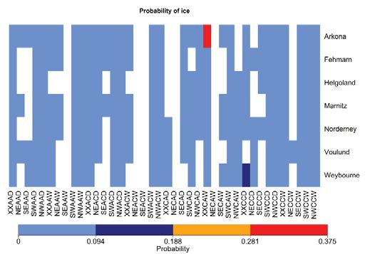
258         A.-M. Tilg et al.: Variation of leading-edge-erosion relevant precipitation parameters        Meteorol. Z. (Contrib. Atm. Sci.)
                                                                                                                                  30, 2021

Figure 5: Distribution of the Root Mean Square Error (RMSE) between measured rain rate and calculated rain rate for 40 weather
types (WT). For the orange boxplots WT-dependent A- and b-values were used. For the blue boxplots the values A = 200 and b = 1.6
based on Marshall-Palmer were used. Black dots are the RMSE values of the different WTs.

using Marshall-Palmer. The median RMSE varied be-
tween 0.64 (Marnitz) and 1.06 (Helgoland) using the fit-
ted A- and b-values and between 0.71 (Fehmarn) and
1.27 (Helgoland) using Marshall et al. (1955). Over-
all, the lower error for R calculated with WT-dependent
A- and b-values indicates a higher accuracy compared
to R values calculated with a standard Z-R relationship.

4.2 Dependence of precipitation probability
    on weather type
To find WTs with the highest precipitation probabil-
ity considering all precipitation types, for each station
the cumulative number of minutes with precipitation
was related to the cumulative number of minutes with                   Figure 6: Probability to observe precipitation and its dependence
precipitation for a specific WT (Fig. 6). It was found                 on the weather type. Probabilities above zero are represented by the
                                                                       given colour scale. White areas represent a probability of zero.
that only two WTs (SWAAW, NWAAW) had probabil-
ities above 0.14 to observe precipitation. For another
three WTs (NWACD, SWCAW and SWCCW) the prob-
ability was between 0.093 and 0.14. The probability to                 4.3 Distribution and weather-type dependence
observe precipitation of any kind in one of these five                     of precipitation types
WTs was between 0.44 (Weybourne) and 0.56 (Hel-
goland). For comparison, WTs with a large spread of                    As mentioned, occurrence of hail (and ice) can be harm-
fitted A- and b-values of the Z-R relationship (e.g.                   ful for LEE. Therefore, it is necessary to investigate the
NEAAD and SECCD) had a probability below 0.01.                         distribution of different precipitation types on the overall
Low probabilities or a complete absence of precipitation               time with precipitation. Table 1 gives an overview of the
was observed for five WTs (SEAAW, NEACW, SEACW                         cumulative number of minutes with precipitation, which
and NWCAD, NECAW). For one WT (NECAD) no                               depends on the length of the available time series, and its
station observed any precipitation during the analysed                 distribution over the five different precipitation groups.
time period. This analysis shows that precipitation ob-                The precipitation type rain was observed most often with
servations were dominated by WTs with SW and NW                        a percentage between 90.03 % (Arkona) and 95.89 %
advection.                                                             (Helgoland). The precipitation type snow was observed
Meteorol. Z. (Contrib. Atm. Sci.) A.-M. Tilg et al.: Variation of leading-edge-erosion relevant precipitation parameters 259
30, 2021
Table 1: Minutes with precipitation and distribution over the five defined precipitation groups.
Station # Minutes with precipitation % Rain/drizzle % Mixed rain/snow % Snow % Ice % Hail
Arkona 218984 90.03 1.07 8.57 0.30 0.03
Fehmarn 232254 92.40 1.13 6.16 0.26 0.05
Helgoland 188579 95.89 1.13 2.22 0.69 0.07
Marnitz 225075 90.50 1.31 7.68 0.48 0.03
Norderney 250887 94.77 0.90 2.62 1.60 0.11
Voulund 412218 91.11 0.95 7.41 0.47 0.06
Weybourne 127603 95.83 0.38 2.45 1.29 0.05
second most and between 8.57 % (Arkona) and 2.22 % The probability to observe precipitation in form of
(Helgoland) of the analysed precipitation time. Except ice was except for the station Arkona (WT XXACW)
for Norderney, these two precipitation types were ob- below 0.147 (centre right in Fig. 7). The probability
served in more than 98 % of the time with precipitation. of 0.375 at station Arkona for the mentioned WT was
The remaining precipitation types, mixed (rain and snow caused by the ratio of 8 minutes precipitation to 3 min-
at the same time), ice and hail occurred between 1.60 % utes with ice.
(Norderney, ice) and 0.03 % (Arkona, hail) of the time. According to the bottom plot in Fig. 7, the probability
The stations Norderney and Weybourne had in compari- to observe hail was below 0.004 except for the station
son to the other stations a high percentage of the precip- Voulund (WT NWCAD). The probability of 0.008 at
itation type ice. Voulund was caused by the relation of 7 minutes with
To investigate the dependence of the precipitation hail to 856 minutes with precipitation in total.
type on the WT, the probability between the number of It is important to note that the number of ice and
minutes with precipitation for one specific WT and the hail observations were low, especially for rare WTs.
number of minutes with a specific precipitation type for This factor must be considered when interpreting the
one specific WT was calculated. Fig. 7 shows the proba- probability values.
bility to observe a specific precipitation type depending
on the WT.
For the precipitation types mixed, ice and hail sin- 4.4 Weather-type dependence of annual
gle high probabilities compared to rain and snow were
observed. For the precipitation types rain, snow and hail rainfall amount and rainfall kinetic energy
some dependence on the WT can be seen in Fig. 7. Some
WTs with advection from east and no prevailing advec- For a siting assessment of wind turbines related to LEE,
tion direction, respectively, had a lower probability of not only information of the DSD might be relevant but
rain but a higher probability of snow. The precipitation also cumulative values of rainfall amount or rainfall ki-
type hail occurred mostly related to WT with advection netic energy (KE). Fig. 8 shows the mean annual rainfall
from NW or SW. amount and KE per WT. Only rain was considered for
As already shown in Table 1, the probabilities to both parameters and KE was calculated using the mea-
measure rain or snow were highest. Hence, it is not sured fall velocity of the raindrops. As the analysed time
surprising that most WTs had the highest probability to series had a different length, a mean daily value was cal-
observe rain. Apart from 0, the lowest probability was culated and multiplied with 365 to get the mean annual
0.077 (Marnitz, SEACD) and multiple stations and WTs rainfall amount and KE, respectively.
had a probability of 1. A probability of 1 means in this The mean annual values were higher at stations close
connection that precipitation occurred only as rain and the eastern part of the North Sea (Helgoland, Norderney
no other precipitation type was observed during this WT. and Voulund) with values above 700 mm / 8500 J m−2 . In
As the top right plot in Fig. 7 shows, for two WTs contrast, stations at or close to the Baltic Sea or the west-
(NEACD, XXCAD) half or more of the stations had a ern part of the North Sea (Arkona, Fehmarn, Marnitz
probability higher than 0.5 to observe snow. This high and Weybourne) had values below 550 mm / 7500 J m−2 .
probability means that in case this WT was observed Interestingly, Weybourne had a higher KE although hav-
during half of the time or more the registered precipi- ing a similar rainfall amount as the other stations. This
tation type was snow. For the WT SEACD the station example shows that the ratio between rainfall amount
Voulund had even a probability of 1 to observe snow. and KE was not the same for all stations. The difference
In case of the precipitation type mixed (centre left is caused by a higher number of larger raindrops (with
in Fig. 7), the station Helgoland is outstanding. In this higher fall velocity) in Weybourne as already indicated
case, 19 out of 60 minutes with precipitation during WT by the higher fitted A-value in Section 4.1.
SEACD were classified as mixed and led to a probability The absolute rainfall amount per WT varied between
of 0.317. The remaining probabilities to observe mixed the lower threshold of 0.01 mm and 113 mm (Voulund,
were below 0.115. SWAAW). Five WTs (SWAAW, NWAAW, SWACD,260 A.-M. Tilg et al.: Variation of leading-edge-erosion relevant precipitation parameters Meteorol. Z. (Contrib. Atm. Sci.)
30, 2021
Figure 7: Probability to observe (top left) rain/drizzle, (top right) snow, (centre left) mixed, (centre right) ice and (bottom left) hail depending
on the weather type. Probabilities above zero are represented by the given colour scale. White areas represent a probability of zero.
SWCAW and SWCCW) registered rainfall amounts contributed between 40 (Arkona) and 53 % (Weybourne)
above 84 mm. Furthermore, these five WTs provided to- to the overall KE per station. For six WTs (SEAAD,
gether between 50 (Marnitz) and 58 % (Voulund) of the SEAAW, NEACW, SEACW, NECAD, NECAW) the
annual rainfall amount at all stations. These WTs were majority or all of the stations registered no or negligi-
also WTs with the highest probability to be observed bly rainfall amount and KE, respectively. Hence, both
(see Fig. 6). The pattern is similar for KE, where val- parameters were dominated by rain related to advec-
ues up to 1480 J m−2 (Voulund, SWAAW) were calcu- tion from Southwest (SW). Furthermore, the compari-
lated for a single WT. Four WTs (SWAAW, SWACD, son shows that a similar rainfall amount can lead to dif-
SWCAW, SWCCW) had values above 1110 J m−2 and ferent values of KE.Meteorol. Z. (Contrib. Atm. Sci.) A.-M. Tilg et al.: Variation of leading-edge-erosion relevant precipitation parameters 261
30, 2021
cipitation parameters like rain rate. As the real ground
truth of precipitation is not known, it is difficult to quan-
tify the uncertainty of both sensors in absolute numbers.
Raupach and Berne (2015) propose an algorithm to
correct the measured drop fall velocity of an Ott using
data of a two-dimensional video disdrometer (2DVD).
According to them, this correction algorithm is appli-
cable to different disdrometer types and locations and
increases the accuracy of DSD-based precipitation pa-
rameters. Adirosi et al. (2018) conclude that for estab-
lishing long-term radar algorithms the disdrometer type
plays a smaller role than for analysing the microphysics
of a single event. As the focus of the above presented re-
sults was on long-term values, their conclusion are pos-
itive news for this study.
Despite the applied quality control of the disdrom-
eter data, it was not possible to avoid having non-
precipitation particles in the applied DSD. In case of the
Z-R fitting procedure, the parameterisation of the DSD
for calculating rain rate and reflectivity, worked as addi-
tional quality control step. In case of the quality control
of the precipitation type only the plausibility of observ-
ing a specific type was investigated, but not the plausi-
bility of precipitation itself. The latter would have only
been possible using data from other sensors, which were
not available for all stations. Such non-precipitation par-
ticles can led to some unrealistic results. An additional
problem related to the precipitation type is that Thies
Figure 8: Mean annual (top) rainfall amount and (bottom) rain-
and Ott store only the highest WMO SYNOP value,
fall kinetic energy (KE) registered per weather type. Values above
0.01 mm / 0.01 J m−2 are represented by the given colour scale.
although different WMO SYNOP values and therefore
White areas represent no rainfall amount / KE or values below the precipitation types can occur at the same time (e.g. rain
threshold. The mean cumulative value for each station is given next and hail during a thunderstorm). Furthermore, precipita-
to the station name. tion type statistics from disdrometers give only a very
local impression especially in relation to ice or hail.
In general, events with hail are not frequent and often
5 Discussion only local. Hence, it is not very likely to observe hail
within the small measurement area of the disdrometer
(0.0054 m2 for Ott and 0.00456 m2 for Thies). To con-
The erosion of the leading edges of wind turbine blades firm such results, observations should be validated with
is caused by the impact of hydrometeors. To estimate human observers or data from dual-polarization weather
spatial variations of precipitation parameters relevant radars.
for LEE, several parameters like Z-R relationship, pre- Not only non-precipitation particles in the dataset,
cipitation type, rainfall amount and rainfall kinetic en- but also the duration of the time series, the related fre-
ergy were analysed regarding their variation with loca- quency of specific WT and occurrence of extreme values
tion and weather type (WT). We showed that the Z-R (low or high) can lead to uncertainties in the results. For
relationship of seven analysed stations was similar but example, in case of the station Fehmarn a lot of low R
varied considerable for some WTs. WTs with advection values were measured during a WT with low probability
from NW and SW were most dominant and provided (NEAAD) and caused A- and b-values varying strongly
the majority of annual rainfall amount and rainfall ki- from the other values. Doelling et al. (1998) mention
netic energy. Rain and snow were observed around 98 % that small samples can produce a statistical variability
of the time, precipitation in form of ice and hail during that could be wrongly interpreted as natural variability.
the rest of the time. Hence, one needs to be cautious in analysing and inter-
All shown results were based on measurements preting data from infrequent WT and precipitation types.
with the disdrometers Thies LPM and Ott Parsivel2 . According to Krajewski and Smith (1991) more than
Angulo-Martínez et al. (2018) report that the Thies 10000 independent data samples are required to get valid
measures more small raindrops than Ott, while Ott tends estimates of A- and b-values. However, as the time pe-
to underestimate the fall velocity compared to a theoret- riods of the analysed disdrometer measurements were
ical fall velocity model and Thies. They show that this short from a climatological aspect, this requested num-
behaviour has implications for all DSD-dependent pre- ber of data samples could not be fulfilled in this investi-262 A.-M. Tilg et al.: Variation of leading-edge-erosion relevant precipitation parameters Meteorol. Z. (Contrib. Atm. Sci.)
30, 2021
gation. The low number of observations influenced also lower percentages for stations at the North Sea coast.
the probability of observing a specific precipitation type. The dominance of rain is not surprising as temperature
For example, high probabilities of ice or hail calculated is mostly above freezing level. Lower temperatures at
for rare WTs must be interpreted with caution and might stations inland and continental influence related to ad-
not always reflect the climatological conditions. vection from the east cause higher snow fractions for
A drawback from the applied weather-type classifi- stations inland and at the coast of the Baltic Sea. Ice and
cation is that the WT is assigned every day at 12 UTC. It hail are not so frequent as atmospheric conditions usu-
can happen that the synoptic conditions changed before ally do not favour the formation of it (e.g. Punge and
or after that time and would require allocating measured Kunz (2016)). Licznar and Krajewski (2016) find a
precipitation to another WT. similar fraction of mixed and hail analysing data from
The range of fitted A-values of all stations var- an Ott in Warsaw. However, it is unclear to which ex-
ied between 164 and 233 using all 1-minute measure- tend hail and ice particles were recorded correctly by
ments independent of the WT and was therefore around the disdrometers. Pickering et al. (2019) mention some
the frequently used A-value of 200 (Marshall et al., difficulties of the Thies to classify graupel.
1955). The fitted b-values (1.74–1.88) are slightly above The annual rainfall amount and rainfall kinetic en-
the frequently used b-value of 1.6 (Marshall et al., ergy (KE) had higher values in the eastern part of the
1955). While Marshall and Palmer (1948) publish an North Sea compared to lower values in the western part
A-value of 220 and a b-value of 1.60, Marshall et al. of the North Sea and the Baltic Sea. The increase of
(1955) mention revised values of A = 200 and b = 1.6 for rainfall amount from west to east across the North Sea
the Z-R relationship. The low variation between the dif- is already mentioned by Tait et al. (1999) who analyse
ferent locations follows the assumption based on Bumke satellite rainfall data. The absolute values of the rainfall
and Seltmann (2012) who state a low variation of DSD amount of the stations in Germany are in accordance
between sea and land considering data from the North with reported values of around 700 to 800 mm on the
Sea and Baltic Sea. coast of the North Sea and 550 to 600 mm on the coast
The dependence of fitted A- and b-values on the WT of the Baltic Sea (Deutscher Wetterdienst, 2020).
was less pronounced as expected, especially the me- Davison et al. (2005) estimate the monthly KE based
dian values of A and b were within the same range. on average daily rainfall data in England and Wales and
WTs with a lot of observations had a smaller difference find values between 375 and 625 J m−2 for the area of
between highest and lowest A- and b-value compared Weybourne. These values give an annual value up to
to WTs with a low number of observations. However, 7500 J m−2 , which is comparable to the calculated value
for some of these rare WTs only low R were measured, in this study.
which indicates some kind of dependence on the WT. However, one could argue that the calculated KE is
Aniol et al. (1980) also find a WT-dependence of the not the kinetic energy of drops that impact the turbine
A- and b-values analysing measurements in South Ger- blade as only the measured fall velocity was used to cal-
many. Similar to this study the A- and b-values of fre- culate that. One of the challenges with calculating the
quent WTs have a small difference. It is interesting to actual impact velocity of the drops is that this velocity
note that their weighted mean A-value is higher (256) depends on the tip speed of the wind turbine which itself
and b-value is lower (1.42), respectively, compared to is a factor of the wind speed and the wind turbine type
the values of this study. This indicates that in South Ger- (Hasager et al., 2020). To calculate the impact veloc-
many more large drops are measured. This is not sur- ity, the wind speed at hub-height and turbine operation
prising, because already Bringi et al. (2003) have shown including rotational speed and blade length are needed.
that the mass-weighted mean drop size is larger for con- Typical meteorological wind speed measurements on the
tinental locations than for maritime locations. Hachani ground do not represent correctly the wind speed at the
et al. (2017) find no strong dependence of the Z-R rela- turbine height as wind speed increases with increasing
tionship on specific WTs, but on the rainfall types like distance from the surface. At offshore locations, in situ
stratiform and convective. This is supported by Kirsch meteorological data are not easy available. Letson et al.
et al. (2019) and other studies that show a clear differ- (2020) use wind speed from radars. Alternatively, mod-
ence of the A- and b-values for convective and strati- elled winds could be used for the offshore environment.
form rain. Frequent WTs might experience both, con- In situ precipitation measurements with disdrometers
vective as well as stratiform rain, and the resulting A- are challenging offshore as there is hardly no infrastruc-
and b-values represent an average condition. These rela- ture to install sensors and wind affects the registration
tions indicate that probably no rain type is dominant for of the particles. Regarding the latter, disdrometers can
frequent WTs but for rare WTs. However, based on the be optimized for these harsh conditions, for example
results in this study it is not completely clear if the high by using an articulating disdrometer (Friedrich et al.,
(low) variability of some WTs is related to a low (high) 2013a) or a disdrometer with a cylindrical measurement
number of observations or caused by different (same) volume (Klepp, 2015). Ideally though would be to com-
and re-emerging DSD at the stations. bine blade speed from wind farm operation with the Z-R
For all stations rain occurred in more than 90 % of based KE information at wind farm sites to assess and
the time, the percentage of snow was quite variable with predict LEE.Meteorol. Z. (Contrib. Atm. Sci.) A.-M. Tilg et al.: Variation of leading-edge-erosion relevant precipitation parameters 263
30, 2021
In general, by disregarding all precipitation types ex- of snow was an exception as its probability was domi-
cept rain for calculating the rainfall amount and the rain- nated by WTs with advection from the east and no pre-
fall kinetic energy, both values might be slightly under- vailing advection. Annual values of rainfall amount and
estimated as rain of events with mixed precipitation is rainfall kinetic energy were higher for stations at the east
missing. coast of the North Sea and lower for stations close to the
WTs with advection from NW and SW were dom- Baltic Sea and the west coast of the North Sea.
inating the precipitation probability as well as the an- Assuming that the risk of erosion of the leading edges
nual rainfall amount and annual KE. That is not sur- is governed by the cumulative rainfall amount or rainfall
prising as the weather is dominated by westerlies (Tait kinetic energy, wind farms in the eastern part of the
et al., 1999). Fernandez-Raga et al. (2016) and Fer- North Sea have a higher risk than in the western part
nández-Raga et al. (2020) also find high rain values or in the Baltic Sea. As the number of large drops might
for westerly directions in Spain. It is still part of ongo- also play a role in the development of LEE, the western
ing research activities to investigate whether the annual part of the North Sea might also have a higher risk,
rainfall amount, events with high rain rates or other rain- because Weybourne had higher A-values for the Z-R
fall parameters describe the influence of rain on LEE relationship.
best. Assuming that the annual rainfall amount is the The demand of precipitation measurements offshore
dominant criterion for LEE, than the most frequent WTs will increase, because more wind farms will be in-
cause most damage. However, Hasager et al. (2020) stalled in the North Sea and Baltic Sea and an estimation
stated that not only rain but also the wind climate has of LEE risk probably gets more important. As in situ
an influence on the development of LEE. Therefore, fur- measurements are challenging due to frequently miss-
ther analyses are needed to find out which WT causes ing infrastructure, LEE relevant precipitation parameters
most LEE. could be calculated using Z-R relationships and annual
values to estimate drop size and frequency of drop sizes.
6 Conclusion Acknowledgements
The impact of precipitation particles cause degradation We would like to thank DMI, DWD (P. Tracksdorf),
of the leading edge of wind turbine blades, better known NERC (B. Pickering) and UEA (G. Forster) for pro-
as leading-edge erosion (LEE). To understand the role viding data. The main author likes to thank the ERO-
of precipitation on LEE better, we investigated the vari- SION project funded by the Innovation Fund Denmark
ation of relevant precipitation parameters with location grant 6154-00018B and DTU for funding. Furthermore,
and weather types (WTs). The focus was on analysing we are grateful to the comments of two anonymous re-
Z-R relationships and precipitation type as well as on an- viewers.
nual rainfall amount and annual rainfall kinetic energy.
As LEE seems to be more severe offshore, we chose 7 Appendix 1
the area of the North Sea and Baltic Sea with several
wind farms installed as investigation area. As there are 7.1 Quality control based on internal
only limited offshore in situ precipitation measurements disdrometer data
available, we focused on data from coastal stations.
We found that the variations of the A- and b-values All disdrometer data from the above mentioned stations
of the Z-R relationship using all 1-minute measurements undergone the steps listed in Table 2 to ensure that all
varied only slightly between the stations. This result non-precipitation related particles were filtered out.
supports our hypothesis that the mean microphysics and Table 3 gives an overview about start and end date of
therefore drop-size distributions (DSD) at the stations the available time series, the disdrometer type, number
are quite similar. The Z-R relationships fitted for spe- of 1-minute intervals, percentage of missing 1-minute
cific WTs varied notable for some WTs. It is not clear intervals as well as percentage of intervals that were dis-
if the WT or the low number of measurements for fit- regarded by the quality control steps described in Ta-
ting the A- and b-value causes this higher variability. ble 2. No measurements were disregarded applying cri-
Hence, further research is needed on that. Furthermore, teria QC1-7 and QC1-10 and therefore are not listed in
we showed that using WT-dependent Z-R relationships Table 3. The percentage of missing values was above
improve the estimation of R based on Z compared us- 20 % for the stations Bremerhaven, Horns Rev3, Hvide
ing the Marshall-Palmer values. The most frequent mea- Sande, Thyborøn and Voulund. Additionally, the sta-
sured precipitation type was rain and drizzle, followed tions Horns Rev 3, Hvide Sande, Rodsand and Thyborøn
by snow. Other precipitation types like ice and hail were showed a high percentage of measurements with a status
measured only for a few minutes each year. Our hypoth- problem and/or low laser amplitude. These four stations
esis was proved that the highest precipitation probability are located at offshore wind farms (Horns Rev 3, Rød-
is associated to WTs with advection from NW or SW sand) and at the west coast of Denmark (Hvide Sande,
due the dominance of westerlies. The WT-dependence Thyborøn), respectively. The occurring harsh conditions264 A.-M. Tilg et al.: Variation of leading-edge-erosion relevant precipitation parameters Meteorol. Z. (Contrib. Atm. Sci.)
30, 2021
Table 2: Quality control of disdrometer data based on internal measured values of the disdrometers Thies LPM and Ott Parsivel2
Step Argument Description
QC1-1 Status Status is different for Thies and Ott
Ott has a parameter called “status”. Only measurements with status
0 and 1 were accepted.
Status of Thies was defined as a combination of laser and heating
parameters (columns 116 to 144 in Telegram 5 according to manual
of version 5.4110.xx.x00). If one of the parameters indicated an
error, the measurement was disregarded.
Special case station Weybourne: A Thies was installed, but the data
provider introduced its own definition of data quality. Only data with
quality flag equal to 1 was accepted.
QC1-2 Cumulative number of observed particles < 10 Measurements with less than 10 particles in 1 min were disregarded.
Reference: Tokay and Bashor (2010)
QC1-3 Rain rate < 0.01 mm h−1 Measurements with less than 0.01 mm h−1 in 1 min were
disregarded. Reference: Tokay and Bashor (2010)
QC1-4 Data in less than 5 size-velocity combinations Inspired by Ghada et al. (2018)
QC1-5 Negative SYNOP code According to the Thies manual a negative SYNOP 4680 code
indicates a sensor error. Such data was disregarded.
QC1-6 SYNOP code indicates unknown precipitation (41, 42) According to the Thies manual, SYNOP 4680 code 41 and 42
characterize unknown precipitation and it is recommended not to use
this data. Such data were disregarded.
QC1-7 Low measurement quality Thies has a parameter called “measurement quality”. Only data
> 0 % to 100 % was accepted.
QC1-8 Sample interval is not 60 s Ott has a parameter called sample interval due to use of DTU
internal data collection software. Only data with a sample interval
of 60 s (= 1 min) was accepted.
QC1-9 Rain rate > 500 mm h−1 in 1 min Removal of implausible high 1-minute rain rates
QC1-10 Rainfall amount > 500 mm in 1 min Removal of implausible high 1-minute rain amounts. Not checked
for station Weybourne as no rain amount available.
QC1-11 Laser amplitude < 12000 According to Ott Helpdesk (personal communication), reliable
measurements of Ott are related to laser amplitudes > 12000.
(e.g. high wind speeds and occurrence of sea salt on • Rain/drizzle (henceforward rain): 51, 52, 53, 57, 58,
the protective glass of the laser) might caused problems. 61, 62, 63
Therefore, it was decided to consider the following sta- • Mixed rain/snow (henceforward mixed): 67, 68
tions not for the further analysis: (i) Bremerhaven and • Snow: 71, 72, 73
Voulund (Ott), because of high percentage of missing • Ice: 74, 75, 76, 77, 88
1-minute intervals and (ii) Horns Rev 3, Hvide Sande, • Hail: 89
Rødsand, Thyborøn because of multiple quality issues.
Furthermore, station Risø was disregarded, because of To validate if the specific SYNOP group was regis-
the sheltered location of the disdrometer. Hence, only tered correctly, the probability for snow, rain and mixed
seven stations are used for further analyses. was calculated. That was done using method 3P2D
published by Burdanowitz et al. (2016) using the
variables temperature, relative humidity and 99th per-
7.2 Quality control of registered SYNOP code centile of the drop diameter (T_rH_D99, T_rH_D99*).
The temporal resolution of temperature and humid-
The registered SYNOP codes of the remaining seven ity data was 1 minute for Weybourne and 10 minute
stations were validated, because the used algorithm by for Arkona, Fehrmarn, Helgoland, Marnitz and Norder-
the manufacturer is unknown and we wanted to ensure ney. In Voulund relative humidity was only available
that the registered SYNOP code is correct. at 30-minute resolution, temperature was partly avail-
The SYNOP codes were merged into SYNOP groups. able at 10-minute interval, partly at 30-minute inter-
The reasons were: (i) SYNOP codes from Ott and Thies val. For 10-minute and 30-minute interval data it was
are not identically (e.g. intensity scale), (ii) SYNOP assumed that temperature and relative humidity did
code from Ott does not agree with WMO SYNOP 4680 not change over 10 and 30 minutes, respectively. The
table (e.g. 88 is a reserved value in WMO SYNOP 4680 99th percentile of the drop diameter was calculated based
table, while used for soft hail in Ott manual). Therefore, on the quality controlled disdrometer data. Following
following SYNOP groups covering following SYNOP Burdanowitz et al. (2016) we also applied tempera-
codes: ture thresholds. No rain was possible for temperaturesYou can also read