Generation of Monthly Precipitation Climatologies for Costa Rica Using Irregular Rain-Gauge Observational Networks - MDPI
←
→
Page content transcription
If your browser does not render page correctly, please read the page content below
water
Article
Generation of Monthly Precipitation Climatologies
for Costa Rica Using Irregular Rain-Gauge
Observational Networks
Maikel Mendez 1, *, Luis-Alexander Calvo-Valverde 2 , Ben Maathuis 3 and
Luis-Fernando Alvarado-Gamboa 4
 1   Instituto Tecnológico de Costa Rica, Escuela de Ingeniería en Construcción, Cartago 159-7050, Costa Rica
 2   Instituto Tecnológico de Costa Rica, Escuela de Ingeniería en Computación, Cartago 159-7050, Costa Rica;
     lcalvo@tec.ac.cr
 3   Department of Water Resources, Faculty of Geo-Information Science and Earth
     Observation (UT-I-ITC-WCC), University of Twente, Enschede Hengelosestraat 99 7514 AE,
     The Netherlands; b.h.p.maathuis@utwente.nl
 4   Departamento de Climatología e Investigaciones Aplicadas, Instituto Meteorológico Nacional,
     San José 5383-1000, Costa Rica; luis@imn.ac.cr
 *   Correspondence: mamendez@tec.ac.cr; Tel.: +506-2550-2425

 Received: 14 December 2018; Accepted: 27 December 2018; Published: 3 January 2019

 Abstract: Precipitation climatologies for the period 1961–1990 were generated for all climatic regions
 of Costa Rica using an irregular rain-gauge observational network comprised by 416 rain-gauge
 stations. Two sub-networks were defined: a high temporal resolution sub-network (HTR), including
 stations having at least 20 years of continuous records during the study period (157 in total); and
 a high spatial resolution sub-network (HSR), which includes all HTR-stations plus those stations
 with less than 20 years of continuous records (416 in total). Results from the kriging variance
 reduction efficiency (KRE) objective function between the two sub-networks, show that ordinary
 kriging (OK) is unable to fully explain the spatio-temporal variability of precipitation within most
 climatic regions if only stations from the HTR sub-network are used. Results also suggests that
 in most cases, it is beneficial to increase the density of the rain-gauge observational network at
 the expense of temporal fidelity, by including more stations even though their records may not
 represent the same time step. Thereafter, precipitation climatologies were generated using seven
 deterministic (IDW, TS2, TS2PARA, TS2LINEAR, TPS, MQS and NN) and two geostatistical (OK and
 KED) interpolation methods. Performance of the various interpolation methods was evaluated using
 cross validation technique, selecting the mean absolute error (MAE) and the root-mean square error
 (RMSE) as agreement metrics. Results suggest that IDW is marginally superior to OK and KED for
 most climatic regions. The remaining deterministic methods however, considerably deviate from
 IDW, which suggests that these methods are incapable of properly capturing the true-nature of spatial
 precipitation patterns over the considered climatic regions. The final generated IDW climatology
 was then validated against the Global Precipitation Climatology Centre (GPCC), Climate Research
 Unit (CRU) and WorldClim datasets, in which overall spatial and temporal coherence is considered
 satisfactory, giving assurance about the use this new climatology in the development of local climate
 impact studies.

 Keywords: climatology; interpolation; irregular; kriging; precipitation; rain-gauge network; variance

Water 2019, 11, 70; doi:10.3390/w11010070                                         www.mdpi.com/journal/water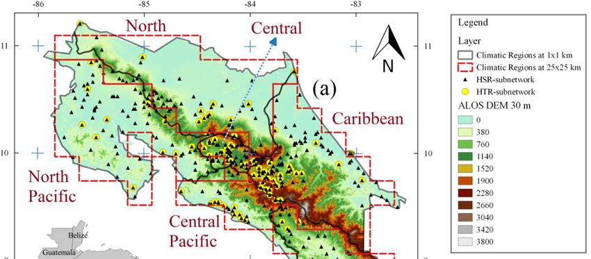
Water 2019, 11, 70                                                                                      2 of 22

1. Introduction
      Precipitation climatologies represent the foundation of climate research in a variety of sectors,
including agriculture, forestry, water resources management, hydrological and hydrogeological
modelling, urban planning, flood inundation and biodiversity management; all of which need to adapt
to future Climate Change impacts [1–3]. Precipitation climatologies have extensively been used to
evaluate general circulation models (GCMs) and regional climate models (RCMs) by comparing their
outputs to observational data sets [4,5]. The generation of precipitation climatologies is generally based
on data coming from rain-gauge observational networks, which are recurrently sparse and unevenly
distributed in many regions of the World [6]. Furthermore, historical records observed through these
networks are frequently incomplete because of missing data during the observed period or insufficient
number of stations in the study region [7,8].
      The absence of homogeneous and continuous historical records can considerably limit the
scope of local climate impact studies over specific areas of interest [9]. The reasons for such
discontinuities include relocation of the observation stations, equipment and data-acquisition failure,
cost of maintenance and changes in the surrounding environment due to anthropogenic or natural
causes [10–12], which has motivated climatologists to re-examine historical weather-station records.
      Rain-gauge observational networks are constructed with the intention of providing measurements
that adequately characterize most of the non-trivial spatial variations of precipitation [13,14]. This
is hard to accomplish if only continuous and regular observational networks are included in the
generation of such climatologies. The situation becomes more severe in tropical regions, due to high
spatial and temporal variability and scarce data availability [15].
      On that premise, some climatologists may choose to favour a high spatial resolution (HSR)
network by maximizing the amount of temporally discontinuous, irregularly distributed rain-gauges
at the expense of reducing the extent to which the station records are lengthy and temporally
commensurate [16]. On the contrary, a different group of climatologists may favour a high temporal
fidelity by promoting a high temporal resolution network (HTR) at the expense of reducing the number
of rain-gauges and, therefore, their ability to spatially resolve the climatic field of interest [17,18]. This
is done by selecting records that are sufficiently long and temporally commensurate within a regularly
distributed, temporally continuous network.
      To this end, various attempts have been made to develop and improve global and regional gridded
precipitation datasets, but they usually suffer from the lack of sufficient rain-gauge observational
densities [19–21]. Nonetheless, historical records coming from rain-gauge observational networks
even when discontinuous and irregular, represent the most reliable source of climatic information
prior to the emergence of remote sensing products, and therefore continue to comprise the bases of
most credible estimates for generating long-term time series of areal precipitation [6,22].
      The reconstruction of precipitation climatologies largely relies on the application of spatial
interpolation methods on data recorded by such observational networks [23]. Spatial interpolation
is achieved by estimating a regionalized value at unsampled points from weights of observed
regionalized variables. Interpolation methods can broadly be classified as either deterministic or
geostatistical [24]. The fundamental principle behind deterministic methods is that the relative weight
of an observed value decreases as the distance from the prediction location increases. Geostatistical
methods however, are based on the theory of regionalized variables, and provide a set of statistical
tools for incorporating the spatial correlation of observations in the data processing. Some authors
have criticized deterministic methods since they are unable of accounting for temporal and spatial
disaggregation [4]. Geostatistical methods, in contrast, have the capability of incorporating covariants
fields, which are in principle denser than point field observations [25]. The relevant secondary
information supplied by covariants can potentially improve interpolation results as long as they
exhibit a strong correlation with the interpolated field [26]. Among such covariants, elevation has
commonly been used [27,28].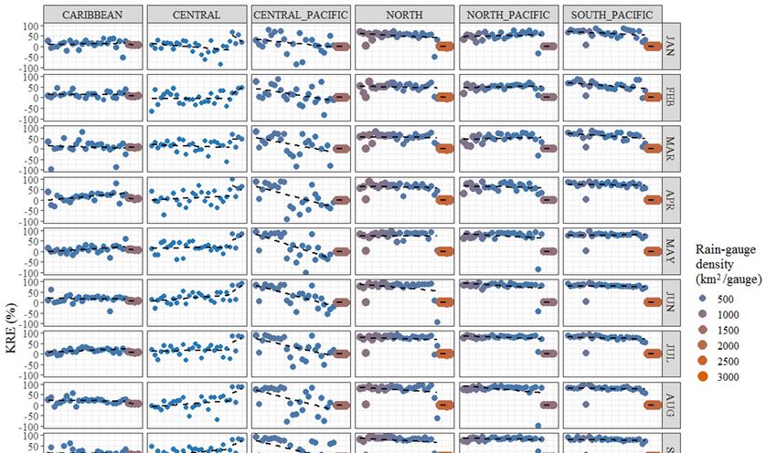
Water 2019, 11, 70                                                                                 3 of 22

      Different interpolation methods lead to different errors depending on the realism of the
assumptions on which they rely [29]. Geostatistical methods rely on the assumption of data stationarity,
which requires normal distribution and homogeneous variance of the field variable [30]. Precipitation
is a highly skewed, heteroscedastic and intermittent field in nature and therefore frequently contradicts
the assumptions of data normality. This forces data transformation using analytical or numerical
techniques, which cannot always satisfy the assumptions on normality and homoscedasticity [31].
Geostatistical interpolation methods nonetheless, have broadly been applied in the design, evaluation
and monitoring of rain-gauge observational networks. Among such methods, kriging is one of
the most popular geostatistical interpolation techniques—widely accepted due to its relatively low
computational cost and its flexibility regarding input and output data [14]. When using kriging,
several outputs can be generated besides the prediction field; this includes the estimation of the
residual errors and the kriging variance. Kriging variance is also estimated on points where no
observations exist and, consequently, provides a spatial view on the measure of performance [32].
Various methods of rain-gauge network performance have been developed using kriging interpolation
techniques. For such methods, known as variance-reduction techniques, the performance evaluation
of a rain-gauge network focuses on reducing the error variance of the average field value over a certain
domain [33–35]. Most of these techniques take into account the number and location of rain-gauges
to yield greater accuracy of areal precipitation estimation with minimum cost. Bastin et al. [33]
used the kriging variance as a tool in rain-gauge network-design for optimal estimation of the
areal average precipitation. The authors developed an iterative screening procedure that selected
rain-gauges associated with the minimum kriging variance. Consequently, all available rain-gauges
are prioritized and this information is used for adding or deleting rain-gauges within the network.
Similarly, Kassim and Kottegoda [34] prioritized rain-gauges with respect to their contribution in
kriging variance reduction in a rain-gauge network through comparative kriging methods. By contrast,
Chebi et al. [35] developed a robust optimization algorithm blending kriging variance reduction
and simulated-annealing to expand an existing rain-gauge network by considering Inverse Distance
Weighting (IDF) curve-parameters evolution, which ultimately allowed the authors to optimally locate
new rain-gauges in imaginary locations.
      Consequently, the concept of kriging variance-reduction could also be used to determine whether
a HSR rain-gauge network could yield a more accurate estimate of a point precipitation average than a
HTR rain-gauge network for the same time step and region. If by using a HSR rain-gauge network,
which is most likely temporally discontinuous and irregularly distributed over a certain domain for
a specific time step, the resulting average interpolated precipitation yields a lower kriging variance,
it is probably wiser to increase the density of the rain-gauge network at the expense of temporal
fidelity by including more stations, even though their records may not exactly represent the same time
step. This is of the utmost importance for the reconstruction of precipitation climatologies in many
regions of the world, where rain-gauge network-densities, as well as their temporal resolution, are
far from optimal [13]. As stated in the regional projection of the Fourth Assessment Report of the
Intergovernmental Panel on Climate Change [36], Central America is one of the regions in the world
that most likely will experience an important decrease in mean annual precipitation in the following
decades. This trend has already been identified by previous Climate Change regional studies focusing
on the Central American corridor [36–38]. In consequence, there is a heightened need to generate
quality precipitation climatologies for such regions, even on the grounds of data-sparse discontinuous
and irregular rain-gauge observational networks.
      This research focuses on Costa Rica, Central America, where most of the territory has experienced
some degree of precipitation change during the period 1961–1990, showing increases on the
north-western Caribbean side and decreases on the Pacific side [39,40]. Accordingly, the objective
of this study is to determine whether a high spatial resolution (HSR) rain-gauge network yields a
more accurate estimate of average precipitation than a high temporal resolution (HTR) rain-gauge
network, based on the application of kriging variance-reduction techniques. The performance of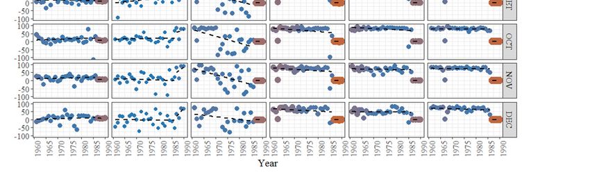
Water 2019, 11, 70 4 of 22
various interpolation methods in the generation of monthly precipitation climatologies for the period
1961–1990 is then evaluated for all climatic regions of Costa Rica. Finally, the generated climatologies
are validated against publicly available global precipitation datasets, including those from the Global
Water 2019, 11, x Climatology
Precipitation FOR PEER REVIEW
Centre (GPCC), the Climate Research Unit (CRU) and WorldClim. 4 of 23
2. Materials and Methods
2.1. Study
2.1. Study Area
Area
Costa Rica is located across the Central American isthmus between Panama and Nicaragua at
almost its
its narrowest
narrowestpoint
point(Figure
(Figure1b).
1b).The
Thecountry
countryis is
bordered byby
bordered thethe
Caribbean SeaSea
Caribbean to the easteast
to the andand
the
Pacific Ocean to the west, which favours oceanic and climatological influences from both oceans.
the Pacific Ocean to the west, which favours oceanic and climatological influences from both oceans. Costa
Rica occupies an areaanof area
51,060 2 and is 2meridionally divided by northwest-southeast trending
Costa Rica occupies ofkm
51,060 km and is meridionally divided by northwest-southeast
cordilleras of different topographic complexity which risewhich
trending cordilleras of different topographic complexity to over 3400
rise m (Figure
to over 1a).
3400 m (Figure 1a).
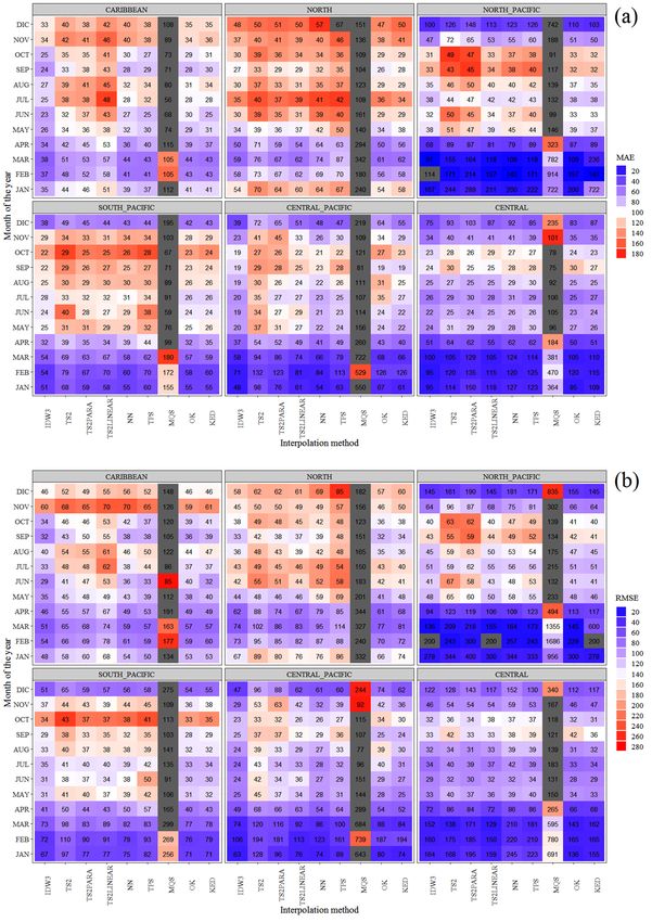
Figure 1. (a) Location of rain-gauge and Digital Elevation Model (DEM) for each climatic region in
Costa Rica during the period 1961–1990. (b) Position of Costa Rica in Central America.
Coastlines and
Coastlines andcordilleras
cordillerashowever,
however, do not
do run
not parallel to one to
run parallel another, thus displaying
one another, increased
thus displaying
widths and elevations towards the south-east territory [41]. Precipitation variability
increased widths and elevations towards the south-east territory [41]. Precipitation variability in Costa Rica in
is
driven by interactions between the local topography and a combination of the seasonal
Costa Rica is driven by interactions between the local topography and a combination of the seasonal migration of
the intertropical
migration of the convergence zoneconvergence
intertropical (ITCZ), which includes
zone (ITCZ),sea breeze
which effects,
includes monsoonal
sea breezecirculations,
effects,
strong easterly trade winds, cold air masses from mid-latitudes in the
monsoonal circulations, strong easterly trade winds, cold air masses from mid-latitudes winter and the perturbing
in the
influences
winter andofthehurricanes
perturbingand tropical of
influences cyclones in the
hurricanes andAtlantic
tropicalOcean [42].in The
cyclones complexOcean
the Atlantic pattern of
[42].
precipitation regimes apparent in the country reflects influences at a variety of
The complex pattern of precipitation regimes apparent in the country reflects influences at a varietygeographic scales.
The temporal scales.
of geographic and spatial variability
The temporal andofspatial
precipitation
variabilityin the country is heavily
of precipitation influenced
in the country by El
is heavily
Niño-Southern
influenced by ElOscillation (ENSO),
Niño-Southern which complex
Oscillation (ENSO),responses
which complex(warmresponses
or wet) vary in terms
(warm or wet)of their
vary
signs, magnitudes, duration and seasonality between those areas draining towards
in terms of their signs, magnitudes, duration and seasonality between those areas draining towards the Pacific and
those draining towards the Caribbean. Consequently, mean monthly precipitation
the Pacific and those draining towards the Caribbean. Consequently, mean monthly precipitation exhibits a strong
seasonalacycle
exhibits strongand regional
seasonal variability
cycle [43], variability
and regional which can[43], be observed
which canbybethe monthly
observed byprecipitation
the monthly
precipitation derived from all available rain-gauge stations for the period 1961–1990 (Figure 2).
Accordingly, the Instituto Meteorológico de Costa Rica (IMN) [44] has divided the Costa Rican
territory into six separate climatic regions: North, Caribbean, North-Pacific, Central-Valley,
Central-Pacific and South-Pacific, in which northeastern and southwestern domains are determined
by the position and elevation of the aforementioned cordilleras (Figure 1a). These established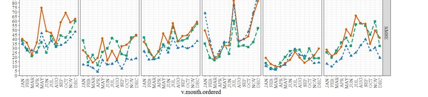
Water 2019, 11, 70                                                                                                   5 of 22

derived from all available rain-gauge stations for the period 1961–1990 (Figure 2). Accordingly, the
Instituto Meteorológico de Costa Rica (IMN) [44] has divided the Costa Rican territory into six separate
climatic regions: North, Caribbean, North-Pacific, Central-Valley, Central-Pacific and South-Pacific, in
which northeastern and southwestern domains are determined by the position and elevation of the
aforementioned      cordilleras
Water 2019, 11, x FOR           (Figure 1a). These established regions reflect the separation that elevation
                      PEER REVIEW                                                                       5 of 23
imposes between Caribbean (northeastern) and Pacific (southwestern) sources of moisture and also
reveals  the local
controlling    important   role played
                     precipitation  [45]. by elevation
                                          This enables in controlling
                                                       important      localinto
                                                                  insights  precipitation [45]. characterized
                                                                                local climates,  This enables
important
by diverse insights    into local climates,
              and heterogeneous              characterized by diverse and heterogeneous land surfaces.
                                    land surfaces.

      Figure 2. Mean monthly precipitation derived from all available rain-gauge stations for each climatic
      region in Costa Rica during
                           during the
                                  the period
                                      period 1961–1990.
                                             1961–1990. Error
                                                        Error bars
                                                              bars represent
                                                                   represent the
                                                                              the standard
                                                                                  standard deviation.
                                                                                           deviation.

2.2. Datasets and
2.2. Datasets and Data
                  Data Transformation
                       Transformation
      Aggregated      monthlyprecipitation
      Aggregated monthly         precipitationdata datawere
                                                        were    provided
                                                             provided     by by    Instituto
                                                                               Instituto       Meteorológico
                                                                                          Meteorológico          of Costa
                                                                                                            of Costa    Rica
Rica
(IMN) for the period 1961–1990. A total of 416 rain-gauge stations were active during this during
      (IMN)     for  the  period    1961–1990.      A  total   of 416    rain-gauge      stations   were  active    period
this period throughout
throughout     the country,the  butcountry,   but their
                                     their spatial        spatial distribution
                                                     distribution     is irregularisand irregular
                                                                                            not alland   not all
                                                                                                     stations     stations
                                                                                                                registered
registered  continuously     or records   were  not  temporally    commensurate.
continuously or records were not temporally commensurate. Consequently, two rain-gauge  Consequently,    two   rain-gauge
sub-networks
sub-networks were weredefined
                         defined (Figure  1a):1a):
                                    (Figure    a high  temporal
                                                    a high         resolution
                                                              temporal            sub-network
                                                                            resolution            (HTR), which
                                                                                          sub-network     (HTR),includes
                                                                                                                     which
stations
includespossessing     at least 20 at
           stations possessing      years
                                      leastof20
                                              continuous    records during
                                                years of continuous              the study
                                                                           records    duringperiod   (157 in
                                                                                               the study     total);(157
                                                                                                           period     andina
high  spatial  resolution   sub-network     (HSR),   which    includes    all HTR-stations      plus
total); and a high spatial resolution sub-network (HSR), which includes all HTR-stations plus those  those  stations   with
less thanwith
stations   20 years
                 less of continuous
                      than   20 years records     (416 in records
                                        of continuous      total). Stations
                                                                     (416 in included      in the included
                                                                                total). Stations   HTR networkin thehadHTRat
least 90%had
network     of available   monthly
                at least 90%          records
                               of available     during records
                                              monthly    the 20-year    defined
                                                                   during           temporal
                                                                             the 20-year        window.
                                                                                            defined       Therefore,
                                                                                                     temporal    window. the
number    of stations  used   at each  time   step  varies  over  time   within    both  sub-networks,
Therefore, the number of stations used at each time step varies over time within both sub-networks,        with  the   HTR
providing
with the HTRthe most    commensurate
                  providing               long-term monthly
                              the most commensurate                records.
                                                            long-term     monthly records.
      An  analysis  of the  temporal   evolution    of both  sub-networks
      An analysis of the temporal evolution of both sub-networks                across  all climatic
                                                                                    across            regions
                                                                                            all climatic       shows
                                                                                                          regions       that
                                                                                                                     shows
precipitation    data  were  collected   from   a constantly    changing      configuration     during
that precipitation data were collected from a constantly changing configuration during the entire       the  entire   study
study period, which peaks in the mid-1970s and starts to decrease in the mid-1980s, with a drastic
drop after 1987, when many stations all around the country were either abandoned or relocated
(Figure 3). The HSR sub-network satisfies World Meteorological Organization (WMO) standards of
250 km2/gauge for mountainous areas [46] in the Caribbean, Central-Valley and Central-Pacific
regions during most of the 1970s and 1980s, with the Central-Pacific not reaching the minimum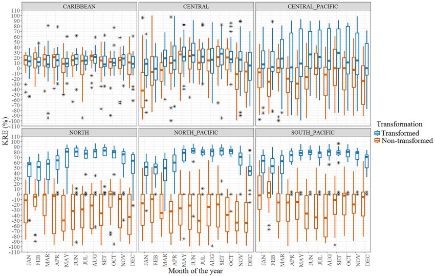
Water 2019, 11, 70 6 of 22
period, which peaks in the mid-1970s and starts to decrease in the mid-1980s, with a drastic drop after
1987, when many stations all around the country were either abandoned or relocated (Figure 3). The
HSR sub-network satisfies World Meteorological Organization (WMO) standards of 250 km2 /gauge
for mountainous areas [46] in the Caribbean, Central-Valley and Central-Pacific regions during most of
the 1970s and 1980s, with the Central-Pacific not reaching the minimum value during most of the 1960s.
North, North-Pacific
Water 2019, 11, x FOR PEERand South-Pacific regions, however, barely reach that standard during most
REVIEW 6 ofof
23
the 1970s and 1980s, with the North region being the most critically instrumented area, particularly
during most ofWMO
only satisfies the 1960s. In contrast,
standards for thethe HTR sub-network
Central-Valley region,only satisfies
since WMOstations
rain-gauge standards for the
seemed to
Central-Valley
concentrate in region,
the since
most rain-gauge
populatedstations
regionseemed
of theto country.
concentrate in the1987,
After most however,
populated region
only the of
the country. After
Central-Valley 1987,satisfies
region however, onlystandards.
WMO the Central-Valley
All otherregion satisfies
regions are wayWMO standards.
above the 250 kmAll2/gauge
other
regions areregardless
way aboveofthe 250orkm 2 /gauge after 1987 four
regardless of HSR or HTR, as there barely four
after 1987 HSR HTR, as there barely operational stations in each region. Quality
operational
control of thestations
IMN in each region.data
precipitation Quality control of the
was undertaken toIMN precipitation
identify data was undertaken
possible systematic or acquisition to
identify possible systematic
errors and extreme outliers. or acquisition errors and extreme outliers.
Figure3.3. Temporal
Figure Temporalevolution
evolutionofofInstituto
InstitutoMeteorológico
Meteorológicode deCosta
CostaRica
Rica(IMN)
(IMN)rain-gauge
rain-gaugenetwork
network
density 2
density(km
(km2/gauge)
/gauge) for each climatic region
region during
during the
the period
period1961–1990.
1961–1990. Black
Blackdashed-lines
dashed-linesmark
mark
WMO 22
WMOdensity
densitystandards
standardsfor
formountainous
mountainousareas
areas(250
(250km
km/gauge).
/gauge).
Since
Sincegeostatistical
geostatisticalinterpolation
interpolationmethods relyrely
methods on the assumption
on the of data
assumption normality,
of data records
normality, from
records
both rain-gauge sub-networks were transformed using the Box–Cox optimization technique
from both rain-gauge sub-networks were transformed using the Box–Cox optimization technique [47] to
correct for non-Gaussianity
[47] to correct and approximate
for non-Gaussianity normality.
and approximate The transformation
normality. is dependent
The transformation on the
is dependent on
parameter Lambda only (λ).
the parameter Lambda only (λ). (
Y λ −1
λ 6= 0
log Y∗ =
Y (Y) 1 λ = 0
λ (1)
0
Y* (1)
where Y and Y* are the original and transformed variables, respectively; λ is the
log(Y ) 0
transformation parameter.
Box–Cox
where Y and transformation was and
Y* are the original individually applied
transformed to HSRrespectively;
variables, and HTR datasets fortransformation
λ is the each climatic
region at
parameter.a monthly basis, prior to the application of kriging interpolation. As suggested by
ErdinBox–Cox
et al. [48]transformation
and Woldemeskelwasetindividually
al. [49], possible values
applied for “λ”
to HSR andwere
HTRconstrained
datasets fortoeach
a minimum
climatic
region at a monthly basis, prior to the application of kriging interpolation. As suggested by Erdin et
al. [48] and Woldemeskel et al. [49], possible values for “λ” were constrained to a minimum value of
0.2 in order to avoid excessive data transformation. Precipitation estimates and kriging variance
were subsequently back-transformed to their original units (mm/months). Logarithmic
transformation was not considered because of the impossibility of transforming zero values. Kriging
Water 2019, 11, 70 7 of 22
value of 0.2 in order to avoid excessive data transformation. Precipitation estimates and kriging
variance were subsequently back-transformed to their original units (mm/months). Logarithmic
transformation was not considered because of the impossibility of transforming zero values. Kriging
variance was also calculated using the raw non-transformed data for comparison purposes.
2.3. Kriging Variance Reduction Efficiency
Ordinary kriging (OK) is one of the most popular kriging estimators and can be described as a
weighted average interpolation [30], where estimated values at target locations are calculated taking
into account the distance of the neighbouring observed values to the location of the point to be
estimated according to:
n
Ẑ ( X0 ) = ∑ λ i Z ( Xi ) (2)
i =1
where Ẑ is the estimated value at an unobserved location X0 , Z is the observed value at the sampled
location, Xi and λi are the kriging weights.
OK weights for sampled values are calculated based on the parameters of a variogram model,
which provides the best linear unbiased estimator of point values with minimum error variance [15]
according to:
2
1 n
γ̂(h) = ∑
2n i=1
[ Z ( Xi ) − Z ( Xi + h)] (3)
where γ̂ is the semivariance as a function of distance, h is the distance separating sampled points and
n is the number of pairs of sampled points.
A plot of γ̂(h) against h is known as the observational variogram. Standard variograms models
can then be fitted to the observations. OK weights are determined such as to minimize the estimation
of the kriging variance: h
2 i
Var Ẑ ( X0 ) = E Ẑ ( X0 ) − Z ( X0 ) (4)
where Var is the kriging variance and Z(X0 ) is the true value expected at point X0 .
OK weights are finally calculated by relating the semivariance γ̂ to a system of linear equations
known as the ordinary kriging system (OKS):
n
∑ λi γ̂(di j ) + µ = γ̂(di0 ); f orj = 1, . . . n
i =1 (5)
n
∑ λi = 1
i =1
where γ̂ di j and γ̂(di0 ) indicate the variogram values that come from the standard variogram models
for the distance dij and di0 respectively, dij is the separation distance between sampling points Xi and
Xj , di0 is the separation distance between the sampling point Xi and the target location, and µ is the
Lagrange multiplier.
The robustness of OK significantly depends on the proper selection of standard variograms
models that quantify the degree of spatial autocorrelation in the dataset [24]. Since the duration,
magnitude and intensity of precipitation events vary across space and time, it is not realistic to
adopt a unique variogram for all precipitation events, irrespective of seasonal and meteorological
conditions [14]. Thus, selecting an appropriate model to capture the features of the data is critical [9].
Variogram fitting should reflect specific spatial structures of particular time lapses and therefore, the
use of stationary variograms should be avoided. In this study, parameters values of the range, nugget
and sill for standard variograms models (Spherical (Sph), Exponential (Exp), Gaussian (Gau), Matern
(Mat) and Matern–Stein (Sten)) were automatically and individually fitted to HTR and HSR datasets at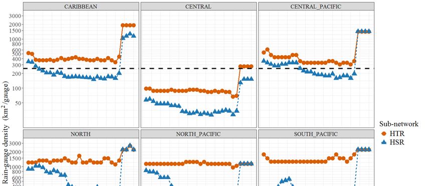
Water 2019, 11, 70                                                                                   8 of 22

each time step, such as to minimize the weighted sum of squares of differences between experimental
and model variogram values:
                                             n                            2
                                    WSS =   ∑ ω (hi )[γ̂(hi ) − γ(hi )]                                 (6)
                                            i =1

where γ is the experimental semivariance, γ̂ is the model semivariance, h is the distance separating
sampled points and ω is the relative weight assigned as a function of distance.
      To assess whether the HSR sub-network yielded a lower kriging variance than the HTR
sub-network for the same time step, the kriging variance reduction efficiency (KRE) function of
the spatially-averaged kriging variance between the two sub-networks was employed for each of the
six climatic regions, according to:
                                                                        !
                                     Var HTR Ẑ ( X0 ) − Var HSR Ẑ ( X0 )
                           KRE =                                            100                       (7)
                                              Var HTR Ẑ ( X0 )

where KRE is the kriging variance reduction efficiency (%), Var HTR is the HTR spatially averaged
kriging variance and Var HSR is the HSR spatially averaged kriging variance.
     Positive KRE values for a certain climatic region and time step indicate that the HSR sub-network
yields a more accurate estimate of a point precipitation average than the HTR sub-network. Negative
values indicate the opposite. KRE was also calculated using the raw non-transformed data for
comparison purposes.

2.4. Interpolation Methods and Experimental Setup
      Deterministic and geostatistical interpolation methods (Table 1) were selected to produce spatially
continuous precipitation climatologies for each climatic region of Costa Rica during the period
1961–1990 based on datasets from the HSR sub-network only (Figure 1a). All spatial interpolation and
data processing was executed using the R programming language (v3.5.2) [50] along with specialized
R packages. Geostatistical modelling, spatio-temporal data analysis and raster generation were
implemented by combining functionalities of the gstat (v1.1.6), sp (v1.3.1), raster (v2.8.4), RSAGA
(v1.3.0) and rgdal (v1.3.6) packages. Since the spatial structure of precipitation data varies in space and
time, OK automatic variogram fitting analysis was conducted separately for each sub-network and
climatic region at a monthly time step using the R packages automap (v1.0.14), which minimizes the
weighted sum of squares of differences between experimental and model semivariogram (Equation
(1)). All distances were calculated according to the official Costa-Rica Transverse-Mercator (CRTM05)
projected-coordinate-system using a spatial grid resolution of 1 × 1 km, which was selected primarily
on the grounds of computational costs. The selected interpolation methods were chosen on the basis of
(a) previous use in meteorology and climatology applications [13,24,51–53]; (b) continuity of recorded
data; (c) location and distribution of available rain-gauges and (d) computational cost. Topographic
information was derived from the Advanced Land Observing Satellite (ALOS) AW3D-30 m (30) Digital
Elevation Model (DEM), which was subsequently resampled to a 1 × 1 km spatial resolution using the
bilinear resampling technique. The R-code, raw-data, results and ggplot2 graphic-code are presented
in Supplementary Materials. As recommended by Daly et al. [26], resampled elevation from the
DEM was preferred over the actual station elevations points to improve spatial representation and
generalization of orographic and convective precipitation mechanisms.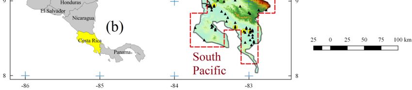
Water 2019, 11, 70                                                                                           9 of 22

                        Table 1. Selected interpolation methods and relevant R packages.

         Abbreviation                   Method                            R_package             Class
             IDW              Inverse Distance Weighting            gstat, sp, raster       Deterministic
              TS2          Trend surface, 2nd. polyn. surface       gstat, sp, raster       Deterministic
           TS2PARA         Trend surface, 2nd. parab. surface       gstat, sp, raster       Deterministic
          TS2LINEAR        Trend surface 2nd planar surface         gstat, sp, raster       Deterministic
              TPS                  Thin Plate Spline             gstat, sp, raster, rsaga   Deterministic
             MQS              Modified Quadratic Shepard         gstat, sp, raster, rsaga   Deterministic
              NN                  Nearest Neighbour              gstat, sp, raster, rsaga   Deterministic
              OK                   Ordinary Kriging              gstat, raster, automap     Geostatistical
             KED              Kriging with External Drift        gstat, raster, automap     Geostatistical

2.5. Performance Assessment of the Interpolation Methods
     Performance of the various spatial interpolation methods was evaluated using a leave-one-out
cross validation (LOOCV) technique on the HSR network only (Figure 1a). Cross validation statistics
serve as diagnostic tools to determine whether the performance of the selected interpolation method
was acceptable. In LOOCV, a subset of stations from the entire data set is temporarily removed and the
values at the same locations are estimated using the remaining stations (in this case, 25% of the stations
without repetitions). LOOCV was sampled randomly with no data repetition due to the temporal
discontinuities of the HSR sub-network. The procedure was repeated until all the stations in the data
set were temporarily removed in turn and estimated. Cross validation was limited to the period
1961–1987 for all climatic regions except for the Central-Valley and Caribbean regions, since after
1987 there were not sufficient stations to properly calculate semi-variograms for OK and KED. Two
indicators were used to quantitatively compare interpolated estimates against rain-gauge observations,
the mean absolute error (MAE) and the root-mean square error (RMSE) according to:

                                                      1 n
                                                      n i∑
                                            MAE =           | Pi − Oi |                                         (8)
                                                         =1
                                                v
                                                u1 n
                                                u               2
                                         RMSE = t ∑ ( Pi − Oi )                                                 (9)
                                                  n i =1

where Pi and Oi are the predicted and observed values respectively.
     The MAE is an absolute measure of bias that varies between 0 to +∞. A MAE value close to 0
indicates an unbiased prediction. The RMSE ranges from 0 to +∞, and it is used for checking the
estimation accuracy between observed and predicted values. A RMSE value close to 0 indicates a
higher accuracy in estimation. The two indicators were calculated at each time step and presented as
monthly average for each climatic region.

2.6. Validation Datasets
     The Global Precipitation Climatology Centre (GPCC), the Climate Research Unit (CRU), and
WorldClim global precipitation datasets were used to assess the performance of the generated IDW
climatology for all climatic regions of Costa Rica based on data from the HSR network (Figure 1a). The
full GPCC version 2018 dataset [21], which covers the period 1891–2016 at a 0.25◦ spatial resolution
(~25 km), is the most accurate in situ centennial monthly global land-surface precipitation product
of GPCC. It is based on the ~80,000 stations worldwide that feature record durations of 10 years or
longer. The data coverage per month varies from ~6000 (before 1900) to more than 50,000 stations.
Since GPCC covers the period 1891–2016, monthly totals were isolated for the period 1961–1990 only.
The CRU-CL version 2.0 monthly precipitation dataset [19], which covers the period 1961–1990 with a
spatial resolution of 10 min (~18.5 km), was constructed based on observations of a number of sources
including national meteorological agencies and archive centres, the WMO and the International Centre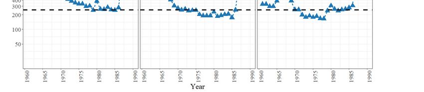
Water 2019, 11, 70                                                                                   10 of 22

for Tropical Agriculture (CIAT). The CRU-CL includes not only precipitation but also temperature
and relative humidity among other variables. The WorldClim version 1.0 monthly precipitation
dataset [20], which was generated through interpolation of average monthly climate data from weather
stations, covers the period 1960–1990 and was distributed at spatial resolutions of 30 arc-s, 10 min,
5 min and 2.5 min. Major climate databases used in the generation of WorldClim include the Global
Historical Climatology Network (GHCN), the Food and Agriculture Organization of the United
Nations (FAO), the WMO, the International Centre for Tropical Agriculture (CIAT) and a number of
additional national databases. For comparison purposes, all global precipitation datasets, along with
the final IDW-generated climatology for Costa Rica, were resampled to a 25 × 25 km spatial resolution
using the bilinear resampling technique; mainly selected on the basis of the GPCC 0.25◦ (~25 km)
original spatial resolution (Figure 1a). The resulting spatially averaged time series were analysed for
each climatic region using the mean absolute error (MAE), the root-mean square error (RMSE) and the
Pearson’s correlation coefficient (CORR), intended to quantify the goodness of fit between the local
precipitation climatology and the aforementioned global datasets.

3. Results and Discussion

3.1. Kriging Reduction Efficiency
     Monthly box-plots of the kriging reduction efficiency (KRE) for the period 1961–1990 show
significantly diverse responses among all climatic regions for both transformed and non-transformed
datasets (Figure 4). Concerning transformed datasets, KRE returns predominantly positive values
throughout most of the study period regardless of the climatic region, which proves that in most cases,
the HSR sub-network yields lower kriging variance than the HTR sub-network for the same time
step. As kriging variance greatly depends on parameters derived from standard-variograms (range,
nugget and sill), which fitting reflects specific spatial structures of particular time steps; predominantly
KRE positive values suggest that variograms derived from the HTR sub-network are insufficient
to properly represent the regional variability of monthly precipitation. In consequence, the HSR
sub-network captures a more detailed spatio-temporal distribution of the precipitation patterns over
most climatic regions of Costa Rica, even when the network is temporally discontinuous and irregularly
distributed. Despite the HTR sub-network providing the most commensurate, long-term monthly
precipitation records, its density remains below WMO standards for mountainous areas (Figure 3),
which is particularly vulnerable in the analysis and modelling of spatio-temporal climatic variability.
     Specifically, the North, North-Pacific and South-Pacific regions show entirely positive values and
similar KRE quantile distributions throughout the study period, with lower median values during the
driest months (JFMA) and a tendency to increase as average precipitation also increases. KRE then
stabilizes during the wettest months (June through October) with narrower quantile distributions, to
finally decrease again at the end of November. This implies that KRE is more effective during the
wet season than during the dry season for these regions, with the North-Pacific and South-Pacific
regions draining towards the Pacific Ocean and the North region discharging towards the Caribbean
Sea (Figure 1a). The Central-Pacific region nonetheless, even when draining directly towards the
Pacific Ocean, exhibits a considerable distinct KRE behaviour when compared to the North-Pacific
and South-Pacific regions, since quantile distributions spread over the entire range (−100% to 100%)
indistinctly of dry or wet months (Figure 4).
precipitation. In consequence, the HSR sub-network captures a more detailed spatio-temporal
distribution of the precipitation patterns over most climatic regions of Costa Rica, even when the
network is temporally discontinuous and irregularly distributed. Despite the HTR sub-network
providing the most commensurate, long-term monthly precipitation records, its density remains
below
Water WMO
2019, 11, 70 standards for mountainous areas (Figure 3), which is particularly vulnerable 11
inofthe
22
analysis and modelling of spatio-temporal climatic variability.
4. Kriging
Figure 4. Kriging reduction efficiency
efficiency (KRE)
(KRE) for
for transformed
transformed and
and non-transformed
non-transformed datasets
datasets for
for each
each
climatic region
region during
during the
the period
period 1961–1990.
1961–1990. Points
Points marked
marked with
with (*)
(*) symbol
symbol represent
representoutliers.
outliers.
During the months
Specifically, of April,
the North, May andand
North-Pacific December, whichregions
South-Pacific represent the entirely
show transition between
positive the
values
dry and wet seasons, nearly 50% of the observations reach negative values as
and similar KRE quantile distributions throughout the study period, with lower median values does October (the
wettest month)
during the formonths
driest the Central-Pacific
(JFMA) and region. Thisto
a tendency region exhibits
increase higherprecipitation
as average network densities than the
also increases.
North-Pacific or South-Pacific regions, but the HTR sub-network is highly concentrated
KRE then stabilizes during the wettest months (June through October) with narrower quantile along the
Pacific coastline, with only a few stations in the mountainous areas (Figure 1a).
distributions, to finally decrease again at the end of November. This implies that KRE is moreThis configuration
suggests that during
effective during theseason
the wet analysed
thanperiod
during(1961–1990),
the dry seasonthefor
Central-Pacific
these regions,sub-network captured
with the North-Pacific
spatially localized precipitation events throughout the year, which complex responses
and South-Pacific regions draining towards the Pacific Ocean and the North region discharging vary in terms
of their magnitudes, duration and seasonality. The occurrence of spatially localized precipitation
events is exacerbated by various climatic effects associated to the intertropical convergence zone
(ITCZ) [41,42], which most certainly occur at daily or hourly time scales and are ultimately aggregated
into monthly timescales. Subsequently, HTR fitted variograms exhibit lower nugget, lower sill and
shorter ranges values as compared to their HSR counterpart, which nevertheless is applicable to
the entire Central-Pacific region. To illustrate such situation, the HTR and HSR fitted variograms
for August 1971 are compared (Figure 5). In this case, the kriging-standard-error (square root of
the kriging variance) for the HTR sub-network (expressed in mm/month) tends to represent only
a small and localized fraction of the Central-Pacific coastline (Figure 5a), whereas the same metrics
are more spatially distributed for the HSR sub-network (Figure 5b). In consequence, even when the
average kriging variance for the HTR sub-network (0.112) is lower than its HSR counterpart (0.136),
which results in a negative KRE value (−21.401%), the metrics seem to be spatially biased due to the
abovementioned concentration of rain-gauge stations near the Pacific coastline. The presence of KRE
negative values in the Central-Pacific region should not suggest that the HTR sub-networks yield
a more accurate estimate of a point precipitation average than the HSR sub-networks do, since this
tendency is highly variable and does not replicate during the entire period of analysis. In summary,
OK is unable to explain a high portion of the spatial variability within the Central-Pacific region if
only stations from the HTR sub-network are included. Similar arguments can be used to explain the
presence of scattered KRE negative values in the Caribbean and Central-Valley regions, both of which
have the highest and more temporally stable network densities of all climatic regions (Figure 3).sub-networks do, since this tendency is highly variable and does not replicate during the entire
period of analysis. In summary, OK is unable to explain a high portion of the spatial variability
within the Central-Pacific region if only stations from the HTR sub-network are included. Similar
arguments can be used to explain the presence of scattered KRE negative values in the Caribbean
and2019,
Water Central-Valley
11, 70 regions, both of which have the highest and more temporally stable network
12 of 22
densities of all climatic regions (Figure 3).
Figure5.5.Kriging
Figure Krigingprediction,
prediction,kriging-standard-error
kriging-standard-error and
and fitted
fitted variogram
variogram for the HTR (a) and HSR (b)
sub-networks for August
(b) sub-networks 1971.
for August Central-Pacific
1971. climatic
Central-Pacific region,
climatic Costa
region, Rica.
Costa Rica.
In the case of the Central-Valley region, in agreement to the Central-Pacific region; the transitional
months of April and December show the widest KRE quantile distributions, with a clear tendency
to stabilize during the wettest months (May to November). Similar to the North, North-Pacific and
South-Pacific regions, KRE is more effective during the wet season than during the dry season for the
Central-Valley region. In this case, the incidence of higher network densities does not prevent the
presence of KRE negative values during the driest months.
On the other hand, performance of the kriging variance-reduction (KRE) noticeably benefited
from the Box–Cox optimization technique when applied to the North, North-Pacific, South-Pacific
and Central-Pacific regions, since in most cases non-transformed datasets produced predominantly
negative KRE values regardless of dry or wet months (Figure 4), which proves that data transformation
did improve Gaussianity of the precipitation field. Furthermore, for the North, North-Pacific and
South-Pacific regions, interquartile ranges are hardly distinguishable for most non-transformed
boxplots, indicating that precipitation is a highly skewed, heteroscedastic and intermittent field
in nature, which usually contradicts the assumptions of data normality [31]. This seems particularly
evident in Costa Rica, as mean monthly precipitation exhibits a strong seasonal cycle and regional
variability (Figure 2). Data transformation, nonetheless, is not as beneficial for the Caribbean and
Central-Valley regions, both of which exhibit the highest network densities (Figure 3). On one hand,
non-transformed KRE values outperform their corresponding transformed counterpart during the
wettest months (May to October) for the Central-Valley region. The opposite situation occurs during the
driest months. On the other hand, the Caribbean region, which exhibits the most persistent year-round
precipitation regime (Figure 2), shows little gain in applying data transformation, suggesting a more
normally distributed spatial pattern as compared to the remaining climatic regions. In summary, data
transformation seems to be more effective in regions with lower network densities. In regions with
higher network densities, however, data transformation is more effecting during the wettest months.
3.2. Temporal Evolution of the Observational Network
The temporal increase in rain-gauge density observed from 1961 to 1987 (Figure 3) does not seem
to significantly impact KRE values for the North, North-Pacific, South-Pacific and Caribbean regions
regardless of wet or dry season, since temporal observed-trends remain fairly stable throughout that
segment of the study period (Figure 6).[28] found that rain-gauge density had an effect on the accuracy of interpolated results regardless of
geostatistical or deterministic methods, since they found a gradual improvement in error statistics
with a corresponding increase in the gauge density. In another study by Villarini et al. [54] over the
Brue catchment in south-western England, the effect of both temporal resolution and gauge density
on the performance of remotely sensed precipitation products was evaluated. Their results showed
Water 2019, 11, 70 13 of 22
progressive improvement of interpolated products with increasing rain-gauge density.
Figure6.6.Kriging
Figure reduction
Kriging efficiency
reduction (KRE) (KRE)
efficiency temporal evolutionevolution
temporal for the transformed HSR sub-network
for the transformed HSR
datasets for each climatic region during the period 1961–1990.
sub-network datasets for each climatic region during the period 1961–1990.
This
In a implies that prior
similar study to 1987,
in Lower the HSR
Saxony, rain-gauge
Germany, Berndt sub-network was sufficiently
et al. [55] intended dense the
to investigate to
capture
performancethe spatio-temporal
of merging radar variability within each data
and rain-gauge of these
for climatic
differentregions in more
temporal detail. The
resolutions and
Central-Pacific
rain-gauge network densities, comparing among other aspects the influence of temporal compared
and Central-Valley regions nonetheless, do not follow the same pattern when resolution
to
andthegauge
remaining
density climatic regions.
on variety In the first methods.
of interpolation case, there is infindings
Their fact a temporal
indicate decrease in KSE as
that any increase in
rain-gauge density increases for all months except June, July and December,
sampling density could improve the prediction accuracy of the considered interpolation methodswhich once again could
be related
used to theprediction.
in spatial highly concentrated
The general number
trendofobserved
stations at
along the rain-gauge
higher Pacific coastline. The found
densities Central-Valley
by these
region,
authors also agree with the findings of Li et al. [30] and Yang et al. [1], which established that the
on the other hand, shows a contradictory behaviour with a decreasing KRE tendency during the
driest months
accuracy (JFM)
of the and anused
methods increasing KRE tendency
for spatial prediction during the wettest
increases months (ASO).
as rain-gauge sampleIndensity
the casealso
of
the Central-Valley
increases. region, this could also be related to the occurrence of spatially localized precipitation
events during the dry season that do not necessarily generate semi-variograms representative of the
entire climatic region.
3.3. Performance Once again, Methods
of the Interpolation mean monthly precipitation exhibits a strong seasonal variability
all around the country [39,43].
Crossthe
After validation
abrupt dropheatmaps of MAE of
in the number (Figure 7a) and
rain-gauge RMSEexperienced
stations (Figure 7b)around
mean monthly values
1987 (Figure 3),
(colour gradient in absolute units of mm/month, text-labels
2 expressed as percentage
all climatic regions show densities way above 250 km /gauge, which ultimately caused a drastic KRE with respect to
decrease, irrespectively of wet or dry seasons. This is directly related to the lesser number of available
rain-gauge stations at a national level, making both sub-networks (HTR and HSR) very much alike in
proportion. As the number of rain-gauge stations between the two sub-networks reaches a constant
value, the estimation of the KRE statistic becomes meaningless, since the ratio of spatially averaged
kriging variances approaches zero. This is to be expected, since progressive improvement on theWater 2019, 11, 70 14 of 22
accuracy of interpolated results with increasing rain-gauge densities have been found in various studies
dealing with the application of kriging variance reduction techniques [28,54,55]. During the evaluation
of an experimental catchment in South West England, Otieno et al. [28] found that rain-gauge density
had an effect on the accuracy of interpolated results regardless of geostatistical or deterministic
methods, since they found a gradual improvement in error statistics with a corresponding increase in
the gauge density. In another study by Villarini et al. [54] over the Brue catchment in south-western
England, the effect of both temporal resolution and gauge density on the performance of remotely
sensed precipitation products was evaluated. Their results showed progressive improvement of
interpolated products with increasing rain-gauge density.
In a similar study in Lower Saxony, Germany, Berndt et al. [55] intended to investigate the
performance of merging radar and rain-gauge data for different temporal resolutions and rain-gauge
network densities, comparing among other aspects the influence of temporal resolution and gauge
density on variety of interpolation methods. Their findings indicate that any increase in sampling
density could improve the prediction accuracy of the considered interpolation methods used in spatial
prediction. The general trend observed at higher rain-gauge densities found by these authors also
agree with the findings of Li et al. [30] and Yang et al. [1], which established that the accuracy of the
methods used for spatial prediction increases as rain-gauge sample density also increases.
3.3. Performance of the Interpolation Methods
Cross validation heatmaps of MAE (Figure 7a) and RMSE (Figure 7b) mean monthly values
(colour gradient in absolute units of mm/month, text-labels expressed as percentage with respect
to the corresponding mean monthly precipitation) show that for all climatic regions, IDW, OK and
KED rank the highest positions of all evaluated interpolation methods (Table 2), since significantly
lower deviations (both absolute and percentage) are obtained when compared to the remaining
interpolation methods. In the case of the Central-Pacific region, nonetheless, IDW, TPS and KED
occupy the highest-ranking positions regarding MAE, and IDW, NN and KED regarding RMSE. All
other deterministic methods considerably deviate from IDW, OK and KED both in absolute units and
as percentage; particularly MQS, which seems unreliable to apply in all regions except the Caribbean
and the Central-Valley. Furthermore, MAE and RMSE results from IDW, OK and KED methods
reveal similar patterns of monthly precipitation distributions within each climatic region, whereas all
remaining deterministic methods produced considerably different seasonal patterns throughout the
year, mainly during the wettest months (July to November).
Table 2. Relative ranking of the various interpolation methods per climatic region.
METHOD CARIBBEAN NORTH NORTH_PACIFIC SOUTH_PACIFIC CENTRAL_PACIFIC CENTRAL OF
IDW3 1 2 1 1 1 1 MAE
TS2 7 7 7 7 8 4 MAE
TS2PARA 6 6 8 6 7 6 MAE
TS2LINEAR 8 4 4 4 5 5 MAE
NN 4 5 5 5 4 8 MAE
TPS 5 8 6 8 2 7 MAE
MQS 9 9 9 9 9 9 MAE
OK 3 1 3 2 6 2 MAE
KED 2 3 2 3 3 3 MAE
IDW3 1 2 1 1 1 1 RMSE
TS2 7 7 7 7 8 4 RMSE
TS2PARA 6 6 8 6 7 6 RMSE
TS2LINEAR 8 4 4 4 5 5 RMSE
NN 4 5 6 5 2 8 RMSE
TPS 5 8 5 8 4 7 RMSE
MQS 9 9 9 9 9 9 RMSE
OK 3 1 3 2 6 2 RMSE
KED 2 3 2 3 3 3 RMSEWater 2019, 11, 70 15 of 22
Water 2019, 11, x FOR PEER REVIEW 16 of 23
Figure 7. Heatmaps of monthly mean MAE (a) and monthly RMSE (b) for each climatic region
Figure 7. Heatmaps of monthly mean MAE (a) and monthly RMSE (b) for each climatic region
during the period 1961–1990. Cell labels represent the corresponding mean objective function value as
during the period 1961–1990. Cell labels represent the corresponding mean objective function value
percentage of the mean monthly precipitation for the entire period.
as percentage of the mean monthly precipitation for the entire period.
The marginally lower performance of OK and KED as compared to IDW could be attributed to:
(1) data stationarity and normality required by OK and KED cannot always be satisfied by Box–CoxWater 2019, 11, 70 16 of 22
The results also suggest that IDW is marginally superior to OK and KED regarding statistics
metrics and computational efficiency. Not only is IDW relatively accurate, but it is computationally
more efficient than functional minimization such as TPS and MQS or spatial covariance-based methods
such as OK and KED. Several studies have found comparable performances between IDW and
numerous variations of kriging interpolation [28,56–58]. Otieno et al. [28] showed that IDW and OK
performed better than NN and TPS methods at various rain-gauge densities. The performances they
obtained from IDW and OK were similar, suggesting that OK though complex in nature, does not
show greater predictive ability than IDW.
KED did not significantly benefit from the inclusion of elevation as a covariant, since KED ranked
below OK (Table 2), suggesting that in most cases the inclusion of elevation would mostly result
in higher model uncertainty. This behaviour is supported by Ly et al. [57], whose results in the
comparison of IDW, NN and several kriging methods showed that incorporating elevation into KED
and OCK did not improve the interpolation accuracy of average daily precipitation at a catchment
scale. Similarly, Dirks et al. [56] compared various kriging interpolation methods against IDW and
NN in a catchment with a dense rain-gauge network, with their results showing that IDW performed
slightly better.
In similar circumstances, during the calibration of the SWAT hydrological model over the Pengxi
River basin of the Three Gorges Basin in China, Cheng et al. [58] found very similar results in the
comparison of precipitation interpolation products generated using the Thiessen Polygon (TP), Inverse
Distance Weighted (IDW) and Co-Kriging (CK) interpolation methods, and determined that IDW
outperformed all methods in terms of the median absolute error.
Regardless of interpolation method, mean monthly MAE (Figure 7a) and RMSE (Figure 7b)
deviations increase as monthly precipitation also increases (Figure 2), particularly for the Caribbean,
North and South-Pacific regions, which suggests that precipitation temporal and spatial variability
is higher during the wettest months as a consequence of orographic and convective precipitation
mechanisms that are not always captured by the HSR sub-network. Higher deviations during the
wettest months are even more extreme for the remaining deterministic methods, which suggest that
these methods are unable to properly capturing the true-nature of spatial precipitation patterns over
these regions, especially during the rainy season.
During the driest months (December to May), even when the corresponding MAE and RMSE
values for the Central-Valley, North-Pacific and Central-Pacific regions are relatively low; when
expressed as percentage with respect to the corresponding mean monthly precipitation, their
relative importance increases considerably, demonstrating that during these months, mean monthly
precipitation is not only relatively low but also highly variable (Figure 2).
The marginally lower performance of OK and KED as compared to IDW could be attributed to:
(1) data stationarity and normality required by OK and KED cannot always be satisfied by Box–Cox
transformation. Possible values for “λ” were constrained to a minimum value of 0.2 in order to avoid
excessive data transformation, which might not be the most appropriate power for all time steps,
particularly during the driest months; (2) data back-transformation may result in a biased estimation
of the primary precipitation variable (mm/months). Close to logarithmic transformations introduce a
positive bias in the residual distribution, which is related to an exaggeration of the upper tail of the
resulting PDF. This excessive skewness ultimately could lead to overestimates in kriging precipitation
estimates and variance; (3) the mechanical models selected for variogram auto-fitting (Sph, Exp, Gau,
Mat and Sten) may not be sufficient to capture specific spatial structures of particular time lapses,
and therefore could represent a disadvantage of the automation process. During the wettest months,
convective precipitation events are extremely localized, for which the spatial variability of precipitation
at a pixel scale causes the rain-gauges to disagree more profoundly among themselves. Convective
storms travel in different directions and their magnitudes also vary. The distribution of precipitation
changes from one event to another as well. Consequently, a wider family of mechanical variograms
models should be evaluated; (4) even when a resolution of 1 × 1 km was chosen for the entire CostaYou can also read