Real-time speech separation with deep attractor networks on an embedded system
←
→
Page content transcription
If your browser does not render page correctly, please read the page content below
Master Thesis

    Real-time speech separation with deep
 attractor networks on an embedded system

Marc Siemering

marc.siemering@gmail.com

MIN-Fakultät
Fachbereich Informatik
Arbeitsbereich Signalverarbeitung

Studiengang:        Informatik
Matrikelnummer:     7118655
Abgabedatum:        27.11.2020

Erstgutachter:      Prof. Dr.-Ing. Timo Gerkmann
Zweitgutachter:     M.Sc. David Ditter
Betreuer:           M.Sc. David Ditter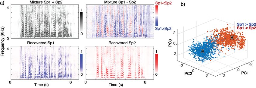
i

Abstract

In this work, we investigate the applicability of the Online Deep Attractor Network
(ODANet) for real-time speech separation on an embedded system with limited pro-
cessing resources. To optimize the ODANet for a resource constrained environment, we
extensively evaluate two different reduction methods. First, we present a detailed anal-
ysis of complexity reduction via hyper-parameter tuning of the ODANet and second,
we introduce a compression method for long short-term memory (LSTM) layers to the
ODANet architecture. While our results suggest that real-time capability is possible for a
desktop computer with these methods, it is not achievable for an embedded device like
the NVIDIA Jetson Nano while maintaining an acceptable separation performance. In
further findings, we show that the utilized compression method for LSTMs is superior
to hyper-parameter tuning in terms of finding a good trade-off between low processing
time and separation performance. Furthermore, we want to highlight that this work is
the first to our knowledge to give an extensive description of a singular value decompo-
sition based compression method for LSTMs including an open-source implementation
available at https://github.com/sp-uhh/compressed-lstm .
ii
Contents                                            iii

Contents

1. Introduction                                                                                  1

2. Related Work                                                                                  5
   2.1. Speech Separation Algorithms . . . . . . . . . . . . . . . . . . . . . . . . . .         5
   2.2. Compression Methods for Neural Networks . . . . . . . . . . . . . . . . .                7
   2.3. Signal Processing with Neural Networks on Embedded Systems . . . . . .                   8

3. Methods                                                                                      11
   3.1. Utilized Methods . . . . . . . . . . . . . . . . . . . . . . . . . . . . . . . . .      11
        3.1.1. Deep Attractor Network (DANet) . . . . . . . . . . . . . . . . . . .             11
        3.1.2. Anchored Deep Attractor Network (ADANet) . . . . . . . . . . . .                 15
        3.1.3. Online Deep Attractor Network (ODANet) . . . . . . . . . . . . . .               18
        3.1.4. Compressed Long Short-term Memory (CLSTM) . . . . . . . . . . .                  21
   3.2. Proposed Methods . . . . . . . . . . . . . . . . . . . . . . . . . . . . . . . .        25
        3.2.1. Sphere Anchor Point Initialization . . . . . . . . . . . . . . . . . . .         25
        3.2.2. Compressed Online Deep Attractor Network (CODANet) . . . . .                     28

4. Evaluation                                                                                   31
   4.1. Experimental Setup . . . . . . . . . . . . . . . . . . . . . . . . . . . . . . . .      31
   4.2. Evaluation Methods . . . . . . . . . . . . . . . . . . . . . . . . . . . . . . .        33
        4.2.1. Scale-invariant Source to Noise Ratio (SI-SNR) . . . . . . . . . . . .           33
        4.2.2. Source-to-Distortion Ratio (SDR) . . . . . . . . . . . . . . . . . . . .         33
        4.2.3. Measurement of Processing Time per Frame . . . . . . . . . . . . .               34
   4.3. Results . . . . . . . . . . . . . . . . . . . . . . . . . . . . . . . . . . . . . . .   35
        4.3.1. Anchor Point Initialization Methods . . . . . . . . . . . . . . . . . .          35
        4.3.2. Impact of Optimizer and Number of LSTM Units on ADANet . . .                     39
        4.3.3. Hyper-parameter Tuning of ODANet . . . . . . . . . . . . . . . . .               40
        4.3.4. Run-time Optimization with Compression . . . . . . . . . . . . . .               42
        4.3.5. Hardware Related Run-time and Real-time Capability . . . . . . .                 44
        4.3.6. Additional Findings . . . . . . . . . . . . . . . . . . . . . . . . . . .        47

5. Discussion                                                                                   51

6. Conclusion                                                                                   55
iv Contents
Bibliography 57
A. Appendix 61
A.1. Compressed LSTM Equations . . . . . . . . . . . . . . . . . . . . . . . . . . 62
A.2. ADANet Architecture Figure Adapted for the First Frame of the ODANet 63
A.3. Fixed Parameters for Hyper-parameter Tuning . . . . . . . . . . . . . . . . 64
A.4. SI-SNR over Processing Time per Frame Including ODANet with 6 Anchors 64
A.5. Processing Time per Frame of ODANet . . . . . . . . . . . . . . . . . . . . 66
A.6. Processing Time per Frame of CODANet . . . . . . . . . . . . . . . . . . . 72Contents v
Acronyms
ADAM Adaptive Moment Estimation
ADANet Anchored Deep Attractor Network
AECNN Auto-Encoder Convolutional Neural Network
BLSTM bidirectional long short-term memory
CLSTM compressed long short-term memory
CNN convolutional neural network
CODANet Compressed Online Deep Attractor Network
CPU central processing unit
DANet Deep Attractor Network
dB decibel
DNN deep neural network
DPCL Deep Clustering
EM expectation maximisation
FFT fast Fourier transform
FP16 16 bit floating point
GFLOPS giga floating point operations per second
GPU graphics processing unit
IBM ideal binary mask
IFFT inverse fast Fourier transform
IRM ideal ratio mask
ISTFT inverse short-time Fourier transform
LPDDR low-power double data rate synchronous dynamic random ac-
cess memory
LSTM long short-term memory
LVCSR large vocabulary conversational speech recognition
MB megabyte
ML machine learning
MSE mean squared error
NN neural network
ODANet Online Deep Attractor Network
PC personal computer
PESQ perceptual evaluation of speech quality score
PIT Permutation Invariant Trainingvi Contents
RMSprop Root Mean Square Propagation
RNN recurrent neural network
SAR sources-to-artifacts ratio
SDR source-to-distortion ratio
SI-SNR scale-invariant source-to-noise ratio
SIR source-to-interferences ratio
SNR sources-to-noise ratio
STFT short-time Fourier transform
SVD singular value decomposition
TASNet Time-domain Audio Separation Network
uPIT utterance-level Permutation Invariant Training
WER word error rate
WFM ’wiener-filter’ like mask
WSJ0 Wall Street JournalList of Figures vii
List of Figures
1.1. Illustration of speech separation system. . . . . . . . . . . . . . . . . . . . . 2
1.2. Spectrograms of mixture, mask, and separated speaker 1 and speaker 2 . . 3
3.1. DANet architecture (training). . . . . . . . . . . . . . . . . . . . . . . . . . . 12
3.2. DANet architecture (inference). . . . . . . . . . . . . . . . . . . . . . . . . . 14
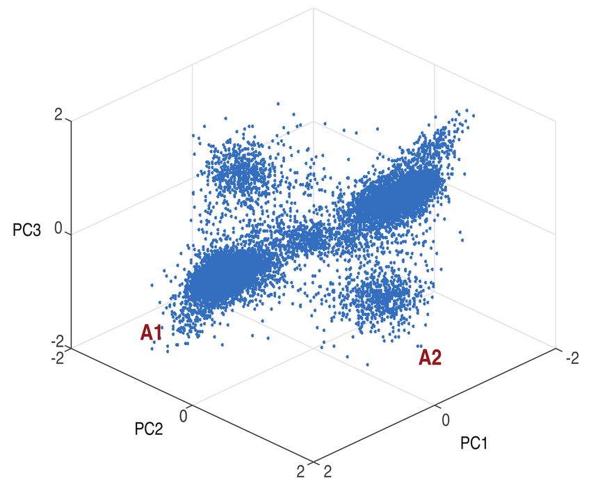
3.3. PCA of attractor points from 10.000 utterances. . . . . . . . . . . . . . . . . 15
3.4. ADANet architecture. . . . . . . . . . . . . . . . . . . . . . . . . . . . . . . . 16
3.5. ODANet architecture (following frames t > 1) . . . . . . . . . . . . . . . . 20
3.6. General RNN and its compressed version. . . . . . . . . . . . . . . . . . . . 22
3.7. The LSTM Cell and its compressed version . . . . . . . . . . . . . . . . . . 24
3.8. Proposed anchor point initialization methods . . . . . . . . . . . . . . . . . 26
3.9. PCA of anchor point movement during training . . . . . . . . . . . . . . . 27
4.1. Illustration of starget as the orthogonal projection of ŝ onto s and enoise as
the difference between ŝ and starget . . . . . . . . . . . . . . . . . . . . . . . . 33
4.2. Discrepancy between validation loss and validation SI-SNR . . . . . . . . 38
4.3. Validation loss of experiment 2.3 with learning rate reduction after epoch
14 from 0.0001 to 0.00005 and after epoch 20 to 0.000025. . . . . . . . . . . 40
4.4. SI-SNR over processing time per frame for ODANet with 4 anchor points
and CODANet . . . . . . . . . . . . . . . . . . . . . . . . . . . . . . . . . . . 43
4.5. Histogram of processing time per frame for CODANet on the PC . . . . . 46
4.6. Histogram of processing time per frame for CODANet on the NVIDIA
Jetson Nano . . . . . . . . . . . . . . . . . . . . . . . . . . . . . . . . . . . . 47
4.7. Validation loss of ADANet experiment with meta-frame size 100 . . . . . 48
4.8. SI-SNR for curriculum training of CODANet . . . . . . . . . . . . . . . . . 48
4.9. SI-SNR over processing time per frame for ODANet 4 LSTM layers and 3
LSTM layers and CODANet . . . . . . . . . . . . . . . . . . . . . . . . . . . 49
A.2. ODANet architecture (first frame t = 1) . . . . . . . . . . . . . . . . . . . . 63
A.3. SI-SNR over processing time per frame for ODANet with 4 and 6 anchor
points and CODANet . . . . . . . . . . . . . . . . . . . . . . . . . . . . . . . 64
A.4. Histogram of processing time per frame for ODANet on the PC with only
CPU . . . . . . . . . . . . . . . . . . . . . . . . . . . . . . . . . . . . . . . . . 70
A.5. Histogram of processing time per frame for ODANet on the PC with GPU 70viii List of Figures
A.6. Histogram of processing time per frame for ODANet on the NVIDIA Jet-
son Nano with only CPU . . . . . . . . . . . . . . . . . . . . . . . . . . . . . 71
A.7. Histogram of processing time per frame for ODANet on the NVIDIA Jet-
son Nano with GPU . . . . . . . . . . . . . . . . . . . . . . . . . . . . . . . . 71
A.8. Histogram of processing time per frame for CODANet on the PC with GPU 73
A.9. Histogram of processing time per frame for CODANet on the NVIDIA
Jetson Nano with GPU . . . . . . . . . . . . . . . . . . . . . . . . . . . . . . 74List of Tables ix
List of Tables
4.1. Preprocessing parameters . . . . . . . . . . . . . . . . . . . . . . . . . . . . 32
4.2. Fixed parameters of first experiment series evaluating the anchor point
initialization methods. . . . . . . . . . . . . . . . . . . . . . . . . . . . . . . 36
4.3. Preliminary experimental results for the different anchor point initializa-
tion methods. . . . . . . . . . . . . . . . . . . . . . . . . . . . . . . . . . . . 37
4.4. Final experimental results for the different anchor point initialization meth-
ods. . . . . . . . . . . . . . . . . . . . . . . . . . . . . . . . . . . . . . . . . . 38
4.5. Experimental results of evaluation of different optimizer settings and num-
ber of units per direction in LSTM of the ADANet. . . . . . . . . . . . . . . 39
4.6. Results of hyper-parameter tuning. . . . . . . . . . . . . . . . . . . . . . . . 41
4.7. Results of Compressed Online Deep Attractor Network. . . . . . . . . . . 42
4.8. Rank for each layer of the CODANet with different compression threshold. 43
4.9. Mean processing time per frame in ms of CODANet on NVIDIA Jetson
Nano and PC . . . . . . . . . . . . . . . . . . . . . . . . . . . . . . . . . . . 45
4.10. Percentage of frames of the CODANet for which the processing time is
larger than the hop size of 8 ms. . . . . . . . . . . . . . . . . . . . . . . . . . 46
5.1. Comparison with other methods on WSJ0-2mix dataset. . . . . . . . . . . . 52
A.1. Fixed parameters for hyper-parameter tuning experiments. . . . . . . . . . 64
A.2. Processing time per frame of ODANet on PC using only the CPU with the
Keras LSTM implementation 1 . . . . . . . . . . . . . . . . . . . . . . . . . 66
A.3. Processing time per frame of ODANet on PC using only the CPU with the
Keras LSTM implementation 2 . . . . . . . . . . . . . . . . . . . . . . . . . 66
A.4. Processing time per frame of ODANet on PC using the GPU with the Keras
LSTM implementation 1 . . . . . . . . . . . . . . . . . . . . . . . . . . . . . 67
A.5. Processing time per frame of ODANet on PC using the GPU with the Keras
LSTM implementation 2 . . . . . . . . . . . . . . . . . . . . . . . . . . . . . 67
A.6. Processing time per frame of ODANet on NVIDIA Jetson Nano using only
the CPU with the Keras LSTM implementation 1 . . . . . . . . . . . . . . . 68
A.7. Processing time per frame of ODANet on NVIDIA Jetson Nano using only
the CPU with the Keras LSTM implementation 2 . . . . . . . . . . . . . . . 68
A.8. Processing time per frame of ODANet on NVIDIA Jetson Nano using the
GPU with the Keras LSTM implementation 1 . . . . . . . . . . . . . . . . . 69x List of Tables
A.9. Processing time per frame of ODANet on NVIDIA Jetson Nano using the
GPU with the Keras LSTM implementation 2 . . . . . . . . . . . . . . . . . 69
A.10.Mean processing time per frame in ms of CODANet . . . . . . . . . . . . . 72
A.11.Variance of processing time per frame of CODANet . . . . . . . . . . . . . 72
A.12.Maximum processing time per frame in ms of CODANet . . . . . . . . . . 73xi
List of Symbols
Symbol Description Dimension
ai Attractor point for speaker i R1×K
at−1,i Attractor point for speaker i at time t − 1 R1×K
Ap Attractor points for combination p (ADANet) RC × K
l
bl Bias of layer l R1× N
bf Training parameter of ODANet’s dynamic weighting R1×K
bg Training parameter of ODANet’s dynamic weighting R1×K
C Number of Speakers N
C Cost function
D Distance between embedding points and attractor points RC× FT
(DANet)
di Distance between embedding points and the attractor point R1× FT
of speaker i
Dp Distance between embedding points and anchor point com- RC× FT
bination p (ADANet)
E Embedding RK× FT
enoise Error signal in time domain for SI-SNR RT
eartif Artifacts error signal in time domain for SDR RT
einterf Interference error signal in time domain caused by e.g. other RT
speakers for SDR
∗
enoise Noise error signal in time domain caused by sensor noise for RT
SDR
f Frequency index {1, 2, . . . , F }xii
Symbol Description Dimension
F Number of frequency bins N
Γp Similarity matrix containing the pairwise similarity between RC × C
the attractor points in the combination p
Γ pi,j Element in row i and column j of similarity matrix Γ p R
γp Maximal pairwise similarity between the attractor points in R
the combination p
l
hlt Output of the l-th layer R1× N
l
helt Projected/compressed output of the l-th layer R1×r
j Anchor point index {1, 2, . . . N }
Jf Training parameter of ODANet’s dynamic weighting RK × K
Jg Training parameter of ODANet’s dynamic weighting RK × K
K Embedding dimension N
l Layer index N
L Loss function
λ Compression threshold [0, 1]
M Masks assign each time-frequency point to the sources in [0, 1]C× FT
proportion to its share in the mixture
M
c Estimated masks [0, 1]C× FT
m
bi Estimated mask for speaker i [0, 1]1× FT
µ Mean of K-dimensional normal distribution RK
N Number of Anchor points N
Nl Number of units in layer l N
NK K-dimensional normal distribution
o Number of operation of a general RNN N
õ Number of operation of a compressed RNN in general N
o∗ Number of operation of a general LSTM Nxiii
Symbol Description Dimension
õ ∗ Number of operation of a compressed LSTM in general N
ψj Anchor point number j R1×K
Ψp Anchor point combination p RC × K
p Anchor point combination index {1, 2, . . . ( N
C )}
fl Σ l
Pl Projection matrix Pl = U fl
h h R N ×r l
rl Rank of layer l N
si ( t ) True speech signal function of speaker i in time-domain R→R
s True speech signal array of speaker i in time-domain RT
ŝ Estimated speech signal array of speaker i in time-domain RT
starget Orthogonal projection of ŝ onto s RT
Si ( f , t ) True complex spectrogram function of speaker i R2 → C
Si True complex spectrogram matrix of speaker i C1× FT
Sbi Estimated complex spectrogram matrix of speaker i C1× FT
Si ( f , t ) True magnitude spectrogram function of speaker i R2 → R
Si True magnitude spectrogram matrix of speaker i R1× FT
l l
Σlh SVD diagonal matrix containing singular values of Wlh RN ×N
Σ
fl
h Truncated SVD diagonal matrix containing the largest rl sin- Rr l × r l
gular values of Wlh
Σ Covariance matrix of K-dimensional normal distribution RK × K
σjl j-th singular value of SDV with σ1l ≥ σ2l ≥ . . . ≥ σN
l
l R
t Time index {1, 2, . . . , T }
T Number of time frames / samples N
τ Context window size (ODANet) N
l l
Ulh SVD matrix containing left-singular vectors of Wlh RN ×N
l
fl
U h Truncated SVD matrix containing the first rl left-singular R N ×r l
vectors of Wlhxiv
Symbol Description Dimension
Uf Training parameter of ODANet’s dynamic weighting R F ×K
Ug Training parameter of ODANet’s dynamic weighting R F ×K
l l
Vlh SVD Matrix containing right-singular vectors of Wlh RN ×N
l
fl
V h Truncated SVD matrix containing the first rl right-singular Rr l × N
vectors of Wlh
Wlx Kernal of layer l R Nl −1 × Nl
l
Wix Kernal of LSTM input gate (layer l) R Nl −1 × Nl
Wlox Kernal of LSTM output gate (layer l) R Nl −1 × Nl
Wlf x Kernal of LSTM forget gate (layer l) R Nl −1 × Nl
Wlcx Kernal of LSTM cell (layer l) R Nl −1 × Nl
W̄lx Combined kernel of LSTM (layer l) R Nl −1 ×4Nl
Wlh Recurrent kernal of layer l R Nl × Nl
l
Wih Recurrent kernal of LSTM input gate (layer l) R Nl × Nl
Wloh Recurrent kernal of LSTM output gate (layer l) R Nl × Nl
Wlf h Recurrent kernal of LSTM forget gate (layer l) R Nl × Nl
Wlch Recurrent kernal of LSTM cell (layer l) R Nl × Nl
W̄lh Combined recurrent kernel of LSTM (layer l) R Nl ×4Nl
Wf Training parameter of ODANet’s dynamic weighting R N4 ×K
Wg Training parameter of ODANet’s dynamic weighting R N4 ×K
x (t) Mixture signal function in time-domain R→R
X ( f , t) Complex mixture spectrogram function R2 → C
X Complex mixture spectrogram matrix C1× FT
X ( f , t) Magnitude mixture spectrogram function R2 → R
X Magnitude mixture spectrogram matix R1× FT
Y True source assignment [0, 1]C× FT
Ŷ Estimated source assignment [0, 1]C× FTxv
Symbol Description Dimension
ŷi Estimated source assignment for speaker i [0, 1]1× FT
Ŷ p Estimated source assignment for anchor point combination [0, 1]C× FT
p
l
Zlh Recurrent kernal back-projection matrix of layer l Rr l × N
Zlx+1 Kernal back-projection matrix of layer l + 1 Rrl × Nl +1
Z̄lx+1 Combined back-projection kernel of LSTM (layer l) Rrl ×4Nl +1
Z̄lh Combined back-projection kernel of LSTM (layer l) Rrl ×4Nlxvi
1

1. Introduction

In real-world speech signal processing applications we often encounter situations where
multiple speakers are active in the signal at the same time, but we are actually interested
in the speech source signal of one or multiple speakers in the mixture. For this so-called
problem of speech separation, great advances have been made by the research commu-
nity in recent years using neural networks (NNs). Still, real-time processing with NNs
requires a lot of computational resources, and so far there is little research like [1] con-
sidering the deployment of speech separation algorithms based on NNs on embedded
devices like mobile phones or hearing aids with limited resources available. In this re-
search work, we strive to close this gap by optimizing the Online Deep Attractor Network
(ODANet) [2] for real-time speech separation on an embedded system through hyper-
parameter tuning and compression with a low-rank matrix factorization technique for
NNs.
  Application fields of the speech separation are for instance automatic meeting tran-
scription or multi-party human-machine interactions for example with speech assistants
[3]. In these application areas it is currently common practice that the audio signals are
sent to a cloud computer and processed there. However, there is a growing interest in
processing the audio signal on mobile devices without the need for an internet connec-
tion and sending the audio data to a cloud computer, which can strongly increase the
latency [4]. Hearing aids are another conceivable field of application for speech separa-
tion algorithms where a short processing time is crucial and the available processing and
memory resources are very limited.
  Mathematically the speech separation problem is defined as separating C speech source
signals si (t) in a mixture
                                                   C
                                      x (t) =     ∑ si ( t )                            (1.1)
                                                  i =1

as shown in the left part of figure 1.1, which illustrates a general speech separation system
for two speakers. Many early NN-based approaches to the speech separation problem
like Deep Clustering (DPCL) [5], Permutation Invariant Training (PIT) [3], or the Deep
Attractor Network (DANet) [2, 6, 7] apply a short-time Fourier transform (STFT) on the
time-domain mixture signal x (t) and solve the speech separation problem in the time-
frequency domain, where the result of the STFT is the complex mixture spectrogram

                                                   C
                                   X ( f , t) =   ∑ Si (t, f )                          (1.2)
                                                  i =1
2 1. Introduction
Speech
Separation
System
Figure 1.1.: Speaker 1 and speaker 2 speaking into the same microphone, which records
the mixture x of the two overlapping signals (s1 and s2 ). The goal of the
speech separation system is to estimate the original speech signals of speakers
1 and 2. (Icons from flaticon.com)
which is the sum of the complex speech source spectrograms Si (t, f ). DPCL, PIT, and the
DANet solve the speech separation problem by generating masks M for the magnitude
mixture spectrogram
X ( f , t) = |X ( f , t)|. (1.3)
For each speaker i the mask mi indicates the affiliation of each time-frequency bin X ( f , t)
in the mixture spectrogram to the speaker i [7]. The goal is to estimate the ideal binary
mask (IBM), the ideal ratio mask (IRM), or the ’wiener-filter’ like mask (WFM) which are
defined as
IBMi, f t = δ(|Si, f t | > |S j, f t |) ∀ j 6= i (1.4)
|Si, f t |
IRMi, f t = (1.5)
∑Cj=1 |S j, f t |
|Si, f t |2
WFMi, f t = (1.6)
∑Cj=1 |S j, f t |2
where Si ∈ R1× FT is the matrix containing the magnitude spectrogram of speaker i and
δ( x ) = 1 if the expression x is true and δ( x ) = 0 if the expression x is false [7]. F and T are
the number of frequency bins and the number of time frames of the STFT respectively.
The source spectrograms Si ∈ C1× FT are estimated as
Sbi = X m
bi (1.7)
where b i is the estimated mask for speaker i and
is the element-wise multiplication, m
X ∈ C1× FT is the complex spectrogram.
Figure 1.1 illustrates the speech separation problem for two speakers and Figure 1.2
shows how a mask can be applied to the mixture in the time-frequency domain to sepa-
rate two speakers.
The discussed time-frequency domain approaches [2, 3, 5–7] use deep neural networks
(DNNs), which are NN with an input layer, an output layer and at least one hidden layer3
Figure 1.2.: Spectrograms of mixture (top left), mask (top right), and separated speaker 1
(bottom left) and speaker 2 (bottom right). Figure from [6].
in between. More particularly they use long short-term memory (LSTM) layers, which
are recurrent neural network (RNN) layers. In RNNs the individual network cells have
recurrent connections, which means each cells has a connection to itself with a time delay.
Because of its recurrent connections and further mechanisms LSTMs are well suited for
NN learning problems where the input has a meaningful time dimension [8], which is
the case for speech signals.
For real-time processing it is required that the used system is causal, which means the
system should only use information from current and past time steps and not look at
future time steps when processing the current time step [9]. Furthermore, the latency
between the audio input and the processed audio output should not be larger than 30 ms
[10]. In this work, we aim for processing times below 8 ms per time frame, which is equal
the hop size we use in the STFT. A NN with LSTMs can only be causal if unidirectional
LSTMs are used in the NNs. However, most of the mentioned systems use bidirectional
long short-term memory (BLSTM) and processes the audio data offline as a non-causal
system. Even if unidirectional LSTMs are used, most of the networks [3, 5–7] process the
time-frequency domain data not frame by frame but require meta-frames, which makes
them non-causal systems.
That is why in this work we try to optimize the ODANet by Han et al. [2], a causal
system, for real-time processing on an embedded system like the NVIDIA Jetson Nano.
For this work we have chosen the NVIDIA Jetson Nano as the test system because this
single-board computer has a similar form factor as the Raspberry Pi and is additionally
equipped with a GPU [11]. To optimize the ODANet for embedded systems we try to
reduce the number of weights especially in the LSTM layers. For this we investigate
two methods, firstly hyper-parameter tuning and secondly compressing the LSTMs with
the compression method proposed by Prabhavalkar et al. [4] based on low-rank matrix
factorization.4 1. Introduction
Our findings suggest that the compression method by Prabhavalkar et al. is better
suited for finding a good trade-off between low processing time and speech separation
performance. By reducing the weights of the ODANet, among other things through the
introduction of the Compressed Online Deep Attractor Network (CODANet), our work
improves the real-time capability of ODANet on embedded systems. However, real-time
speech separation on the selected embedded system, the NVIDIA Jetson Nano, is not
achieved in this work.
The rest of this work is structured as follows. In chapter 2 we present related speech
separation algorithms based on NNs, analyze different compression method for NNs,
and look at related work that also aimed to optimize signal processing NNs for em-
bedded systems. In the methods chapter 3 we explain the ODANet and its evolution
from the DANet over the Anchored Deep Attractor Network (ADANet) in detail. Fur-
thermore, we describe the used compression method by Prabhavalkar et al. [4] and the
resulting compressed long short-term memorys (CLSTMs). Then we introduce the CO-
DANet as well as an optimized way to initialize the anchor points in the ADANet, which
is also used in the ODANet and CODANet. In chapter 4 we present the experimental
setup used to train our NN implementations, the methods we used to evaluate the ex-
periments, followed by the experimental results. Finally, we discuss the results in chapter
5 and conclude the work in chapter 6.5
2. Related Work
In this chapter, we first briefly describe DNN-based single-channel speech separation
algorithms related to the DANet. Second, we look at the different methods for the com-
pression of NNs in general and explain our choice for the compression method of by
Pravhavalkar et al. [4]. In the third part of this chapter, we present related work on the
optimization of NN-based signal processing algorithms for embedded systems with nu-
merical results.
2.1. Speech Separation Algorithms
In recent years there has been great progress in the research on single-channel speech
separation with DNNs. These DNN-based algorithms can be categorized into algorithms
operating in the time-frequency domain and algorithms operating directly in the time
domain. Well known time-frequency domain approaches are (among others) DPCL by
Hershey et al. [5] and PIT by Yu et al. [3].
The DPCL network maps each time-frequency bin into a higher dimensional embed-
ding space E ∈ RK× FT with the training objective to minimize the cost function
CY (E) = kET E − YT Yk2F (2.1)
which calculates the distance in the Frobenius norm k · k F between the true affinity matrix
Y T Y and the estimated affinity matrix E T E. 1 With this cost function the network learns
to map time-frequency bins belonging to the same speaker into similar regions in the
embedding space while separating time-frequency bins belonging to different speakers.
During training, this is achieved using the true source assignments Y, while during in-
ference the network separates the sources by applying k-means in the embedding space,
where the k-means clusters are equivalent to the estimated source assignments.
The DPCL method is further improved by Isik et al. [12] and Wang et al. [13] who
present the DPCL++ and Chimera++ networks, respectively. Wang et al. [14] also present
a low-latency DPCL version by replacing the bidirectional LSTMs with unidirectional
LSTMs and changing the STFT window size from 32 ms to 8 ms. The cluster centers for
k-means are calculated for the first 1.5 seconds of the signal during, which the network
1 The notation from [5] is adapted to match the notation in this work. In [5] the embedding space is
V ∈ RFT ×K in our work the embedding space is E ∈ RK × FT . In [5] the true source assignment is Y ∈ RFT ×C
in our work the true source assignment is Y ∈ RC× FT .6 2. Related Work
is not able to generate any output. Afterwards, these cluster centers are used to generate
the cluster assignments frame by frame for the rest of the utterance. In comparison the
ODANet has a more dynamic way to calculate the cluster centers (attractors) online by
updating them using a exponentially weighted moving average (see section 3.1.3).
PIT by Yu et al. [3] directly generates a mask from the magnitude spectrogram of the
mixture input X using a DNN. This mask is then used to estimate the source signals
Ŝi . Because there is a high probability of a permutation in the output (e.g. Ŝ1 is a good
estimate for S2 and vice versa), which would cause a high error in the training objective,
which is to minimize the mean squared error (MSE) between Ŝi and Si for i = 1, . . . , C,
PIT minimizes the MSE for the permutation with the lowest MSE. Kolbaek et al. present
an advanced version of PIT called utterance-level Permutation Invariant Training (uPIT)
[15], which predicts phase sensitive masks instead of amplitude masks. Furthermore,
the network architecture is improved by using LSTMs instead of non-recurrent DNNs or
convolutional neural networks (CNNs), which are used in PIT and limit the network to
a fixed input and output size. Because of this architecture change, uPIT is able to predict
different input and output sizes and is also causal if unidirectional LSTMs are used.
One limitation of most DNN-based speech separation approaches in the time-frequency
domain is that their performance is limited by the IBM, IRM, or WFM on the magni-
tude spectrogram, while the phase information for each source is taken from the mix-
ture. In contrast, the Time-domain Audio Separation Network (TASNet) by Luo and
Mesgarani [16] shows that time domain approaches can outperform time-frequency do-
main approaches because the former do not have this limitation. In addition to the per-
formance advantages TASNet has also an advantage in the algorithmic latency because
it does not require an STFT and works directly on the time domain signal on segments as
short as 5 ms [16].
The TASNet uses an encoder-decoder framework and performs the speech separation
by masking the encoder outputs, which are non-negative weights of the base signals
contained in the audio segment to be separated [16]. The NN architecture of TASNet
is further improved in [17–19]. In the NNs described in these papers, the base signals
for the encoder and decoder are learned by the networks as trainable parameters. Ditter
and Gerkmann [20] show that using a deterministic multi-phase gammatone filterbank
instead of the learned base signals in the encoder-decoder framework further improves
the performance. Other recent time-domain approaches to the speech separation problem
are Wave-U-Net [21], FurcaNeXt [22], SepFormer [23], and Wavesplit [24].
Despite the advantages of the time-domain approaches, we focus on the ODANet,
which operates in the time-frequency domain, because the ODANet is a causal systems
with a relatively small model size (compare table 5.1 on page 52) and because in pre-
liminary work we have successfully implemented a time-frequency domain speech sep-
aration algorithm for real-time processing. Nevertheless, the compression method by
Prabhavalkar et al. [4] can be applied to all DNN-based speech separation algorithms2.2. Compression Methods for Neural Networks 7 using RNNs in particular LSTMs, which is the case for the original TASNet in [16]. In the discussion, chapter 5, we compare our results to the related work mentioned in this section in terms of the performance and the model size. 2.2. Compression Methods for Neural Networks In their survey paper Choudhary et al. [25] summarize several approaches for the com- pression and acceleration of machine learning (ML) models. The four main approaches to compress and accelerate a NN are • pruning, • quantization, • knowledge destillation, • low-rank factorization. The main goal of pruning is to reduce the storage-size of the network. This is achieved by zeroing out network weights that are below a certain threshold or redundant. How- ever, though pruning reduces the number of weights and thereby the model size, pruning does not reduce the number of operations by default. Only if neuron pruning or layer pruning is applied, which removes entire neurons or layers of a DNN, the number of operations is reduced [25]. Quantization of the network weights can lead to a significant size reduction. On the one hand, uniform quantization can also reduce computing time, e.g. quantizing 32- bit weights to 16-bit or 8-bit weights if the hardware efficiently processes 16-bit or 8-bit operations. On the other hand, while a non-uniform quantization can greatly reduce the model size, it cannot reduce the computation time [25]. In knowledge distillation a smaller ’student’ network is trained to generate the outputs of a larger ’teacher’ network when shown the same data. Knowledge distillation works good for classification problems [25]. In low-rank matrix factorization weight matrices W ∈ Rm×n are factorized in to matri- ces P ∈ Rm×r and Z ∈ Rr×n using a singular value decomposition (SVD) so that PZ is the best rank r approximation of W. This reduces the size and the number of operations for a specific matrix from m · n to r · (m + n) [25]. This method is explained in detail in section 3.1.4. We choose low-rank matrix factorization for compressing the ODANet because it is a deterministic method to reduce the size and the number of operations of a NN and because it has been previously applied to RNNs in particular LSTMs by Prabhavalkar et al. for automatic speech recognition [4].
8                                     2. Related Work

2.3. Signal Processing with Neural Networks on Embedded
       Systems

While the previous section presents compression methods for NNs in general, this sec-
tion presents related work on signal processing with neural networks on embedded sys-
tems with numerical results. This work is closely related to our work in the sense that
it also considers the optimization of NN-based speech enhancement systems for embed-
ded systems [26, 27] or compares the processing time of image processing NNs on the
NVIDIA Jetson Nano to the procssing time on a desktop with a graphics processing unit
(GPU) [28].
    In speech enhancement the goal is to retrieve the clean speech signal s(t) from the
signal
                                      x (t) = s(t) + n(t)                                 (2.2)

in which the clean speech signal is distorted with noise n(t). Although speech enhance-
ment and speech separation are related problems, they differ in that in speech separation
several similar speech signals are to be separated from each other, whereas in speech
enhancement exactly one speech signal is to be separated from the noise signal, which
often has slightly different characteristics. Nevertheless, since this work is one of the first
works to optimize a NN-based speech separation system for real-time processing on an
embedded systems, we consult the results from [26, 27] in our discussion.
    Drakopoulos et al. [26] propose the Auto-Encoder Convolutional Neural Network
(AECNN) for real-time speech enhancement on an embedded system, in particular the
Raspberry Pi 3 Model B+. They optimize the AECNN for the embedded system by hyper-
parameter tuning the number of CNN layers and the number of filters in the CNNs.
They report execution times from 42 ms per frame of size 1024 samples at a sampling
rate of 16 kHz for a network with 3 million parameters to 5.7 ms per frame for a net-
work with 0.2 million parameters and a frame size of 128 frames at a sampling rate of
16 kHz. Drakopoulos et al. present the speech enhancement performance in terms of the
perceptual evaluation of speech quality score (PESQ) [29] and the segmental sources-to-
noise ratio (SNR) [26] but do not compare their results to a baseline or any other research.
Among other results Drakopoulos et al. report that their network is 6.5% faster with a
Tensorflow frontend than with a Keras frontend [26].
    In contrast to Drakopoulos et al., who use hyper-parameter tuning for the embed-
ded optimization, Fedorov et al. [27] propose TinyLSTM, which is optimized for embed-
ded speech enhancement on hearing aids by applying pruning and integer quantization.
Their baseline architecture consists of 2 unidirectional LSTM layers with 256 units in
each layer and two fully connected layers with 128 units in each layer. With a total of 0.97
million parameters their baseline is about 12-times smaller than our ODANet baseline,
which has almost 12 million parameters (see equation 3.44 on page 29 for the calculation
of the number of parameters of the ODANet). With pruning and quantization from 32bit
2.3. Signal Processing with Neural Networks on Embedded Systems 9 floating point weights to 8 bit integer weights Fedorov et al. are able to reduce the model size from 3.7 megabyte (MB) to 0.31 MB, while the number of parameters is reduced to 34% of the baseline from 0.97 million to 0.33 million. This size reduction results in a time reduction from 12.52 ms to 4.26 ms per frame on a micro-controller unit hardware. Fedorov et al. are able to achieve this reduction in the model size with only a small re- duction of 4% in the source-to-distortion ratio (SDR) speech enhancement performance on CHiME2 WSJ0 dataset [30]. Last but not least, we would like to mention related work on the NVIDIA Jetson hard- ware. Bianco et al. [28] compare the performance and run-time of image recognition DNNs on a desktop computer with a NVIDIA Titian X Pascal GPU to the performance and run-time of the same DNNs on the NVIDIA Jetson TX1 board, which has 256 GPU cores compared to 128 GPU cores on the NVIDIA Jetson Nano, but other than that com- parable hardware specifications [11,31] (all relevant NVIDIA Jetson Nano hardware spec- ifications are presented in section 4.1 on page 32). Bianco et al. report that the NVIDIA Jetson TX1 takes 5 to 35 times longer than the personal computer (PC) with the NVIDIA Titian X Pascal GPU to process a single image. We use these values as an orientation for our evaluation of the ODANet and the CODANet, which are presented in the next chapter.
10 2. Related Work
11

3. Methods

This chapter introduces the methods we used for our implementation (section 3.1) as well
as our proposal to combine and extend these methods to the Compressed Online Deep
Attractor Network (CODANet) (section 3.2).

3.1. Utilized Methods

In this section, we describe the Deep Attractor Network (DANet) and its evolution from
the first paper [6] over the Anchored Deep Attractor Network (ADANet) [7] to the Online
Deep Attractor Network (ODANet) [2]. For each network we explain the general idea,
the architecture, and implementation details of our implementation that differ from the
original description.
  Furthermore, we present the compression method by Prabhavalkar et al. [4] for RNNs
that jointly compresses the recurrent and non-recurrent weight matrices of RNN layers
with a low-rank matrix factorization and leads to the CLSTM.

3.1.1. Deep Attractor Network (DANet)

To solve the speech separation problem, the DANet by Chen et al. [6] learns to map
time-frequency bins belonging to the same speaker close to the attractor point of that
speaker in the embedding space. Similar to DPCL [5] the idea of the embedding space is
that points belonging to the same speaker are mapped close to each other, while points
belonging to different speakers are supposed to have a large distance1 in the embedding
space. In the DANet this mapping is not the explicit goal but rather are the mapping into
the embedding space and the positions of the attractor points implicitly learned by the
overall training target.
  The idea behind the attractor points is that each attractor point attracts the time-frequency
bins of a specific speaker assigned to it and at the same time repels time-frequency bins
of other speakers. The idea of the attractors is based on the perceptual magnet effect
observed by Kuhl [32]. Kuhl shows that humans can identify prototypes of speech cat-
egories if they are played the prototype sound and variations of it. In one of his experi-
ments for example adults were plaid different variations of the /i/ vowel and asked to
rate the goodness of it. This experiment showed that across all listeners the rating was
similar and the prototype /i/ vowel was always rated best. In further experiments Kuhl
   1 In   DANet the dot product is used as the distance measure.
12                                         3. Methods

shows that these prototypes of sound categories serve as reference mental representations
(reference points) when listening to speech sounds. These reference points are called per-
ceptual magnets. The idea of the DANet can be seen as learning perceptual magnets for
speaker characteristics. In the DANet the perceptual magnets are called attractor points.

                    Estimated Sources

                                                                               DANet
                                                                            (training)

                    Masks

                                                               Attractors
                     Mask Calculation

                                                          Attractor Calculation
                                                                    as
                Embedding                                  ideal cluster centers

                      Fully-connected
                            Layer

                     4 (B)LSTM Layers

                  Magnitude Spectrogram

                 Convert to Absolut Values
                    in dB and Capping

                     Input                              True Source Assignments
                    (T-F Representation)

      Figure 3.1.: DANet architecture (training). Graphic adapted from [7, p. 789].

  In the following we describe the DANet architecture that tries to implement this idea.
Figure 3.1 shows our DANet architecture during training based on [6]. The input to the
network is the complex spectrogram X ∈ C1× FT . This input is converted into the real val-
ued magnitude spectrogram X ∈ R1× FT in decibel (dB). Furthermore, the network cappes
the magnitude spectrogram in dB at −80 dB and 200 dB to avoid large negative and pos-
itive values. The magnitude spectrogram in dB is then mapped into the K-dimensional
3.1. Utilized Methods 13
embedding space E ∈ RK× FT by four LSTM layers and one fully-connected layer.
During training the attractor points A ∈ RC×K are calculated as the ideal cluster centers
of the time-frequency bins belonging to the same speaker
yi E T
ai = i = 1, 2, . . . , C (3.1)
∑ f ,t yi
using the true source assignment Y ∈ RC× FT . The true source assignment can be the IBM,
IRM, or the WFM.
b i ∈ R1× FT for speaker i by
Using the attractor points the DANet estimates the mask m
calculating the distance between the time-frequency bins and the attractor points in the
embedding space
di = ai E i = 1, 2, . . . , C (3.2)
and assigning each time-frequency bin to the source of the attractor point that it is closest
to in the embedding space
b i = H(di )
m i = 1, 2, . . . , C (3.3)
where H(di ) is the softmax or sigmoid function
exp(di, f t )
softmax(di, f t ) =
∑Cj=1 exp(d j, f t )
H(di ) = . (3.4)
sigmoid(di, f t ) =
1
∑Cj=1 (1+exp(−d j, f t )
M ∈ RC× FT the estimated complex source spectrograms
Using the estimated masks c
Sbi ∈ C1×TF for each speaker i are calculated as
Sbi = X m
bi i = 1, 2, . . . , C (3.5)
where is the element-wise multiplication.
The training objective of the DANet is to minimize the MSE loss function
C
1
L=
C·F·T ∑ kSi − Sbi k22 (3.6)
i =1
between the estimated source signals Sbi and the true source signals Sbi .
Because the true source assignments Y are unknown during the inference of the DANet,
the network architecture changes from training to inference. Figure 3.2 shows the DANet
inference architecture. The network architecture from the spectrogram input X to the
embedding E, which contains all trainable parameters, is the same for training and infer-
ence. What changes is the way the attractor points are calculated. During the inference
the k-means clustering algorithm is used to identify clusters of time-frequency bins in the
embedding space and the resulting cluster centers are chosen to be the attractor points.14 3. Methods
Estimated Sources
DANet
(inference)
Masks
Mask Calculation Attractors
k-means cluster
Attractor Calculation
with k-means
Embedding as cluster centers
Fully-connected
Layer
4 (B)LSTM Layers
Magnitude Spectrogram
Convert to Absolut Values
in dB and Capping
Input
(T-F Representation)
Figure 3.2.: DANet architecture (inference). Graphic adapted from [7, p. 789].3.1. Utilized Methods 15
Using these attractor points the estimated binary mask is equivalent to the cluster assign-
ments in k-means.
Our implementation differs from the DANet implementation from Chen et al. [6] in
two ways. First, Chen et al. do not describe capping the magnitude values at −80 dB
and 200 dB. Second, we use the complex spectrograms in the MSE loss function L. In
contrast, Chen et al. do not explicitly mention if they use the complex or real-valued
magnitude spectrogram in the loss function. Furthermore, Chen et al. use the squared
error and not the mean squared error for their loss function. We use the mean squared
error to be able to better interpret the value of the loss function.
The main disadvantages of the DANet are that the architecture differs between training
and inference and that it uses k-means during inference, which is computationally expen-
sive. To overcome these disadvantages Luo et al. propose the Anchored Deep Attractor
Network, which is presented in the next section.
3.1.2. Anchored Deep Attractor Network (ADANet)
Evaluating the experiments of the previously described DANet the authors, Chen, Luo,
and Mesgarani, observed that the attractor points always lie in similar regions as shown
in figure 3.3. Based on this observation, they proposed two further methods to find the
attractor points in addition to k-means in [7].
Figure 3.3.: PCA of attractor points from 10.000 utterances. A1 and A2 highlight regions
of attractor point pairs. Edited graphic from [6, p. 249].
1. Fixed attractor points: The first idea mentioned in [6] and [7] is to use a pair of
fixed attractor points (one attractor point for each speaker). E.g. the cluster centers
of regions A1 in figure 3.3 could be used as the fixed pair of attractor points.
2. Anchor points: The second idea is to use anchor points to get an estimated source
assignment Y,
b which is then used to calculate the attractor points using16 3. Methods
equation 3.1. The position of the anchor points are also learned during the training
of the ADANet. This method can also be seen as reducing the k-means algorithm
to one single expectation maximisation (EM) step with an intelligent initialization
of the cluster centers for the expectation step with the anchor points.
Estimated Sources
Anchored DANet
(training and inference)
Masks
Attractors
Mask Calculation
Attractor Calculation
and selection of
Embedding best attractor combination
Estimated Source Assignments
Fully-connected
Layer
Source Assignment Esitmation
with Anchors
4 (B)LSTM Layers
Magnitude Spectrogram
Convert to Absolut Values
in dB and Capping
Input
(T-F Representation)
Figure 3.4.: ADANet architecture. Graphic adapted from [7, p. 789].
The second idea, which leads to the ADANet is explained in detail in this section.
Figure 3.4 show the architecture of the ADANet. The left part is equivalent to the DANet.
What changes is the way the attractor points are calculated illustrated on the right side
of the figure. The ADANet uses N anchor points ψ j ∈ R1×K to estimate the source
assignment where N is chosen to be greater than or equal to the number of speaker C.
Each anchor point functions as a reference point for a probable attractor point position.3.1. Utilized Methods 17
The anchor points are initialized randomly and the probable anchor point positions are
learned during the training of the network, which strongly correlate with the attractor
point positions.
For all ( N
C ) combinations of the anchor points the resulting estimated source assign-
ment is calculated in the following way. Let Ψ p ∈ RC×K be the p-th combination of C
anchor points with p = 1, 2, . . . ( N
C ). (E.g. Ψ1 = [ ψ1 ψ2 ] ) For each combination p the
T
distance between the time-frequency points and the anchor points of this combination is
calculated similar to equation 3.2 as
N
D p = Ψ p E, p = 1, 2, . . . . (3.7)
C
Afterwards, the estimated source assignment for the combination p is calculated as
Ŷ p = so f tmax (D p ). (3.8)
In the following, equation 3.1 is used to calculate the attractor points A p ∈ RC×K for
each possible source assignment p in the ( N
C ) combinations resulting in the same number
of possible attractor point combinations. Now the best attractor point combination is
selected, which is the combination of attractor points where the distance between the
two closest attractor points in the combination is maximal. This combination is found
using the following equations.
A similarity matrix Γ p ∈ RC×C that contains the pairwise similarity between the attrac-
tor points in the combination p is calculated as
Γ p = A p A Tp (3.9)
where A p contains the row vectors of the attractor points in the combination with the
index p. For example for 3 speakers (C = 3) A1 would have the following structure
· · · a1 · · ·
∈ R3 × K .
A1 =
· · · a2 · · ·
· · · a3 · · ·
This results in the following similarity matrix
h a1 , a1 i h a1 , a2 i h a1 , a3 i
Γ p =1
=
h a2 , a1 i h a2 , a2 i h a2 , a3 i
h a3 , a1 i h a3 , a2 i h a3 , a3 i
where hai , a j i denotes the dot product between attractor ai and a j . This dot product mea-
sures the similarity between the two attractor points and is maximal if ai and a j are iden-
tical. The absolute value of the dot product is minimal if the two vectors ai and a j are
orthogonal. The dot product reaches its minimum (a negative value) if the two vectors ai18 3. Methods
and a j are pointing in opposite directions from the origin.
The maximum value of the non-diagonal values of Γ p is selected as
γ p = max{Γ pi,j }, i 6= j (3.10)
which represents the attractor point pair in the combination p with the largest similarity.
Finally, the combination of attractor points A p , for which the largest in-set similarity
γ p between the two most similar attractor points is minimal, is selected as
N
A = argmin{γ p }, p = 1, 2, . . . , (3.11)
Ap C
which is the combination of attractor points, for which the distance between the two
closest attractor points in the combination is maximal. Now this best attractor point
combination A is used to calculate the estimated masks and estimated signal sources,
which is done analogously to the DANet.
The ADANet eliminates the disadvantages of the DANet by introducing anchor points,
which allow the architecture to be the same for training and inference and reduce k-
means clustering to one EM step, which is directly integrated in the network.
One difference between our ADANet implementation and the implementation by Lue
et al., is that Luo et al. use a salient weight threshold keeping 90% of the salient time-
frequency bins for the attractor calculation while the other 10% are not taken into account
for the attractor calculation (equation 3.1). We do not investigate this difference because it
only improves the scale-invariant source-to-noise ratio (SI-SNR) by less than 5% [7] and it
is not clear how to implement this threshold in real-time. For example with a fixed salient
weight threshold the results depend on the level of the audio signal. A relative threshold
is more complicate to implement in real-time because it has to be updated using e.g. a
moving average.
In the following section, we describe the ODANet a causal version of the ADANet.
3.1.3. Online Deep Attractor Network (ODANet)
The ODANet by Han et al. [2] has the same network architecture as the ADANet in terms
of the LSTM layers and the dense layer but processes the spectrogram frame by frame.
Because the network architecture including the trainable weights does not change, Han
et al. suggest to use the weights of a previously trained ADANet in the ODANet. What
changes is the way the attractor points are calculated.
For the first frame (t = 1) in the ODANet the attractor points are calculated using the
anchor points just like in the ADANet. Therefore, the ODANet architecture for the first
frame is similar to the ADANet architecture shown in figure 3.4. This figure is adapted
specifically for the first frame of the ODANet in the appendix A.2 by changing the di-
mensions from FT to F indicating that the ODANet processes single frames.3.1. Utilized Methods 19
For every following frame the previous attractor points At−1 are used instead of the
anchor points to estimate the source assignments
Ŷt = softmax(At−1 Et ). (3.12)
Based on this source assignment estimation Ŷt the current attractor point position for
speaker i is estimated equivalent to equation 3.1 as
ŷt,i EtT
ât,i = i = 1, 2, . . . , C. (3.13)
∑ f ŷt,i
To avoid that the attractor points jump around between time frames (e.g. during silence
frames), Han et al. propose to use an exponentially weighted moving average for updat-
ing the position of the attractor points as follows
at,i := αt,i ât,i + (1 − αt,i )at−1,i . (3.14)
Furthermore, they propose two ways to calculate the update coefficient αt,i
1. context-based weighting,
2. dynamic weighting.
In context-based weighting the update coefficient αt,i is calculated as
∑ f ŷt,i
αt,i = t (3.15)
∑ j=t−τ ∑ f ŷ j,i
where τ is the number of time frames taken into the context-window. This means that
if there is a large number of time-frequency bins belonging to speaker i in the current
time frame t compared to the number of time-frequency bins belonging to speaker i in
the previous τ time frames, then the update coefficient αt,i for speaker i at time frame t
is high. With a high update coefficient the current estimate ât,i has a large impact on the
value at,i while the old value at−1,i is discounted stronger.
In the dynamic weighting the update coefficients are learned by the network as
gt,i · ∑ f ŷt,i
αt,i = −1
(3.16)
ft,i · ∑tj= t−τ ∑ f ŷ j,i + gt,i · ∑ f ŷt,i
where gate gt,i and forget-gate ft,i are calculated as
gt,i = σ(hlt= 4
−1 W g + X t U g + a t −1 J g + b g ) (3.17)
ft,i = σ(hlt= 4
−1 W f + X t U f + a t −1 J f + b f ) (3.18)20 3. Methods
−1 ∈ R
where hlt= 4 1× N4 is the output of the fourth LSTM layer with N units at time t − 1,
4
Xt is the magnitude spectrogram at time t, and at−1 is the attractor point for speaker i at
time t − 1. The other parameters Wg , Wf ∈ R N4 ×K , Ug , Uf ∈ RF×K , Jg , Jf ∈ RK×K , and
bg , bf ∈ R1×K are trainable weights.
For this work, we do not implement the dynamic weighting because it only slightly
improves the SDR by 5% according to [2, p. 363, table 1] and it is computationally more
complex than the context based weighting mechanism.
Estimated Sources
Online DANet
(following frames )
Masks
Attractors
Mask Calculation
Attractor Calculation
with context-based weighting
Embedding or dynamic weighting
Fully-connected Estimated Source Assignments
Layer
Source Assignment Esitmation
with previous Attractors
4 LSTM Layers )
Mag. Frame-Spectrogram
Convert to Absolut Values
in dB and Capping
Input-Frame
(F Representation)
Figure 3.5.: ODANet architecture (following frames t > 1). Red lines represent recurrent
connections with time delay. The dashed box with rounded edges represents
a super-process that combines the entire attractor calculation for the follow-
ing frames and the attractor calculation for the for the first-frame, which is
shown in the appendix in figure A.2 on page 63. Graphic adapted from [7, p.
789].3.1. Utilized Methods 21
Figure 3.5 shows the ODANet architecture for the frames following the first frame with
t > 1. The red line from the attractors to the source assignment estimation represents the
recurrent connection required for the source assignment estimation with the attractors
from the previous time step (equation 3.12). Another recurrent connection is required for
calculating the update coefficient in the context-based weighting (equation 3.15). Here
the recurrent connection contains the history of
∑ ŷt,y (3.19)
f
for t in t − τ to t − 1.
The entire attractor calculation for the first frame and the following frames of the
ODANet is implemented in a super-process represented by the dashed box with rounded
edges in figure 3.5 and figure A.2 in the appendix on page 63. This super-process has a
first_frame flag, which is set to zero for the first frame and one for every following
frame. Based on this flag the super-process calculates the attractor points using the an-
chor points (for the first frame) or the previous attractor points for every following frame.
All weights in the ODANet are initialized with weights from a previously trained
ADANet also known as curriculum training [2]. Due to time constrains we use the
weights from the ADANet directly in our ODANet experiments without further train-
ing the ODANet.
3.1.4. Compressed Long Short-term Memory (CLSTM)
In this section, we first present the compression method for RNNs by Prabhavalker et
al. [4] in general. Then we detail how this method can be applied to LSTMs and thus
leads to the CLSTMs.
The compression method by Prabhavalker et al. is a generalization of the method from
Xue et al. [33]. Both methods are low-rank factorization compression methods. In con-
trast to the method by Xue et al. [33], which only compresses the kernel using a SVD,
the method by Prabhavalker et al. [4] jointly optimizes the recurrent kernel and kernel
of the following layer. This is achieved by a low-rank factorization of the recurrent ker-
nel Wlh ∈ R Nl × Nl , splitting it into a projection Pl ∈ R Nl ×rl and a back-projection matrix
Zlh ∈ Rrl × Nl , followed by an adaption of the kernel Wlx+1 ∈ R Nl × Nl +1 of the next layer to
match the projection matrix Pl . 2
This idea is illustrated in figure 3.6. Figure 3.6a shows layer l of a general RNN and
figure 3.6b shows the compressed version. In the compressed version the output hlt ∈
R1× Nl is multiplied with the projection matrix Pl resulting in the projected output h
el ∈
t
R1×rl , which is used in the recurrent part of layer l and passed to the next layer l + 1. In
the following, we explain the calculation of the matrices for the compressed RNN.
2 The superscripts l and l + 1 on the weight matrices are layer indices and not exponentials.You can also read