Panel Econometric Analysis on Mobile Payment Transactions and Traditional Banks Effort toward Financial Accessibility in Sub-Sahara Africa
←
→
Page content transcription
If your browser does not render page correctly, please read the page content below
sustainability

Article
Panel Econometric Analysis on Mobile Payment
Transactions and Traditional Banks Effort toward
Financial Accessibility in Sub-Sahara Africa
Cephas Paa Kwasi Coffie 1,2 , Hongjiang Zhao 1,2, * and Isaac Adjei Mensah 3
 1    School of Management and Economics, University of Electronic Science and Technology of China,
      Chengdu 610054, China; coffiecephas@gmail.com
 2    Center of West African Studies, University of Electronic Science and Technology of China,
      Chengdu 610054, China
 3    Institute of Applied Systems Analysis (IASA), Faculty of Science, Jiangsu University,
      Zhenjiang 212013, China; isaacadjeimensah29@outlook.com
 *    Correspondence: zhaohj@uestc.edu.cn; Tel.: +86-159-8219-3880

 Received: 6 January 2020; Accepted: 18 January 2020; Published: 24 January 2020

 Abstract: The financial landscape of sub-Sahara Africa is undergoing major changes due to the advent
 of FinTech, which has seen mobile payments boom in the region. This paper examines the salient role
 of mobile payments in traditional banks’ drive toward financial accessibility in sub-Sahara Africa by
 using panel econometric approaches that consider the issues of independencies among cross-sectional
 residuals. Using data from the World Development Index (WDI) 2011–2017 on 11 countries in
 the region, empirical results from cross-sectional dependence (CD) tests, panel unit root test,
 panel cointegration test, and the fully modified ordinary least squares (FMOLS) approach indicates
 that (i) the panel time series data are cross-sectionally independent, (ii) the variables have the same
 order of integration and are cointegrated, and (iii) growth in mobile payment transactions had
 a significant positive relationship with formal account ownership, the number of ATMs, and number
 of new bank branches in the long-run. The paper therefore confirms that the institutional structure
 of traditional banks that makes them competitive, irrespective of emerging disruptive technologies,
 has stimulated overall financial accessibility in the region leading to overall sustainable growth in
 the financial sector. We conclude the paper with feasible policy suggestions.

 Keywords: mobile payment; traditional banks; financial access; FinTech; sub-Sahara Africa

1. Introduction
      The union between technology and finance has significantly reshaped the global financial
landscape in the past decade due to the growing diffusion rate of financial technology–related products
and services [1]. FinTech is an industry of companies using technology to make financial systems
and the delivery of financial products and services more efficient [2]. Although FinTech has a constantly
growing ecosystem with a wide segment of offerings in financing, asset management, and payments,
the flagship FinTech offering in sub-Sahara Africa is mobile payment [2]. While crowdfunding contracts,
Initial coin offerings (ICOs), and blockchain technology seems to rely on relatively complex technologies,
mobile payments operate a simple, convenient, and cost effective technology for the delivery of financial
products and services. The simplicity of the technology continually drives the high diffusion rate across
sub-Sahara Africa, thus attracting curiosity from policy makers and researchers alike [2]. Globally, there
are an estimated 866 million registered customers and an average of 1.3 billion transactions per day from
the industry. Further, statistics indicate that sub-Sahara Africa alone holds over 50% share of the total
global customer base, and with the mobile phone penetration expected to grow up to 500 million

Sustainability 2020, 12, 895; doi:10.3390/su12030895                       www.mdpi.com/journal/sustainability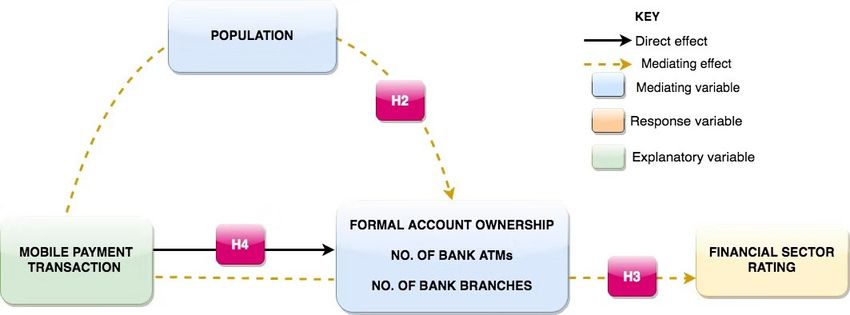
Sustainability 2020, 12, 895                                                                          2 of 20

subscribers by the year 2020, the region has huge potential in this domain of FinTech (the Mobile
Economy Sub-Saharan Africa 2018 report). The introduction of mobile payment in sub-Sahara Africa
championed mainly by Telecos has been hailed as one of the grand financial innovations to improve
the status of financial inclusion in the region as a result of the failed efforts of traditional banks to
financially include many in preceding decades [3,4].
      The past decade witnessed high profile studies on the potential impact of mobile payments on
financial inclusion and reducing poverty in the region [2,3,5], with seemingly little attention given to
the efforts of traditional banks to improve financial accessibility beyond collaborations with FinTech
operators in the form of acquisition, alliance, incubation, and joint ventures [6–8]. This continues to
divide opinions on the relevance of traditional banks (aside from these collaborations). It is spot-on
to say that the emergence of new innovations sometimes threatens to eliminate the existing systems,
especially if the offering is better in terms of ease, convenience, and cost of usage [9]. An example of such
innovation is the blockchain technology that successfully eliminates intermediation (banks, financial
institutions, regulators) with regard to cryptocurrency trade and the execution of smart contracts [10,11].
Nonetheless, traditional banks are known for their tough resistance to change due to their regulations
and structure of operations [12], and we estimate that, although banks in sub-Sahara Africa choose to
collaborate with FinTech operators to benefit from the emerging technologies in the industry, they would
further compete with FinTech operators the old fashion way by expanding their physical infrastructures,
like the number of automated teller machines (ATMs) and the number of branches, to improve overall
accessibility. Consequently, our study analyses the relationship between the growth in mobile payment
transactions and traditional banks’ efforts to expand their infrastructure (formal account ownership,
number of ATMs, and number of bank branches) toward greater financial accessibility.
      While many studies emphasise the importance of mobile payments in poverty reduction, financial
inclusion, and the competitive threats posed by mobile payments operators to traditional banks
in the region, we provide a different perspective ignored by intensive research as we look beyond
collaborations and threats to probe the relationship between the growth in mobile payments transactions
and traditional banks’ efforts to remain competitive with their existing offerings. The study is significant
to FinTech practitioners, researchers, and other stakeholders because (i) it provides deeper intuition
into the dynamism of financial accessibility trends in sub-Sahara Africa by looking beyond current
traditional banks–FinTech collaborations to assess how competition forces these banks to actively
invest in traditional physical infrastructures to make their services accessible and (ii) to distinguish our
study from existing literature, we use Panel data cases from 11 countries and apply recently developed
econometric methods that are capable of producing robust results to serve as the starting point for
future studies within the domain.
      The remainder of this paper is scheduled as follows: the review of related literature and hypothesis
formulation, the detail explanation of the research methodology employed for the study and model
development in detail, data analysis and interpretation, study results, and recommendation for policy
makers and further studies.

2. Literature Review and Hypotheses

2.1. Financial Accessibility
     Financial inclusion, which addresses the sustainable availability of funds to both individuals
and businesses, has three major foundations—accessibility to financial services geographically,
actual usage of the financial services made available to individuals and businesses, and the affordability
of the available financial services [13]. Indicatively, access to financial services and products forms
the basis of financial inclusion, which means individuals and businesses usage of financial services first
depends on the accessibility. Access to funds pertains to the ability of individuals or businesses to obtain
financial services within reach. Several factors are documented to affect access to funds in developing
countries, but the unwillingness of traditional banks to invest in areas deemed unprofitable remains
Sustainability 2020, 12, 895 3 of 20
a key challenge [4]. Per statistics, financial access remains a key challenge in most developing economies
due to the nature of settlement and economic conditions, which places majority in rural areas undesired
by traditional banks. Hither to, traditional banks did their best to reach as many as possible, but the high
cost of operating in such areas made it unprofitable to expand access rapidly. However, the introduction
of mobile payments, mostly by telecommunication companies, started a new era in financial accessibility
in Africa. Within the present decade, mobile payment is documented to have varying degrees of
impact on financial accessibility—including assisting agricultural productivity in rural communities,
trade facilitation, and ease of fund receipts and payments [14,15]. Mobile payment involves the use of
relatively non-complex electronic devices connected via a mobile network that enables the transfer
and receipt of digital assets [16], making it easier for both on-site and remote transaction within
and without boarders depending on the service providers jurisdiction. Mobile payment is popular
in Africa due to the low cost of operations, high mobile phone penetration and the low technology
requirements [2,3]. To join and be able to transact on a mobile money platform, one need just a phone
and registered SIM card with network connectivity. The simplicity and affordability of mobile payment
services in Africa is the reason behind the boom in diffusion. With regard to expanding financial
inclusion, mobile payment is seen as the branch of financial technology with the greatest potential due
to its ability to penetrate areas undesired by traditional financial institutions [17,18].
2.2. Mobility Payment, Traditional Banks, and Financial Accessibility
According to Ozili [19], digital delivery of financial services and products can, to a large
extent, improve financial accessibility in developing countries, thereby impacting financial inclusion.
The Capgrmini World Retail Banking report [20] reveal the existence of over 5 billion active mobile
lines compared to the 1.3 billion active credit and debit accounts worldwide within the same period.
Finance and technology seems to be the long awaited solution to the problem of financial exclusion
because this combination provides innovatively accessible and affordable services beyond the domain
of average traditional banks [1,21]. Recent collaboration between Fintech start-ups and traditional
banks is attributed to the potential threat of the more accessible mobile payment model. Third-party
payment intermediaries can render the traditional card-based payment services of banks undesirable,
since customers prefer easy, remote, and secured transacting [8]. According to Skan, Dickerson,
and Masood [22], traditional banks choose to partner with FinTech start-ups to generate new ideas,
which creates innovative services and products to keep the institutions competitive. In the quest
to stay competitive and reach more customers, traditional banks that depend on the conditions of
partnership can become the major service provider, improve products and services using FinTech
innovation, or own shares in a FinTech start-up in the form of investment [8]. So far, as value
creation is concerned, Yao et al. [23] found that, in China, the introduction and growth of third-party
payment operators has impacted the e-commerce industry and has gone further to transform how
traditional banks provide services to their customers. While it remains factual that traditional financial
institutions have undergone changes due to digital transformation, the presence of new players in
the industry and the desire to be more accessible, historically traditional banks do not cut out their
offerings easily [24]. They prefer to maintain and improve existing offerings rather than completely
discontinue them in favour of new offerings [25]. This explains the reason behind the hesitation
of many financial institutions in embracing mobile payments that could disrupt their fundamental
payment instruments [23]. They remain adamant in protecting existing offerings yet proactive in
embracing innovation in their attempt to tackling the current trend of digitization in the industry.
Traditional banks have evolved alongside digitization to take advantage of cutting edge-technologies in
recapturing markets previously unreachable by expanding existing products and services and adding
innovative ones [26].
Hypothesis 1 (H1). Increase in mobile payments leads to increase in formal account ownership, number of
ATMs, and bank branches.Sustainability 2020, 12, 895 4 of 20
Sustainability 2020, 12, x FOR PEER REVIEW 4 of 19
One of
One of the
the typical
typical indicators
indicators of of financial
financial inclusion
inclusion isis account
account ownership
ownership at at traditional
traditional financial
financial
institutions[27].
institutions [27].Since
Sinceour
our study
study focuses
focuses on financial
on financial accessibility,
accessibility, which which is aofsubset
is a subset financialof inclusion,
financial
inclusion, we assume traditional banks would compete for a fair share of the
we assume traditional banks would compete for a fair share of the market. Therefore, the increasemarket. Therefore, the
increase in mobile payment transactions can subsequently lead to an increase
in mobile payment transactions can subsequently lead to an increase in formal account ownership. in formal account
ownership.
The selectionThe selection
of the variableofisthe variable
justified is justified
because because
traditional bankstraditional banks need
need to survive to survive
and therefore and
would
therefore would do more to attract new customers. We estimate traditional
do more to attract new customers. We estimate traditional banks would compete with mobile paymentbanks would compete
with mobile
operators forpayment
a share ofoperators
accountfor a share ofbecause
ownership accountmobile
ownership because
payment hasmobile
uniquepayment has unique
characteristics that
characteristics that make it more accessible than traditional bank offerings.
make it more accessible than traditional bank offerings. As pointed by Ahamed and Mallick [28], As pointed by Ahamed
andbanks
for Mallick [28], for their
to improve banksinclusiveness,
to improve theirthere inclusiveness,
must be higher there mustbank
number be higher
branches number bank
and ATMs
branches
to improve and ATMs to improve
accessibility accessibility
for customers. for customers.
Therefore, Therefore,
the increase in thethe increase
number in the number
of mobile payment of
mobile payment transactions would drive traditional banks to increase
transactions would drive traditional banks to increase their number of bank branches and ATMs intheir number of bank
branches
an attemptand ATMs in an attempt to compete.
to compete.
Hypothesis 22 (H2).
Hypothesis (H2). Population
Population growth
growth mediates
mediates mobile
mobile payment
payment to
to increase
increase account
account ownership,
ownership, number
number of
of
ATMs, and number of bank branches.
ATMs, and number of bank branches.
Rationally, population
Rationally, population growth
growth affects
affects the
the level
level of
of infrastructural
infrastructural development
development within
within aa country.
country.
As a population grows, we expect mobile transactions to increase, thereby putting
As a population grows, we expect mobile transactions to increase, thereby putting pressure on pressure on
traditional banks to also improve their infrastructures. Therefore, we estimate population growth
traditional banks to also improve their infrastructures. Therefore, we estimate population growth to to
mediate the
mediate the relationship
relationshipbetween
betweenmobile
mobilepayment
paymenttransactions
transactionsandand account
account ownership,
ownership, thethe number
number of
of bank branches and
bank branches and ATMs. ATMs.
Hypothesis 33 (H3).
Hypothesis (H3). Formal
Formal account
account ownership,
ownership, number
number of ATMs and
of ATMs and the
the number
number of
of bank
bank branches
branches mediate
mediate
mobile payment
mobile payment transactions
transactions to
to improve
improve financial
financial sector
sector rating.
rating.
With the
With the assumption
assumption that
that the
the increase
increase in
in mobile
mobile payment
payment transactions
transactions in
in sub-Sahara
sub-Sahara Africa
Africa
challenges traditional
challenges traditionalbanks
banks to create
to create avenues
avenues to have
to have more customers,
more customers, expand expand the of
the number number of
branches,
branches, and expand the number of ATMs to serve customers, we further propose an increase
and expand the number of ATMs to serve customers, we further propose an increase in mobile payments in
mobile payments mediated by formal account ownership, number of ATMs, and the number
mediated by formal account ownership, number of ATMs, and the number of bank branches lead to of bank
branches
the lead
overall to the overall
improvement improvement
in the in theoffinancial
financial sector sector
countries of countries
within the region.within the region. The
The aforementioned
aforementioned hypotheses are translated into a conceptual model, which is
hypotheses are translated into a conceptual model, which is presented in Figure 1. presented in Figure 1.
Figure 1. Conceptual model.
Figure 1. Conceptual model.
3. Research Method
3. Research Method
3.1. Description of Data and Variables
3.1. Description of Data and Variables
We considered 11 countries within the region based on the availability of data. The data is collated
fromWethe considered 11 countries
world development within
indicator thefor
WDI region based on
the periods 2011the
to availability of data.
2017 for Ghana, TheUganda,
Kenya, data is
collated from
Nigeria, the Zimbabwe,
Zambia, world development
Tanzania,indicator WDI Coast,
Angola, Ivory for theMali,
periods
and2011 to 2017
Rwanda. for Ghana,
Although the Kenya,
Global
Uganda,
Finder Nigeria,equally
database Zambia, Zimbabwe,
provides dataTanzania, Angola,
on financial Ivorywe
inclusion, Coast, Mali,
decided toand
use Rwanda.
data fromAlthough
the WDI
the Global Finder database equally provides data on financial inclusion, we decided to use data fromSustainability 2020, 12, 895 5 of 20
because data on these countries are readily available in completeness. The study assesses the impact of
mobile payment transactions on financial accessibility in sub-Sahara Africa by looking at the efforts of
traditional banks beyond collaborations with FinTech operators. Therefore, consistent with existing
literature on financial accessibility we considered formal account ownership, number of bank ATMs,
number of bank branches, mobile payment transactions, and financial sector rating as well as population
growth as variables of interest. Formal account ownership means individuals aged 15 years and above
having an account with a formal financial institution within the past 12 months, number of bank
ATMs means the total number of ATMs within a country per 100,000 adults, number of bank branches
means the number of commercial bank branches within a country per 100,000 adults, mobile payment
transactions means the total number of mobile payment transactions within a year, financial sector rating
measures the performance of the overall financial sector of a country on a scale of 1–5, and population
means the total population of a country aged 15 and above on a yearly basis. The time interval
(2011–2017) together with the sampled number of countries and variables were dictated by data
availability. With the purpose of interpreting the parameter estimates as the elasticities of the response
variables to utilize in the study, the data was transformed into natural logarithm. Summary of the data
set is therefore reported in Table 1.
Table 1. Summary of data set.
Variable Definition Units of Measurement Source
MPT Mobile payment transactions Total number of mobile payment transactions in a year. WDI, 2017
POP Population Total population of a country aged 15 years and above on yearly basis. WDI, 2017
Individuals aged 15 years and above having account with a formal
FAO Formal account ownership WDI, 2017
financial institution within the past 12 months.
NATM Number of ATMs Total number of ATMs within a country per 100,000 adults. WDI, 2017
NBB Number of bank branches Number of bank branches within a county per 100,000 adults. WDI, 2017
FSR Financial sector rating Overall financial sector of a country on a scale of 1–5. WDI, 2017
3.2. Model Specification
We employ hierarchical longitudinal or panel multiple linear regression analysis to estimate
the path coefficients of the various variables considered in the study. Specifically, we apply mobile
payment transactions (MPT) as an explanatory variable, population (POP) as a mediating variable
because it serves as a dependent and at the same time independent variable to variables within
the conceptual model in Figure 1, whereas financial sector rating (FSR), formal account ownership
(FAO), number of bank ATMs (NATM), and number of bank branches (NBB) are considered to
be response variables. Generally, hierarchical regression analysis shows if the variables of interest
explain statistical significance of the extent of variation in the response variable after accounting
for all other variables. Explicitly, the framework is for model comparison rather than a statistical
method. In the framework, different simple/multiple linear regressions in panel form are proposed by
adding explanatory variables to previous models at each step. Our interest is to investigate whether
a newly included variable reveals a significant improvement in the proportion of explained variance
in the response variable by the model. Primarily, a multiple linear regression in panel form with p
explanatory variables is formulated as
yi,t = βo + β1 x1i,t + β2 x2i,t + . . . + βp xpi,t + εi,t , (1)
where x0 s represents the explanatory variables, βo is the intercept, yi,t is the response variable,
β1 , . . . , βp captures the effect of the independent variables on the response variable, whilst i denoted
the individual countries and t represents the time span used for the study. Since the Hierarchical
regression models consist of a series of regression models, we group the series of regression models
under the three main hypotheses. Thus in estimating the direct and the mediating effects amongSustainability 2020, 12, 895 6 of 20
the variables, path analysis will be conducted by formulating the following regression models relying
on the proposed hypotheses. The first hypothesis postulates that an increase in mobile payments leads
to increase in formal account ownership, number of ATMs, and number of bank branches. Accordingly,
we propose the panel regression model
MODEL 1 : FOAi,t NATMi,t NBBi,t = βo + β1 MPTi,t + εi,t , (2)
where FOA is formal ownership account, NATM is the number of ATMs, NBB also denotes number of
bank branches, MPT represents mobile payment transactions and ε means the error terms. β1 captures
the effect of MPT on each of the three response variables (FOA, NATM, and NBB). Thus β1 is expected
to be positive that is β1 > 0, so as to validate the first hypothesis.
The second conjuncture based related literature speculates that population growth mediates mobile
payment to increase account ownership, number of ATMs, and number of bank branches. Per assertion,
the panel regression model pertaining to the mediating effect of population on the relationship
between mobile payment transactions as explanatory variable and the number of ATMs and number
of bank branches, together with formal account ownership, as response variables respectively per this
hypothesis is specified as follows:
MODEL 2 : FOAi,t NATMi,t NBBi,t = βo + β1 MPTi,t + β2 POPi,t + εi,t , (3)
where β2 captures the effect of population as a mediating variable and regarded as control variable in
the model, whereas β1 measures the effect of mobile payment transaction on financial sector rating
indirectly. In order to support the second conjuncture of the study β1 and β2 are expected to be positive
which is β1 , β2 > 0.
Finally, the third hypothesis speculates that formal account ownership, number of ATMs
and the number of bank branches mediates mobile payment transactions to improve financial
sector rating. Accordingly, the following panel linear regression model pertaining the mediating
effect of number of ATMs, number and of bank branches as well as former account ownership on
the affiliation among financial sector rating and mobile payment transaction is specified as
3
X
MODEL 3 : FSRit = βo + β1 MPTit + θ0i Zi,t + εit , (4)
i=1
where FSR represent financial sector rating, whilst Z represents a vector of control variables playing
the mediating role and includes mobile payment formal account ownership, number of ATMs,
and the number of bank branches, whereas εit is already defined. β1 in the specified model captures
the effect of MPT on FSR when the mediating variables are being controlled, where as θ0i captures
the effect of the mediating variables on FSR. For formal account ownership, number of ATMs,
and number of bank branches to mediate efficiently the effect of mobile payment transactions on
financial sector rating, the study expects that θ0 s must be positive and significant. Due to the issues of
heteroskedasticity, the variables employed within the respective models are converted to common
logarithm shapes. Thus the log-transforms of the various models formulated from the various
hypotheses are as follows:
ln FOAi,t lnNATMi,t lnNBBi,t = βo + β1 lnMPTi,t + εi,t , (5a)
ln FOAi,t lnNATMi,t lnNBBi,t = βo + β1 lnMPTi,t + β2 lnPOPi,t + εi,t , (5b)
3
X
lnFSRit = βo + β1 lnMPTit + θ0i lnZi,t + εit , (5c)
i=1Sustainability 2020, 12, 895 7 of 20
where lnFSRit , lnMPTit , lnNBBi,t , lnNATMi,t and ln FOAi,t are the natural logarithms of the respective
variables used in the study at time t of a specific country i.
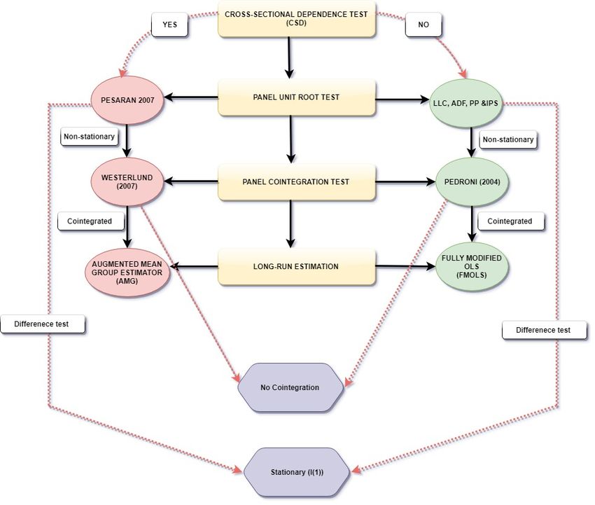
4. Theoretical Framework
After specifying the proposed models based on the respective hypotheses, we estimate
and investigate the direct, indirect, and mediating relationships amid variables used in the study. To be
able to select the right methods to provide robust results, we developed the analytical framework in
Sustainability
Figure 2. 2020, 12, x FOR PEER REVIEW 7 of 19
Figure 2. Analytical framework for estimating the affiliations amid analysed variables.
Figure 2. Analytical framework for estimating the affiliations amid analysed variables.
Step 1: Cross-Sectional Reliance Test
Step 1: Cross-Sectional Reliance Test
We conduct the cross-sectional reliance or dependence test to ascertain the spatial relationship
within Wethe
conduct
panel. the
Thecross-sectional relianceamid
spatial relationship or dependence test tounits
cross-sectional ascertain
may the spatial
arise relationship
because of high
within the
economic panel. and
linkages Theother
spatial relationship
common amid cross-sectional
factors among countries withinunits may arise
the panel. because
However, of high
the strength
economic linkages and other common factors among countries within the
of these economic linkages and other common factors has varied impacts across different units. panel. However, the
strength of these
Accordingly, economic
random linkages and sampled
and independently other common factors has varied
cross-sectional-units impactsmay
or countries across
notdifferent
resolve
units.complex
these Accordingly, random
forms of spatial and independently
and temporal sampled
dependence thatcross-sectional-units or countries
may exist within the panel may not
data. Therefore,
resolve
the these complex
interdependence mayforms of in
result spatial
someandformtemporal dependence
of cross-sectional that mayerrors
correlation exist in
within the panel
the panel data
data. Therefore,
applications andthe
caninterdependence may resultinferences.
lead to invalid statistical in some form of cross-sectional
Consequently, we findcorrelation
it prudent errors in
to test
for cross-sectional dependence to help determines the method to be used to carry out unit rootit
the panel data applications and can lead to invalid statistical inferences. Consequently, we find
prudent
and to test fortests.
cointegration cross-sectional dependence to help determines the method to be used to carry out
unit root and cointegration tests.
Step 2: Panel Unit Root Test
StepNext,
2: Panel
weUnit
test Root Test
the integration properties of the variables adopted for the study. The presence
or absence of cross-sectional reliance withinofthe
Next, we test the integration properties thepanel dataadopted
variables determines as to
for the whether
study. to employ
The presence or
first-generation
absence of cross-sectional reliance within the panel data determines as to whether to employtest
or second-generation unit root test. This is because first-generation unit root is
first-
efficient
generationfor cross-sectional independencies,
or second-generation unit root whereas
test. This second-generation unit root test
is because first-generation works
unit rootwell
test inis
the presence of cross-sectional correlations. Hence, the unavailability of cross-sectional
efficient for cross-sectional independencies, whereas second-generation unit root test works well affiliation will
in
lead to the use
the presence of of Levin, Lin, and
cross-sectional Chu (LL&C)
correlations. t-test;
Hence, the Im, Pesaran, and
unavailability Shin (IPS) test;affiliation
of cross-sectional Augmented will
lead to the use of Levin, Lin, and Chu (LL&C) t-test; Im, Pesaran, and Shin (IPS) test; Augmented
Dickey-Fuller-Fisher (ADF-Fisher) test; and Phillip-Perron Fisher (PP-Fisher) test as the first-
generation unit root test, whereas any evidence of cross-sectional connectedness will lead the study
to employ cross-sectional IPS (CIPS) and cross-sectional ADF (CADF) as the second-generation panel
unit root test. As per our assumption, when series are not stationary at any order, the analysisSustainability 2020, 12, 895 8 of 20
Dickey-Fuller-Fisher (ADF-Fisher) test; and Phillip-Perron Fisher (PP-Fisher) test as the first-generation
unit root test, whereas any evidence of cross-sectional connectedness will lead the study to employ
cross-sectional IPS (CIPS) and cross-sectional ADF (CADF) as the second-generation panel unit root
test. As per our assumption, when series are not stationary at any order, the analysis terminates.
Step 3: Panel Cointegration Test
Again, we conduct a co-integration test to examine the existence of structural long-run relationship
amid the series for the study. Thus in the presence of cross-sectional dependences, the Pedroni test,
which classified first-generation panel cointegration test will be employed, whereas in the presence
of the aforementioned issue, the Westerlund [29] test of cointegration will be used to examine
the long-run equilibrium relationship between variables. If the cointegration tests, whether first or
second generation fails to reject the null hypothesis of no cointegration, then the series cannot be
analysed, if not the analysis will proceed with estimating the panel data model.
Step 4: Estimation of Long-Run Relationship
Finally, we estimate the long-run relationships by employing an estimator in order to examine
the effects of the various explanatory variables on the corresponding response variables. Thus in
the presence of cross-sectional correlations the study is likely to employ the Augmented Mean
Group (AMG) estimator whereas on the other side where no issues of cross-sectional affiliations are
apparent the study opt for the Fully Modified Ordinary Least Square (FMOLS) estimator. Summarily,
the afore listed steps together form the analytical framework specified in Figure 2. Thus, going by
the cross-sectional dependence test results, there is evidence of cross-sectional independences; hence,
the study uses the first-generation econometric approaches listed on the right side of Figure 2. Details of
these first-generation econometric approaches to be used in the study due cross-sectional independencies
are briefly described as follows.
4.1. Cross-Sectional Dependence Test
Since the sampled countries have different attributes, the issue of cross-sectional reliance in the panel
could not be overlooked. Thus, the presumption of cross-sectional freedom is completely wrong in
panel data analysis. According to Pesaran [30], cross-sectional reliance within panels leads to bias
estimations as well as inconsistent standard errors of the estimated parameters. Hence, as part of
the empirical analysis process, we found out whether cross-sectional reliance existed in the model or not.
The presence of cross-sectional dependence or independence help determine the methods to be employed
for the tests of stationarity and co-integration. To serve as a robustness check, the Breusch-Pagan
LM test and the Pesaran scaled LM test are undertaken to authenticate the results. The Pesaran [30],
cross-sectional reliance test is grounded on the traditional panel data model expressed as
yi,t = αi + βi,t xi,t + µi,t , (6)
where i = 1, 2, . . . N and t = 1, 2 . . . , T, βi,t is a K × 1 vector of parameters to be estimated, xi,t also
represents a K × 1 vector of input variables, αi on the other hand indicates the time-invariant individual
nuisance estimates, and µi,t denotes the error terms that are assumed to be individually and identically
distributed. The test of null hypothesis of no cross-sectional reliance verses the alternative hypothesis
of the existence of cross-sectional connectedness is respectively expressed as
Ho : ρij = ρ ji = cor(µit , µ jt ) = 0 f or j , i, (7a)
HA : ρij = ρ ji = cor(µit , µ jt ) , 0 f or some j , i, (7b)Sustainability 2020, 12, 895 9 of 20
where ρij or ρ ji is the correlation coefficient obtained from the error terms of the model and is given by
the following relation:
PT
t=1 µit µ jt
ρij = ρ ji = P 1/2 P 1/2
. (8)
( Tt=1 µit 2 ) ( Tt=1 µ jt 2 )
Thus, considering the pairwise correlation coefficients ρ̂ij among the cross-sectional residuals,
the CD test statistic as proposed by Pesaran is computed below as
s
N−1 N
2T X X
CDP = ρ̂ij → N (0, 1). (9)
N (N − 1)
i=1 j=i+1
We applied the Breusch and Pagan [31], LM tests by obtaining the sum of squared coefficients
of correlation among cross-sectional residuals by means of OLS method. The LMBP test statistic is
computed by the formula:
N−1
X X N
LMBP = T ρ̂2ij , (10)
i−1 j=i+1
where ρ̂ij refers to the sample estimate of cross-sectional correlation among residuals. N and T are
number of cross-sections and time dimension, respectively and i denotes each individual. Given the null
hypothesis of no cross-sectional correlations, fixed N and T→∞, the CDLM1 is approximated to Chi
Square distribution with N(N − 1)/2 degrees of freedom.
The Pesaran [30] cross-sectional dependency Lagrange Multiplier (CDLM ) test sums the squares
of the correlation coefficient between cross-sectional residuals. The technique is used when T > N
or N > T, where N is the cross-sectional dimension and T is the time dimension of the panel, and is
asymptotically standard and normally distributed. The test is calculated using the formula
s
N−1 N
1 X X
CDLM = ( Tρ̂ij ), (11)
N (N − 1)
i=1 j=i+1
where ρ̂ij is previously defined as sample estimate of cross-sectional correlation among residuals.
The null hypothesis of this test is similar to CDP and LMBP tests.
4.2. Panel Unit Root Test (PURT)
Further, we analyzed the integration properties of the variables via unit root tests. The choice of
a particular unit root test to be used rely on the outcome of the cross-sectional reliance test because
there are two types of generations for the test of data stability. The first generation unit root tests are
more applicable to cross-sectional individuality, while the second generation tests work perfectly for
cross-sectional dependencies. Thus, due to the occurrence of cross-sectional independence among
residual terms within all cross-sections, the study employed the first generation panel unit root tests.
In testing the presence of unit root among the analyzed variables, the following equation is used:
∆yit = ρi yit−1 + δi Xi,t + εi,t , (12)
where i = 1, 2, . . . N for each country in the panel t = 1, 2 . . . , T stands for the time period, Xi,t denotes
the vector of exogenous variables of the model which contains fixed effects or individual time trend,
ρi symbolizes autoregressive coefficients, and εi,t is the error terms of stationary sequence. Specifically,
yit is considered to be weak in stationary trend if ρi < 1, otherwise if ρi = 1, yit is said to be haveSustainability 2020, 12, 895 10 of 20
a unit root. Due to autocorrelation which may occur in Equation (7), Levin et al. [32] developed a higher
order differential time-delay terms similar to the ADF test in the form
ρi
X
∆yit = ρi yit−1 + δi Xi,t + θij ∆yit−1 + εi,t , (13)
j=1
where ρi represents number of lags in the regression and εi,t in this case becomes the white noise.
Further Im et al. [32] specified a t-bar statistic as the mean of the individual ADF statistic in the form
N
1 X
t= tρi , (14)
N
i=1
where tρi signifies the individual t-statistic to test the null hypothesis of no stationarity. Generally,
the t-bar statistic is distributed with respect to the null hypothesis, where critical values for given
values of N and T are provided by Im et al. [32]. The LLC unit root test assumes ρi = ρ, meaning all
cross-sectional units are non-stationary, whereas Fisher-ADF test together with Fisher PP test permit ρi
to vary across different cross-sections. The Fisher-PP test employs the Phillips-Perron individual unit
root test to each cross-section; the test is robust to serial correlation. The combined p-value from both
tests is of the form
XN
2
ρ = −2 Inρi → X2N , (15)
i=1
where ρi is the p-value from the individual unit root test for cross-section i, the test statistics ρ follows
2 distribution with 2N degree of freedom as Ti→∞ for all N. The null hypothesis of unit root for
a X2N
all N cross section is written as
H0 : α = 0, for all i (i = 1, . . . , N). (16)
The alternative hypothesis is that some cross-sections have unit roots and is written as
α , 0 f or some i
(
H1 : . (17)
α < 0 f or other i
In the case of stable variables, their attributes are examined through regression analysis. Otherwise,
the process of analysis is to be terminated. At the attainment of stability (specifically after the first
difference), a co-integration test is conducted in the case of a multivariate model.
4.3. Panel Co-Integration Test
With the variables integrated at the same order, we proceed to examine whether the variables
are co-integrated in the long-run or not. The Pedroni [33] test and the Kao [34] test are employed.
These tests are adopted because they take into consideration cross-sectional independence with
individual effects. The Pedroni’s test for co-integration has seven (7) tests all distributed asymptotically
as standard normal. The first tests comprising of the panel v-statistic, panel ρ-statistic, panel PP-statistic,
and panel ADF-statistic, adopt a within dimension approach, while the second tests, consisting of
the group ρ-statistic, group PP-statistic, and group ADF statistic, adopt a between dimension approach.
The Pedroni panel co-integration test is built on the regression model in Equation (18) as follows:
yit = αi + δi t + β1i x1i,t + β2i x2i,t + . . . + βmi xmi,t + εit , (18)
where αi and βij are the intercepts and slope coefficients which can vary across cross-sections, t = 1, . . . , T,
i = 1, . . . , N, m = 1, . . . , M, x and y are assumed to be integrated of the same order (I(1)). The nullSustainability 2020, 12, 895 11 of 20
hypothesis of no co-integration of the Pedroni panel co-integration test is determined with respect to
the error term (εit ) which is expressed as
εit = ρi εit−1 + µit . (19)
The alternative hypothesis on the other hand includes the homogeneous hypothesis (HA :
ρi = ρ < 1) for all individual series for the within dimension test and heterogeneous alterative
(HA : ρi < 1) also for all individual series for between dimension test. Having established the existence
of co-integration among the variables, we proceed to determine the model form or the estimator to
be used to estimate the established model. Based on the determined model form, the elasticities of
variables within the specified models are examined for various inferences to be made.
4.4. Panel Model Estimation
To establish the co-integration of variables, it is necessary to pin down the long-run estimates
of the coefficients with respect to the explanatory variable. There are many estimators that can
analyze the association between the variables, but we opted for the Fully Modified Ordinary Least
Squares (FMOLS) estimator because the FMOLS provides more robust estimates in the presence
of cross-sectional independences and overcomes spurious regressions characterized by the OLS.
The FMOLS estimator is adopted because it caters for any potential endogeneity in the regressors
as a result of the existence of long-run affiliations between the explained and the explanatory variables.
Another essential reason for the adoption of the FMOLS estimator produces asymptotically unbiased
estimates; it further produces nuisance parameter free standard normal distributions. Inferences are
made regarding common long-run associations that are asymptotically invariant to the considerable
degree of short-run heterogeneity prevalent in studies typically associated with panels of aggregate
data [35].
As suggested by Pedroni [35], our model from Equation (5a) to Equation (5c) is respectively based
on the following regression equations:
Ki
X
ln FOAi,t lnNATMi,t lnNBBi,t = αi + βi lnMPTit + γik ∆lnMPTit−k + µit , (20)
k=−Ki
PK
ln FOAi,t lnNATMi,t lnNBBi,t = αi + βi lnMPTit + k=i −K γik ∆lnMPTit−k +
PK i (21)
δi lnPOPit + k=i −K τik ∆lnPOPit−k + µit ,
i
Ki 3 Kj 3
X X X X
FSRit = αi + βi lnMPTit + γik ∆lnMPTit−k + θ0i lnZi,t + θ0i lnZi,t−k + µit , (22)
k=−Ki i=1 k=−Ki i=1
for i = 1, 2, . . . , N and t = 1, 2, . . . , T. where lnFOAit , lnNATMit , lnNBBit , lnFSRit , and lnPOPit
represents the natural logarithm of formal account ownership, number of ATMs, number of bank
branches, financial sector rating and population whilst Zit is a vector representing natural logarithm of
system of control variables with respect to Equation (22). FOAit , NATMit , NBBit , FSRit , POPit and Zit
are cointegrated with slopes βi , δi , θ0i which may or may not be homogenous across i.
Let ξit = (µit , ∆MPTit , ∆POPit , ∆Zit ) be a stationary vector including the estimated residuals.
" #
T T
Also let Ωit = limT→∞ E T−1 ( ξit ) ξit 0 be the long-run covariance for the vector process which is
P P
t=1 t=1
decomposed into Ωi = Ω0i + Γi + Γ0i where Ω0i is the cotemporaneous covariance and Γi is a weightedSustainability 2020, 12, 895 12 of 20
sum of autocovariances. Relying on the aforementioned relations, the panel FMOLS estimators for βi ,
δi , and θ0i are respectively given by the following relations:
N T −1 N T
X X 2 X X
β̂∗NT −β = ( L̂−2
22i (lnMPTit − lnMPTi ) ) L̂−1 −1
11i L̂22i ( (lnMPTit − lnMPTi )µit ∗ − Tγ̂i ), (23)
i=1 t=1 i=1 t=1
N T −1 N T
X X 2 X X
δ̂∗NT −δ = ( L̂−2
22i (lnPOPit − lnPOPi ) ) L̂−1 −1
11i L̂22i ( (lnPOPit − lnPOPi )µit ∗ − Tτ̂I ), (24)
i=1 t=1 i=1 t=1
N T −1 N T
∗ 2
X X X X
θ̂i NT −δ = ( L̂−2
22i (Zit − Zi ) ) L̂−1 −1
11i L̂22i ( (Zit − Zi )µit ∗ − Tθ̂i ), (25)
i=1 t=1 i=1 t=1
Ω̂21i
where µit ∗ = (µit − µi ) −
Ω̂22i
∆lnMPTit , (µit − µi ) − Ω̂
Ω̂
21i Ω̂
∆lnPOPit and (µit − µi ) − 21i ∆lnZit respectively,
Ω̂
22i 22i
Ω̂21i
and γ̂i = Γ̂21i + Ω021i − (Γ̂22i + Ω022i ).
Ω̂22i
4.5. Heteroskedasticity and Serial Correlation Tests
After the estimation of the long-run relationships between the variables, we examined the validity
of the established model by testing for the presence or absence of heteroskedasticity and serial correlation
in the model. As postulated by Gujarati and Porter [36], the presence of heteroskedasticity or serial
correlation implies that the OLS estimators are no longer the Best Linear Unbiased Estimators (BLUE),
as they become inefficient leading to imprecise predictions. We employ the Breusch and Pagan [37]
test for heteroskedasticity and the Wooldridge [38] test for serial correlation. The former tested the null
hypothesis of homoscedasticity or the absence of heteroskedasticity in the established model, as against
the alternative hypothesis of the presence of heteroskedasticity in the model. The latter tested the null
hypothesis for the absence of serial correlation in the established model as against the alternative
hypothesis for the existence of serial correlation in the model.
5. Results and Discussion
5.1. Summary of Descriptive Statistics and Multicolinearity Test
A brief summary of the descriptive statistics is presented in Table 2. With respect to our findings,
the most important series refers to the actual deviation from the mean value of the variables proposed
in the study. To be more specific, the value of the standard deviation for mobile payment transaction
(MPT) is 5.84 with a standard deviation of 0.21. Furthermore, the same statistics for population
(POP), formal account ownership (FAO), number of ATMs (NATM), number of bank branches (NBB)
and financial sector rating (FSR) are respectively obtained as 9.56(2.39), 6.34(1.59), 6.19(1.55), 5.12(1.28),
and 7.52(1.88) where those in parenthesis represent the corresponding standard deviations. Further,
Table 2 gives the value on Skewness, kurtosis, and JB tests, which helps to verify whether the series
with the employed data follows the normal distribution. It is inferred that the response variable
POP, FAO, NATM, and FSR are negatively skewed with the exception of MPT and NBB which are
flattened to the right (positively skewed) compared to the normal curve. Also the kurtosis values of
the variables which include POP, NATM, and NBB are found to have a mesokurtic shape in the because
they respectively have their kurtosis values to be approximately three, whereas FAO and FSR are
evidenced to be platykurtic in terms of shape since their values of kurtosis are approximately less
than three. None of the variables used in the study with respect to the conceptual model in Figure 1
are evidenced to be mesokurtic. Generally, the normal value of the Skewness is expected to be
approximately “0” and that of kurtosis to be approximately “3” when the observed series is normally
distributed. The result per the kurtosis and the Skewness for the various variables used in the study isSustainability 2020, 12, 895 13 of 20
in line with the Jarque-Bera tests statistics in which all respective values are not approximately zero
or exactly zero. The JB test is used to determine whether the given series is normally distributed
or not, with the null hypothesis that the series follows a normal distribution against the alternative
hypothesis that the series is otherwise. The result from the JB test therefore rejects the null hypothesis
that the series is normally distributed all at 1% level of significance.
Table 2. Summary of descriptive statistics.
Variable Mean Std. Dev. Skewness Kurtosis Jarque-Bera Test
Mobile payment transaction 5.84 0.21 0.75 1.64 19.83 a
Population 9.56 2.39 −0.49 2.46 55.32 a
Formal account ownership 6.34 1.59 −1.32 2.38 30.64 a
Number of ATMs 6.19 1.55 −1.63 2.53 45.20 a
Number of bank branches 5.12 1.28 1.25 2.64 26.58 a
Financial sector rating 7.52 1.88 −1.83 2.20 58.98 a
Note: a means significance at 1%.
To help identify the existence of highly correlated variables which might not be worthy of inclusion
in a specific model as an explanatory variable, we tested for multicolinearity among the explanatory
variables in the various panel regression models specified using the Variance Inflation Factor (VIF)
and Tolerance. In conducting the test, only Model 1 is excluded since it has one explanatory variable
hence no need to investigate the existence of multicolinearity. Multicolinearity is examined in regression
models with multiple regressors such as our Models 2 and 3. Table 3 shows the multicolinearity test
results with respect to the independent variables used in the study. The VIF values are significantly
less than 10 whilst the values of the tolerance on the other hand are also more than 0.2. It implies that
there exist no multicolinearity among the variables in both multiple linear regression models in Models
2 and 3. Since there exist no multicolinearity in the multiple linear regressions specified in the study,
this implies that all the variables used in the study are maintained in their respective models.
Table 3. Test of multicolinearity.
Model Independent Variables VIF Tolerance
MPT 8.250 0.472
Model 2
POP 5.216 0.761
MPT 1.773 0.833
FAO 1.892 0.885
Model 3
NATM 4.281 0.820
NBB 9.175 0.757
Note: The values of both the variance inflation factor (VIF) and Tolerance are based on the response variables in
Models 2 and 3. The VIF values are below 10 and those of Tolerance below 0.2. MPT, POP, FAO, NATM, and NBB
represents mobile payment transaction, population, formal account ownership, number of ATMs, and number of
bank branches respectively.
5.1.1. Cross-Sectional Residual Dependence Test
Prior to the empirical analysis, cross-sectional reliance tests as mentioned in the earlier section is
be performed on the panel data employed. The results based on three different tests of cross-sectional
dependence which includes the Breusch and Pagan LM test, Pesaran scaled LM, and Pesaran CD
tests are reported in Table 4. As shown in the table, outcomes from the aforementioned CD tests
employed all failed in rejecting the null hypothesis of cross-sectional independence at 10% level of
significance. The cross-sectional residual reliance across country groups therefore cannot be considered.
With the failure to reject the null hypothesis of cross-sectional independence, the study adopts first
generation panel unit root tests which include Levin, Lin and Chu (LL&C) t-test, Im, Pesaran and Shin
(IPS) test, Augmented Dickey-Fuller Fisher (ADF-Fisher), and Phillips-Perron Fisher (PP-Fisher)
to examine the integration properties of employed variables.Sustainability 2020, 12, 895 14 of 20
Table 4. Test results from the cross-sectional dependence test.
Panel CD-Test Statistic CD-Test Value Probability Value
Breusch and Pagan LM test 21.399 0.559
Africa Pesaran scaled LM −0.427 0.636
Pesaran CD −0.318 0.830
Note: The null hypothesis of cross-sectional independence is rejected at 10% level of significance.
5.1.2. Panel Unit Root Test
Prior to conducting the panel cointegration test to examine the existence of long-run affiliations
amid variables employed for the study, we investigate the integration properties of these variables.
The panel unit root tests commonly used as reported in Table 5 are the Levin, Lin, and Chu (LL&C) t-test;
the Im, Pesaran, and Shin (IPS) test; Augmented Dickey-Fuller Fisher (ADF-Fisher); and Phillips-Perron
Fisher (PP-Fisher). The test results reveal the variables to be analysed are not stationary at their level
forms but rather become stationary when differenced in the first order. Thus the variables employed
within the study are integrated at the same order (I(1)).
Table 5. Panel unit root test results.
Form Variable LL&C IPS ADF-Fisher PP-Fisher Decision
Level MPT 3.397 0.343 5.855 2.356 Not stationary
POP 3.780 0.302 10.780 3.932 Not stationary
FAO 1.522 4.367 0.695 0.543 Not stationary
NATM 5.577 8.708 0.070 0.084 Not stationary
NBB −0.422 1.092 4.408 11.423 Not stationary
FSR 5.167 1.799 7.581 6.198 Not stationary
First Difference MPT −5.205 a −4.723 a 34.767 a 45.612 a Stationary
POP −2.652 a −2.224 b 22.078 b 27.608 a Stationary
FAO −4.412 a −4.380 a 41.043 a 35.086 a Stationary
NATM −2.854 a −2.146 b 24.368 b 29.846 a Stationary
NBB −5.330 a −1.681 b 23.587 b 29.816 a Stationary
FSR −2.273 b −1.629 b 23.104 b 57.915 a Stationary
Note: a and b mean significance at 1% and 5% levels.
5.1.3. Panel Cointegration Test
Relying on the results of the panel unit root tests in the previous section, eleven different
cointegration statistics from the Pedroni cointegration test are calculated to test the long-run relationship
between variables employed in the three models proposed for the study. Results pertaining to the panel
cointegration test developed by Pedroni [33] are reported in Table 6. The results obtained from Model
1 for the subpanels made up of FOA, NATM, and NBB with MPT as the only explanatory variable
indicating nine (9) test statistics are significant, thus implying MPT serves as the only independent
variable in Model 1 with a co-integrating affiliation with FAO, NATM, and NBB respectively. In the same
manner, no less than nine statistics from Models 2 and 3 are identified to be statistically significant,
thereby rejecting the null hypothesis of no co-integration. The results indicate, POP together with
MPT in Model 2 are cointegrated with FAO, NATM, and NBB correspondingly whereas in Model 3 all
the explanatory variables which includes FAO, NATM, NBB, and MPT have a long-run relationship
with FSR. In summary, the Pedroni panel cointegration test results suggest that the variables are
cointegrated in the three models proposed for the study.Sustainability 2020, 12, 895 15 of 20
Table 6. Results from panel cointegration test.
Model 1 Model 2 Model 3
FOAi,t NATMi,t NBBi,t FOAi,t NATMi,t NBBi,t FSRi,t
Alternative Hypothesis: Common AR Coefficients (within Dimension)
Panel v-statistic −3.927 −1.515 −3.308 0.330 1.709 −0.938 −3.504
Panel a a a a a a
−33.684 −29.789 −18.554 −17.785 −16.809 −14.508 −13.263 a
rho-statistic
Panel
−181.553 a −209.863 a −125.819 a −85.611 a −100.129 a −70.941 a −75.525 a
PP-statistic
Panel
−79.535 a −58.669 a −43.661 a −30.905 a −31.246 a −35.815 a −28.507 a
ADF-statistic
Weight Statistics
Panel v-statistic −6.710 −7.766 −2.708 −2.980 −3.703 −2.549 −4.407
Panel
−24.352 a −24.512 a −17.683 a −17.614 a −19.765 a −17.468 a −14.033 a
rho-statistic
Panel
−168.746 a −177.961 a −83.418 a −84.007 a −101.225 a −77.050 a −90.550 a
PP-statistic
Panel
−60.700 a −60.176 a −42.915 a −37.993 a −25.385 a −35.066 a −27.257 a
ADF-statistic
Alternative Hypothesis: Individual AR Coefficients (between Dimension)
Group
−22.087 a −22.625 a −15.419 a −18.546 a −16.405 a −16.938 a −11.816 a
rho-statistic
Group
−139.279 a −156.963 a −122.402 a −102.209 a −133.050 a −106.065 a −130.006 a
PP-statistic
Group
−79.719 a −78.917 a −50.771 a −35.615 a −35.211 a −45.203 a −43.996 a
ADF-statistic
Note: a means significance at 1% level.
5.2. Estimation of Panel Models
Results from our Model 1 depicted in Table 7 which assesses the direct relationship between
mobile payment transactions and formal account ownership, the number of ATMs, and the number of
bank branches, show positive significant relationship between our predictors and explanatory variable
respectively. Indicatively, the recent rise in the overall financial inclusion figures in the region is partly
driven by the competition offered by mobile payment operators [2]. This partly debunks on-going
debates about the negative effects of mobile payment on traditional financial institutions survival [3,39].
Rather, this provides deeper insight into the positive aspects technology development towards
the financial landscape in the region [3,40,41]. While recent studies [3,15,39,42] point to the singular role
of mobile payment in financial inclusion in the region, the result with coefficient of 0.582 and an R-square
of 0.338 indicates that the increase in mobile payment transactions also significantly affect traditional
banks number of formal account ownership numbers in the region. Practically, to stimulate growth
in the financial sector of a region characterized mostly by rural settlements which limits rapid
investments in physical financial infrastructure could benefit from the on-going competition [43].
Further, the increase in mobile payment transactions in the region significantly impacts on the growth
in the number of bank branches per 100,000 adults judging from the results with a coefficient of 0.552
and an R-square of 0.305. Finally, the increase in mobile payment causes traditional banks to set up more
bank branches as the result indicates a positive relationship with the coefficient of 0.533 and an R-square
of 0.285. This explanatory variable is a key indicator of financial accessibility in traditional financial
institutions as indicated by Ahamed and Mallick [28], and supports the strong institutional structure
of traditional financial institution which makes disruptive technologies difficult to completely change
their usual offerings [12,25]. To expound, Banks in the region continue to invest in new ATM machines
and invest in new bank branches in areas previously classified as undesired without replacing their
old services because of the need to survive as a result of the competition from the mobile payment
operators [24]. Our second model result depicted in Table 7 which measures the mediating role ofYou can also read