The Berkeley Environmental Air-quality and CO2 Network: field calibrations of sensor temperature dependence and assessment of network scale CO2 ...
←
→
Page content transcription
If your browser does not render page correctly, please read the page content below
Atmos. Meas. Tech., 14, 5487–5500, 2021
https://doi.org/10.5194/amt-14-5487-2021
© Author(s) 2021. This work is distributed under
the Creative Commons Attribution 4.0 License.

The Berkeley Environmental Air-quality and CO2 Network: field
calibrations of sensor temperature dependence and assessment of
network scale CO2 accuracy
Erin R. Delaria1 , Jinsol Kim2 , Helen L. Fitzmaurice2 , Catherine Newman1 , Paul J. Wooldridge1 , Kevin Worthington1 ,
and Ronald C. Cohen1,2
1 Department   of Chemistry, University of California Berkeley, Berkeley, CA 94720, USA
2 Department   of Earth and Planetary Science, University of California Berkeley, Berkeley, CA 94720, USA

Correspondence: Ronald C. Cohen (rccohen@berkeley.edu)

Received: 29 April 2021 – Discussion started: 11 May 2021
Revised: 13 July 2021 – Accepted: 18 July 2021 – Published: 12 August 2021

Abstract. The majority of global anthropogenic CO2 emis-          regions are needed to assess progress toward emissions com-
sions originate in cities. We have proposed that dense net-       mitments.
works are a strategy for tracking changes to the processes           Monitoring trends in CO2 emissions by tracking ambi-
contributing to urban CO2 emissions and suggested that a          ent CO2 in urban environments is challenging because of
network with ∼ 2 km measurement spacing and ∼ 1 ppm               the large diversity of emissions sources, complex spatial and
node-to-node precision would be effective at constraining         temporal patterns of emission rates, varied topography, and
point, line, and area sources within cities. Here, we report on   the effects of meteorology on the observed concentrations
an assessment of the accuracy of the Berkeley Environmen-         (e.g., Vardoulakis et al., 2003; Lateb et al., 2016). As a result,
tal Air-quality and CO2 Network (BEACO2 N) CO2 mea-               most cities rely exclusively on economics and social data and
surements over several years of deployment. We describe a         do not check whether their reported emissions match the ob-
new procedure for improving network accuracy that accounts        served CO2 enhancements in the air over their city. To date,
for and corrects the temperature-dependent zero offset of the     most efforts to assess CO2 emissions from cities have re-
Vaisala CarboCap GMP343 CO2 sensors used. With this cor-          lied upon a small number of high-cost CO2 instruments that
rection we show that a total error of 1.6 ppm or less can be      provide precise and accurate representations of regional sig-
achieved for networks that have a calibrated reference loca-      nals. Other approaches include use of correlations between
tion and 3.6 ppm for networks without a calibrated reference.     CO2 and other gases, measurements of 14 C in annual grasses,
                                                                  and use of satellite column CO2 observations such as from
                                                                  OCO-2 (e.g., Pataki et al., 2003, 2006; Riley et al., 2008;
                                                                  Thompson et al., 2009; Kort et al., 2013; Andrews et al.,
1   Introduction                                                  2014; Fu et al., 2019; Ye et al., 2020). Most of these ef-
                                                                  forts have used as a target metric an annual average of fossil
The atmosphere has warmed approximately 1 ± 0.2 ◦ C since         fuel-related CO2 emissions from an entire city (e.g., McK-
pre-industrial times, which is unequivocally due to an-           ain et al., 2012; Kort et al., 2013; Bréon et al., 2015; Ver-
thropogenic emissions of CO2 and other greenhouse gases           hulst et al., 2017). Simultaneous measurements of CO and
(GHGs) (IPCC, 2021). Global initiatives are needed to limit       14 CO have also provided information about sector-specific
                                                                         2
warming to 1.5 ◦ C by achieving net zero GHG emissions            emission sources (Turnbull et al., 2015). Other methods of
by 2050 and a 45 % emissions decline from 2010 levels by          evaluating urban emissions have relied on emissions inven-
2030 (Rogelj et al., 2021). As over 70 % of global anthro-        tories (e.g., Gurney et al., 2009; Gately et al., 2013, 2017).
pogenic CO2 emissions originate from cities (United Na-           These emissions inventories are frequently applied to inverse
tions, 2011), effective CO2 monitoring strategies in urban

Published by Copernicus Publications on behalf of the European Geosciences Union.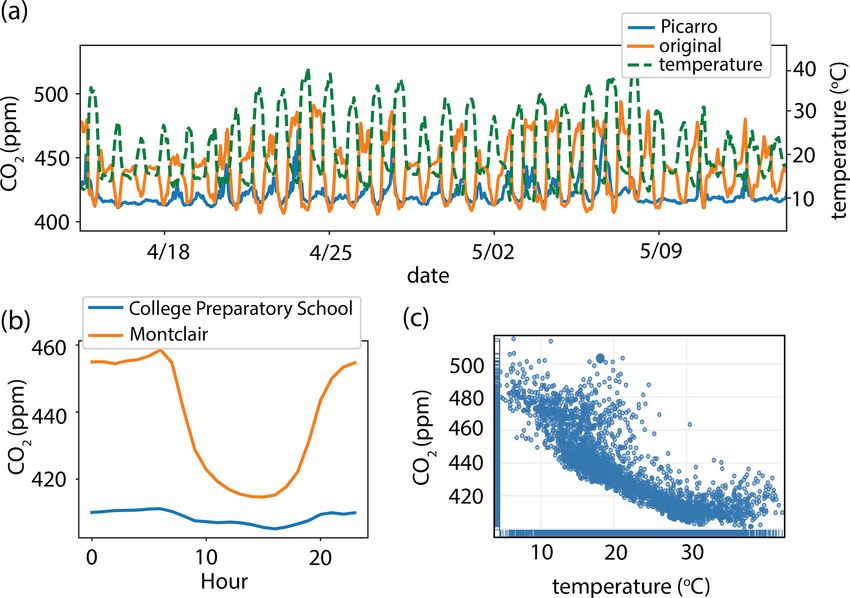
5488               E. R. Delaria et al.: BEACO2 N CO2 measurement accuracy and temperature dependence calibration

modeling approaches in combination with either short-term
mobile measurements or a small number of long-term mea-
surement sites to extract regional emissions (e.g., Brondfield
et al., 2012; Sargent et al., 2018; Nathan et al., 2018; Turnbull
et al., 2019). Several studies have also combined a network of
CO2 observations with inverse modeling approaches to eval-
uate the accuracy of emissions inventories and CO2 sources
(e.g., Lauvaux et al., 2016, 2020).
   We are pursuing a distinct approach aimed at process-level
understanding of the components of an urban emissions in-
ventory. To do so, we are developing tools for the deployment
of spatially dense networks of CO2 measurements, in com-
bination with gases and aerosols that are co-emitted and that
affect air quality. The result is an ability to map emissions
with ∼ 1 km or “neighborhood scale” fidelity. The Berkeley
Environmental Air-quality and CO2 Network (BEACO2 N)
(Turner et al., 2020; Kim et al., 2018; Shusterman et al.,
2018, 2016; Turner et al., 2016) is our platform for research
and development of tools for dense networks. New deploy-
ments in Glasgow, Scotland and Los Angeles, California are
bringing new collaborators and experience in different cities
to the project. BEACO2 N has been operating since 2012 in
the San Francisco Bay area and consists of over 70 nodes sep-
arated by approximately 2 km (Fig. 1). The nodes incorporate
commercially available, low-cost sensors for measuring CO,
NO, NO2 , O3 , particulates, and CO2 .
   Turner et al. (2016) assessed the performance of a hypo-
thetical BEACO2 N-like observing system coupled to an in-
verse model and demonstrated that a random measurement
uncertainty of 1 ppm between nodes was adequate to mean-            Figure 1. Map of all Bay Area BEACO2 N sites (small red dots),
ingfully constrain CO2 emissions from a point, line, or area        BEACO2 N sites discussed in this work (large blue dots), and the
                                                                    Richmond Field Station (star).
source of 147, 45, and 9 t C h−1 , respectively. With a 1 ppm
mismatch error, weekly CO2 emissions in the San Francisco
Bay area could be estimated to within 5 % error. In this paper
we describe advances in our approach to maintaining stable,         sensors (with off-the-shelf reported errors of 5–20 ppm) for
multiyear comparability among BEACO2 N nodes in a city              environmental variables, the median root mean square error
and evaluate the accuracy achieved with these new proce-            could be reduced to below 2 ppm, making the sensors po-
dures. Our emphasis in the revised approach to sensor ac-           tentially useful for ambient air-quality monitoring. Recently,
curacy is on tracking and correcting the temperature depen-         Müller et al. (2020) evaluated the potential applications of
dence of the Vaisala CarboCap GMP343 CO2 instruments.               a low-cost CO2 NDIR sensor network for resolving site-
We present the development and evaluation of the meth-              specific CO2 signals in Switzerland. The calibration method
ods using observations from the San Francisco Bay Area              of Müller et al. (2020) involved laboratory chamber calibra-
BEACO2 N deployment and then apply these ideas to the               tions of over 300 low-cost NDIR CO2 sensors and ambient
BEACO2 N network in Houston, Texas.                                 colocation with a reference instrument prior to deployment,
                                                                    as well as regular monitoring and drift correction during a 2-
                                                                    year deployment period. Shusterman et al. (2016) developed
2   Development of a CO2 field calibration method for               an in situ method for calibrating and correcting for individual
    Vaisala temperature dependence                                  instrument biases and temporal drifts of the Vaisala Carbo-
                                                                    Cap GMP343 CO2 instruments deployed in the BEACO2 N
The efficacy of a network of a large number of low-cost             nodes. Using this method, Shusterman et al. (2018) demon-
nondispersive infrared (NDIR) CO2 sensors to evaluate CO2           strated that the BEACO2 N network could provide highly sen-
emissions has been previously discussed (Shusterman et al.,         sitive detection of changes to traffic emissions at a scale rel-
2016; Turner et al., 2016; Martin et al., 2017; Shusterman          evant to policy concerns. Shusterman et al. (2018) also il-
et al., 2018; Müller et al., 2020). Martin et al. (2017) showed     lustrated the efficacy of the BEACO2 N network in show-
that after correcting six SenseAir K30 carbon dioxide NDIR          ing both regional CO2 emissions and local CO2 enhance-

Atmos. Meas. Tech., 14, 5487–5500, 2021                                              https://doi.org/10.5194/amt-14-5487-2021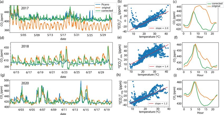
E. R. Delaria et al.: BEACO2 N CO2 measurement accuracy and temperature dependence calibration                                      5489

ments at the scale of a single neighborhood. In an analysis        ric particulate matter sensor and several Alphasense elec-
of the BEACO2 N observations for 6 weeks before and after          trochemical sensors for measuring CO, NO, NO2 , and O3
the COVID-19 shutdown, Turner et al. (2020) showed that            (CO-B4, NO-B4, either NO2-B42F or NO2-B43F, and ei-
a 25 % change in emissions is easily derived by an inverse         ther Ox-B421 or Ox-B431). The most recent version adds
model and that hourly variations in emissions can be inferred.     a Plantower PMS 5003 aerosol sensor. Sensors are assem-
   The use of a large number of low-cost CO2 sensors intro-        bled into compact, weatherproof enclosures with air flow
duces challenges regarding accuracy and inconsistent behav-        through the enclosure provided by two 30 mm fans. Data
ior between instruments that often requires labor-intensive        are compiled with a Raspberry Pi microprocessor and an
regular calibration, data correction and filtering, and vali-      Adafruit Metro Mini microcontroller. Data are acquired ev-
dation with comparison to a smaller number of frequently           ery 5 or 10 s and are transferred to a central server via an
calibrated high-accuracy instruments. In particular, the low-      Ethernet or Wi-Fi connection. Observations are posted on the
cost NDIR absorption sensor used in each BEACO2 N node             BEACO2 N website within a few hours of measurement time
(Vaisala CarboCap GMP343) is susceptible to temporal drift         (http://beacon.berkeley.edu, last access: 14 June 2021).
and fluctuations due to environmental variables that present          The Vaisala CarboCap GMP343 instrument uses pulsed
challenges to achieving a goal of 1 ppm network error (van         light from a filament lamp, which is reflected and refocused
Leeuwen, 2010; Shusterman et al., 2016). Correction of the         on an IR detector located behind a Fabry-Perot Interferom-
Vaisala CarboCap GMP343 instruments (Vaisala, hereafter)           eter (FPI). The FPI is electrically tuned so that its passband
for changes in pressure, temperature, and humidity is re-          corresponds to either the absorption wavelength of CO2 or
quired for accurate measurements (Vaisala, 2013). The typ-         a reference band (Vaisala, 2013). The calibration procedure
ical correction for pressure and temperature accounts for          for the Vaisala CarboCap GMP343 CO2 sensor is as out-
changes in the number density of CO2 according to the ideal        lined in Shusterman et al. (2016, 2018). Briefly, deployed
gas law (van Leeuwen, 2010; Vaisala, 2013; Shusterman              Vaisala sensors operate with the internal relative humidity
et al., 2016). The humidity effect on measured CO2 is ac-          (RH), temperature, and pressure compensation set to “off”
counted for by considering the dilution effect of water vapor      and the oxygen correction set to “on”, with oxygen input
according to Dalton’s law of partial pressures (van Leeuwen,       as 20.95 %. A post hoc multiplicative scale factor is ap-
2010; Vaisala, 2013; Shusterman et al., 2016). However,            plied to convert the raw CO2 outputs to the mole fraction
even after accounting for these factors, reported corrected        of CO2 that would be measured if the observed air parcel
CO2 concentrations for the Vaisala instrument have been ob-        were dried and brought to standard temperature and pres-
served to exhibit a strong temperature dependence of up to         sure (STP) ([CO2 ]STP ). Raw CO2 data are adjusted using
1 ppm ◦ C−1 (van Leeuwen, 2010). Using a laboratory cali-          temperature (T ) measured by the internal thermometer of
bration procedure, van Leeuwen (2010) found that a linear          the Vaisala. Water vapor pressure (PH2 O ) and air pressure
correction was necessary to account for the residual temper-       (Ptot ) are obtained from the pressure and dew point temper-
ature dependence. However, correcting for the temperature          ature measured inside each node enclosure by a Bosch Sen-
dependence using lab calibrations is labor intensive, as the       sortec Adafruit BME280 sensor. The [CO2 ]STP is then ad-
temperature dependence is unique for each Vaisala sensor.          justed to account for temporal drift in the instrument “zero”
Regular laboratory temperature calibration would also be re-       by comparing the background signal of the Vaisala CO2 mea-
quired to account for temporal variations in the temperature       surement at each node to a reference Picarro G2301 sys-
correction as sensors age. For a high-density urban network        tem, located at the Richmond Field Station in Richmond, CA
like BEACO2 N, this would require substantial time invest-         (Fig. 1). A moving 3-week window of the 10th percentile of
ment by trained personnel. The associated high labor costs         Vaisala CarboCap CO2 data Vaisala [CO2 ]10 % is generated
defeat the purpose of using low-cost sensors. In situ field cal-   and compared with the 10th percentile          of the reference Pi-
                                                                   carro instrument Picarro [CO2 ]10 % . The difference between

ibration of the Vaisala sensors thus presents a more attractive
method for correcting for the temperature dependence of the        Vaisala [CO ]           Picarro [CO ]
                                                                                2 10 % and            2 10 % is used to define the off-
CO2 measurements.                                                  set of the Vaisala instrument      [CO   ]drift . A linear correla-
                                                                                                           2 offset
                                                                   tion between [CO2 ]drift

                                                                                            offset and time is generated and used
                                                                   to calculate the drift-corrected CO2 data, [CO2 ]drift

2.1   BEACO2 N network                                                                                                         corrected
                                                                   (Eqs. 1–2):
The Berkeley Environmental Air-quality and CO2 Network
(BEACO2 N) Bay Area deployment currently consists of 73              [CO2 ]drift
                                                                             offset = mt × days + b                                   (1)
nodes spaced at ∼ 2 km intervals with locations in Alameda,
San Francisco, Contra Costa, Sonoma, Sacramento, and               [CO2 ]drift
                                                                         corrected = [CO2 ]STP − mt × days − b,                       (2)
Solano counties. A full description of a BEACO2 N node
                                                                   where mt is the temporal drift (ppm d−1 ) and b is a constant
can be found in Kim et al. (2018). Briefly, each node con-
                                                                   atemporal bias.
tains a nondispersive infrared Vaisala CarboCap GMP343
CO2 sensor, along with a Shinyei PPD42NS nephelomet-

https://doi.org/10.5194/amt-14-5487-2021                                               Atmos. Meas. Tech., 14, 5487–5500, 2021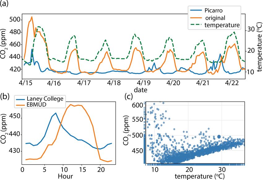
5490 E. R. Delaria et al.: BEACO2 N CO2 measurement accuracy and temperature dependence calibration
2.2 Picarro reference instrument
A “supersite” with reference grade instruments is oper-
ated within the BEACO2 N Bay Area network to provide
a reference for the network calibration. Instruments are in-
stalled within a temperature-controlled instrument shelter
at the U.C. Berkeley Richmond Field Station. Measure-
ments include basic meteorology, NOx (Thermo 42CTL with
a molybdenum NO2 to NO converter), O3 (Teledyne/API
T400), CO2 , CH4 , and CO (Picarro G2401 cavity ring down
analyzer). Air is sampled through Teflon tubes mounted to a
small tower affixed to the trailer roof, for a combined height
of 6 meters above the ground. The colocated BEACO2 N
node is attached outside of the trailer to the same tower.
The NOx and Picarro analyzer calibrations are checked
against reference gases every 2 to 3 weeks. The reference Figure 2. (a) CO2 mixing ratios from April 2020 at EBMUD and
gas cylinders for NOx , CO, and CH4 are Certified Standard measured with a Picarro instrument at the Richmond Field Station
grade from Praxair, and for CO2 are from the NOAA Global supersite. (b) EBMUD 2020 diurnal cycle compared with Laney
College. (c) Temperature dependence of the CO2 signal at EBMUD.
Monitoring Laboratory (two levels: 403.61 and 687.47 ppm).
The Picarro checks are made by flowing the sequence of ref-
erences gases into a tee at the inlet of the instrument for is a diurnal cycle that peaks midday (Fig. 2b). Figure 2b
15 min per step. The sequence of steps is performed twice compares the CO2 diurnal cycle at EBMUD with the nearby
during a check. The flow rate is set to be larger than the urban site Laney College (Fig. 1). In contrast to EBMUD,
instrument sample flow (0.4 L min−1 ) to overflow the inlet. Laney College exhibits a daily maximum at mid-morning–
The O3 analyzer is checked against a photometric calibrator a pattern more consistent with typical urban CO2 behavior
(Teledyne/API 703E). (Idso et al., 2002; Coutts et al., 2007; Turnbull et al., 2015;
Shusterman et al., 2016).
2.3 Identification of a temperature-dependent error in The Vaisala temperature dependence varies in magnitude
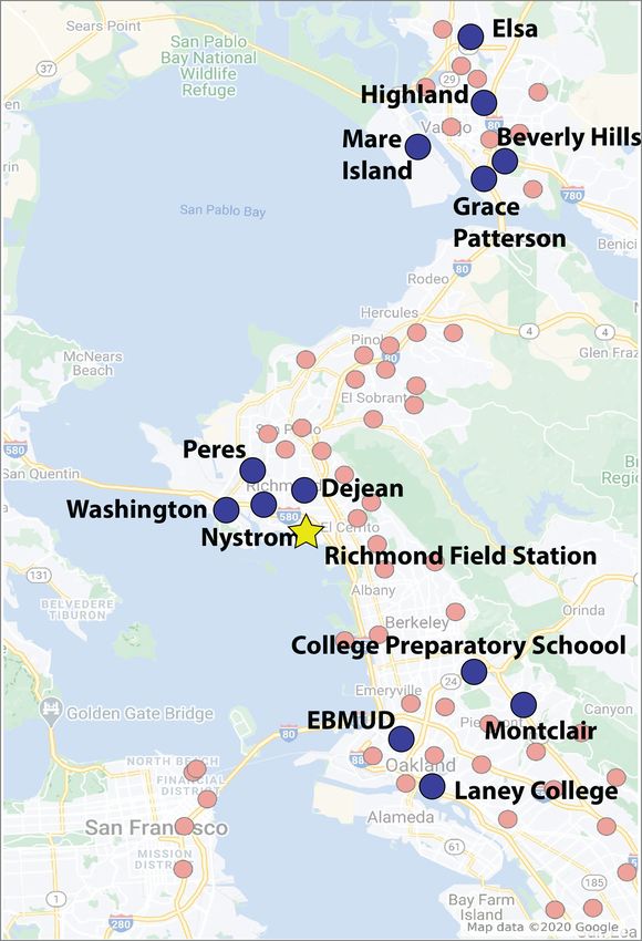
Vaisala measurements and sign. Figure 3 shows the CO2 mixing ratios and temper-
ature dependence at the Montclair Elementary School site.
There exists an additional temperature dependence among Compared to the Picarro instrument, this site also demon-
the Vaisala CarboCap GMP343 instruments that varies be- strates higher amplitude diurnal cycles (Fig. 3a), but these
tween instruments. The temperature dependence was first diurnal cycles are in phase with the reference instrument.
identified from observations of CO2 diurnal cycles at cer- Unlike EBMUD, the Montclair site exhibits a negative tem-
tain Bay Area BEACO2 N sites that were out of phase or perature dependence (Fig. 3c). Figure 3b shows the diurnal
larger in magnitude than the diurnal cycles at nearby nodes cycles at Montclair and the nearby node located at College
or measured by the Picarro. The presence of a temperature Preparatory School (CPS). The comparison of these two sites
dependence in suspect Vaisala instruments was confirmed by suggests there may indeed be an amplification of the diurnal
examining the relationship between temperature in the node cycle at Montclair caused by a negative temperature depen-
and the difference between baseline CO2 signals measured dence of the Vaisala instrument.
by the Vaisala and the Picarro reference instrument.
Diurnal cycles of urban CO2 typically exhibit a daily max- 2.4 Temperature correction method
imum at night or mid-morning (depending on influence from
traffic emissions) due to mixing in a shallow nighttime plan- The goal of our approach to accounting for the temperature
etary boundary layer (PBL), and reach a minimum during dependence of the Vaisala instruments is to rely exclusively
the day as PBL height increases and vegetation takes up CO2 on the network itself and, if available, supplementary refer-
(Idso et al., 2002; Coutts et al., 2007; Turnbull et al., 2015; ence instruments, such as a Picarro, for derivation of correc-
Shusterman et al., 2016). The presence of an additional tem- tion factors to null sensor temperature dependence.
perature dependence in the Vaisala CO2 instrument is partic- The method we developed builds on our method for ac-
ularly pronounced and obvious in the measurements obtained counting for drift in the instrument zero. To derive a tem-
with the sensor located at the East Bay Municipal Utility Dis- perature factor, we use hourly averaged [CO2 ]STP and node
trict (EBMUD) BEACO2 N site during 2020 (Fig. 2). The measurements of temperature (T ). It is important to note that
magnitude of the diurnal cycle at EBMUD is larger and out a major factor contributing to the temperature inside the node
of phase with the Picarro reference instrument (Fig. 2a). The is whether the node is placed in the sun or shade. As a re-
result of this temperature dependence at EBMUD (Fig. 2c) sult, direct correlation with meteorological temperature mea-
Atmos. Meas. Tech., 14, 5487–5500, 2021 https://doi.org/10.5194/amt-14-5487-2021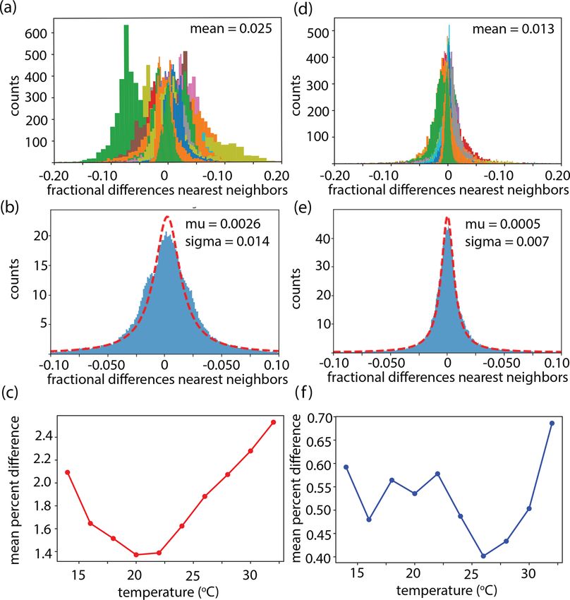
E. R. Delaria et al.: BEACO2 N CO2 measurement accuracy and temperature dependence calibration                                                  5491

                                                                    checks for agreement between neighboring sensors. Shifts in
                                                                    the offset bias, the temperature-dependent slope, or the time-
                                                                    dependent drift appear as sudden or gradual offsets in mix-
                                                                    ing ratios measured by a sensor and its neighbors. Typical
                                                                    identified shifts in the offset bias, the temperature-dependent
                                                                    slope, or the time-dependent drift are on the order of 10 ppm,
                                                                    0.5 ppm ◦ C−1 , and 0.1 ppm d−1 , respectively:

                                                                    [CO2 ]Toffset =1 [CO2 ]T10 % −med mT × T                                     (4)
                                                                                                         med
                                                                    [CO2 ]Tcorrected   = [CO2 ]STP −           mT × T .                          (5)

                                                                       An example calibration, demonstrating mT and [CO2 ]Toffset
                                                                    over time at EBMUD 2020, is shown in Fig. S1 in the Sup-
                                                                    plement. Following calculation of the temperature-corrected
                                                                    offset, the temporal drift slope and intercept of this corrected
Figure 3. (a) CO2 mixing ratios from May 2018 at Montclair and      offset are calculated and corrected using the methods de-
measured with a Picarro instrument at the Richmond Field Station    scribed above, resulting in the generation
                                                                                                                of the temperature-
supersite. (b) Montclair 2018 diurnal cycle compared with College                                            T ,drift
                                                                    and drift-corrected CO2 offset [CO2 ]offset .
Preparatory School. (c) Temperature dependence of CO2 signal at
Montclair.                                                           The final  temperature- and drift-corrected CO2
                                                                     [CO2 ]Tcorrected
                                                                              ,drift
                                                                                      is then calculated as

sured outside the node is not strong. For a moving three-
week window, at each hour (h), the lowest 10th percentile           [CO2 ]Tcorrected
                                                                            ,drift
                                                                                     = [CO2 ]STP −med mT × T − [CO2 ]Toffset
                                                                                                                        ,drift
                                                                                                                               .                 (6)
of [CO2 ]STP within ±1 ◦ C of T (h) is calculated. A running
array of temperature-based 10th percentile data is created for
                                                                       The majority of the BEACO2 N nodes examined demon-
both the Picarro supersite Picarro [CO2 ]T10 % at the Richmond
                                                                    strated a strong linear relationship between 1 [CO2 ]T10 %
Field Station and each Vaisala instrument Vaisala [CO2 ]T10 %
                                                                    and node temperature. However, the node at Elsa Widen-
using the temperature (T ) of the Vaisala instrument. The
                                                                    mann Elementary School appeared to show a strong nega-
Vaisala temperature is assumed to be the temperature     that the
                                                                    tive temperature dependence only on particularly warm days
instrument is responding to. 1 [CO2 ]T10 % is then calculated,

                                                                    (Fig. 4a, c). The temperature dependence of 1 [CO2 ]T10 %
where
                                                                    for this node better fit a quadratic than a linear relationship.
1
    [CO2 ]T10 % =Vaisala [CO2 ]T10 % −Picarro [CO2 ]T10 % .   (3)   To account for nodes with a nonlinear temperature depen-
                                                                    dence, in cases where a quadratic fit improves          2
                                                                                                                    the R of the
   A linear regression for 1 [CO2 ]T10 % against T provides a                                                              T ,drift
                                                                    fit by more than 0.2, the [CO2 ]Toffset and [CO2 ]corrected

slope (mT ) and intercept (bT ) for a moving three-week time        are calculated via Eqs. (7)–(8):
window. We considered the possibility that the instrument re-
sponse to temperature could be a zero shift and/or a change         [CO2 ]Toffset =1 [CO2 ]T10 % −med m1T × T −med m2T × T 2                     (7)
in the response to CO2 . We were able to achieve similar re-
sults assuming the temperature effect is entirely due to one        [CO2 ]Tcorrected
                                                                            ,drift
                                                                                       = [CO2 ]STP −     med
                                                                                                               m1T   ×T−   med
                                                                                                                                 m2T   ×T   2

or the other of these possibilities. As there is already sub-                          − [CO2 ]Toffset
                                                                                                  ,drift
                                                                                                         ,                                       (8)
stantial drift in the instrument zero, we proceed under the
assumption that the effect can be entirely attributed to the        where m1T and m2T are the first and second terms of the
temperature dependence of the instrument zero. The median           quadratic fit of 1 [CO2 ]T10 % against T .
of mT (med mT )is calculated for the deployment period of the          We attempted to determine a relationship between Vaisala
Vaisala sensor to determine the temperature-corrected off-          sensor age and temperature-dependence slope, but mT was
set and CO2 mixing ratios of Vaisala CO2 measurements,              only weakly correlated with sensor age (r ≈ 0.3). We did,
based on an additive error correction (Eqs. 4–5). When              however find some evidence that older sensors had a larger
it is observed that either the offset bias, the temperature-        likelihood of having a larger temperature dependence. For
dependent slope, or the time-dependent drift in the instru-         sensors less than 3 years since their initial deployment, 90 %
ment zero shifts dramatically during a deployment period,           had mT < 1 ppm ◦ C−1 and 64 % had mT < 0.5 ppm ◦ C−1 .
the deployment is manually separated into different periods         For sensors older than 3 years, 75 % had mT < 1 ppm ◦ C−1 .
that are calibrated separately. The occurrence and magnitude        and 47 % had mT < 0.5 ppm ◦ C−1 .
of this varies between instruments (0–3 times during a two-
year-long deployment), and is typically identified by routine

https://doi.org/10.5194/amt-14-5487-2021                                                   Atmos. Meas. Tech., 14, 5487–5500, 2021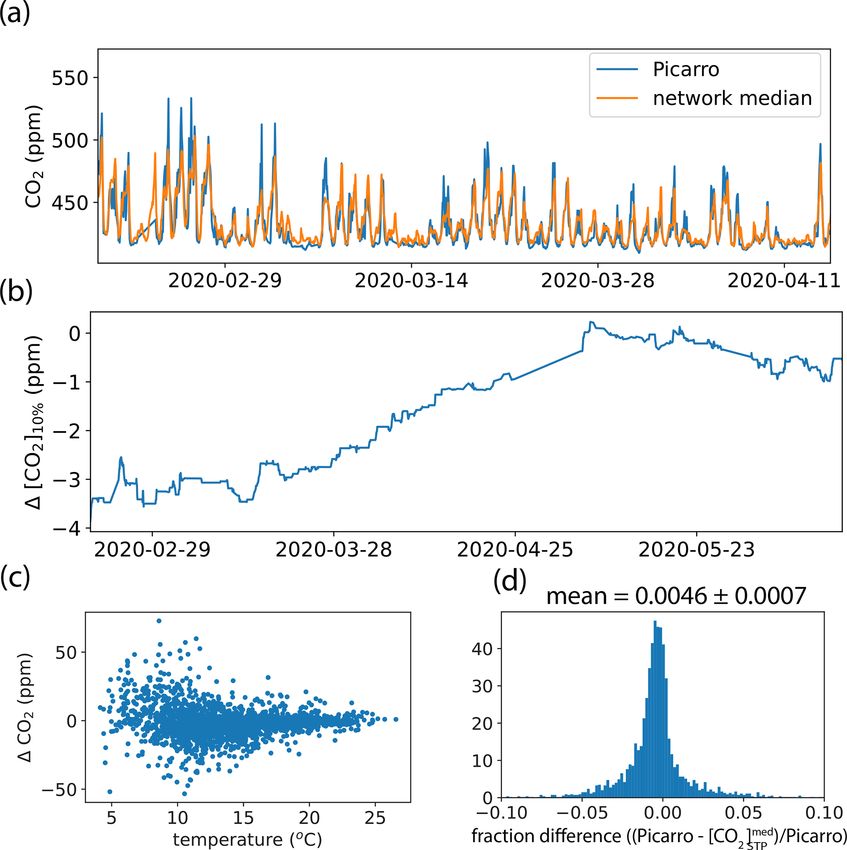
5492               E. R. Delaria et al.: BEACO2 N CO2 measurement accuracy and temperature dependence calibration

Figure 4. (a) CO2 mixing ratios measured by the Picarro instrument at the Richmond Field Station (blue solid), uncorrected CO2 measured
at Elsa Widenmann Elementary School (orange solid), and node temperature measured at Elsa (green dashed). (b) CO2 mixing ratios at Elsa
Widenmann Elementary School with no temperature correction (green), temperature correction applied (green) and measured with a Picarro
instrument at the Richmond Field Station (blue). (c) Temperature dependence at Elsa Widenmann Elementary School of 1 [CO2 ]T10 % .

3   Evaluation of calibration                                         14 April 2020), while preserving local signals (e.g., 15 June
                                                                      2018) (Fig. 6a). The correction is also effective for the data
                                                                      record before deployment of the Picarro reference instrument
Figures 5b, e, and 4c show the temperature dependence of
1 [CO ]T                                                              in August 2017, when the Exploratorium CO2 Buoy, located
       2 10 % nodes located at EBMUD, Montclair, and Elsa
                                                                      in the San Francisco Bay, was used as a reference instrument
Widenmann, respectively. Figures 5a, d, and 4b show a com-
                                                                      (Fig. 6a). The correction of the CO2 diurnal cycle at Laney
parison of the data at EBMUD, Montclair, and Elsa, re-
                                                                      College is most notable during 2017, although midday levels
spectively, with and without adjustment for a temperature-
                                                                      of CO2 are reduced in the corrected data for 2018 and 2020
dependent zero offset. With the application of the tempera-
                                                                      as well (Fig. 6c).
ture correction, the magnitudes of the diurnal cycles are re-
                                                                         The temperature correction method was further validated
duced and demonstrate much better agreement in amplitude
                                                                      by examining neighboring sites in two regions of the Bay
and phase with the Picarro instrument. The resulting diurnal
                                                                      Area during and before periods of high CO2 during Septem-
cycle at EMBUD shows a much more typical diurnal cycle
                                                                      ber 2020 northern California fires. The Richmond sites
for an urban site, with a maximum occurring at mid-morning
                                                                      of Washington Elementary School, Nystrom Elementary
(Fig. 5c). At Montclair, the magnitude of the diurnal cycle
                                                                      School, Dejean Middle School, and Peres Elementary and the
is reduced, reaching a maximum of ∼ 430 ppm CO2 during
                                                                      Vallejo sites of Beverly Hills Elementary School, Mare Is-
the early morning, and a minimum of ∼ 412 ppm CO2 during
                                                                      land Health and Fitness Academy, Grace Patterson Elemen-
midday–a pattern much more aligned with the diurnal cycle
                                                                      tary School, and Highland Elementary School were com-
exhibited at CPS (Figs. 3b, 5c).
                                                                      pared. The resulting temperature-dependent percent differ-
   Following confirmation of the effectiveness of the temper-
                                                                      ences of CO2 between adjacent sites are reduced to approx-
ature correction method on the sensors deployed at EBMUD
                                                                      imately 0 %–2 % from 1 %–5 % (Figs. S3, S6). Temperature
in 2020 (EBMUD 2020, hereafter sensors will be referred to
                                                                      corrections also result in better agreement in CO2 mixing ra-
with the name and site year) and Montclair 2018, we exam-
                                                                      tios between adjacent sites in Richmond (Figs. 7 and S2) and
ined the temperature-corrected CO2 data at the Laney Col-
                                                                      in Vallejo (Figs. S4, S5). The results were identical when a
lege BEACO2 N site during the spring (March–June) of three
                                                                      multiplicative correction term, rather than additive, was con-
different years when different Vaisala CarboCap GMP343
                                                                      sidered (e.g., if the temperature effect was assumed to be on
instruments were deployed. Given the hypothesis that the
                                                                      the CO2 signal magnitude rather than entirely on the instru-
observed temperature dependence is due to temperature-
                                                                      ment zero).
dependent errors in the Vaisala CO2 signal, a successful cal-
ibration should be sensor specific, rather than site specific.
Figure 6b demonstrates the varying 1 [CO2 ]T10 % temperature          Comparison of nearest-neighbor sites
dependence during three different years with different instru-
ment deployments. Each deployment has a distinct offset and           To assess the improvement in the network precision follow-
slope of 1 [CO2 ]T10 % vs. temperature. During all deployment         ing application of the temperature-dependence correction,
years, the temperature correction results in better agreement         we combined observations from the entire Bay Area net-
between the reference instruments and the Vaisala data (e.g.,         work using data from all of 2020. All sites with available

Atmos. Meas. Tech., 14, 5487–5500, 2021                                                https://doi.org/10.5194/amt-14-5487-2021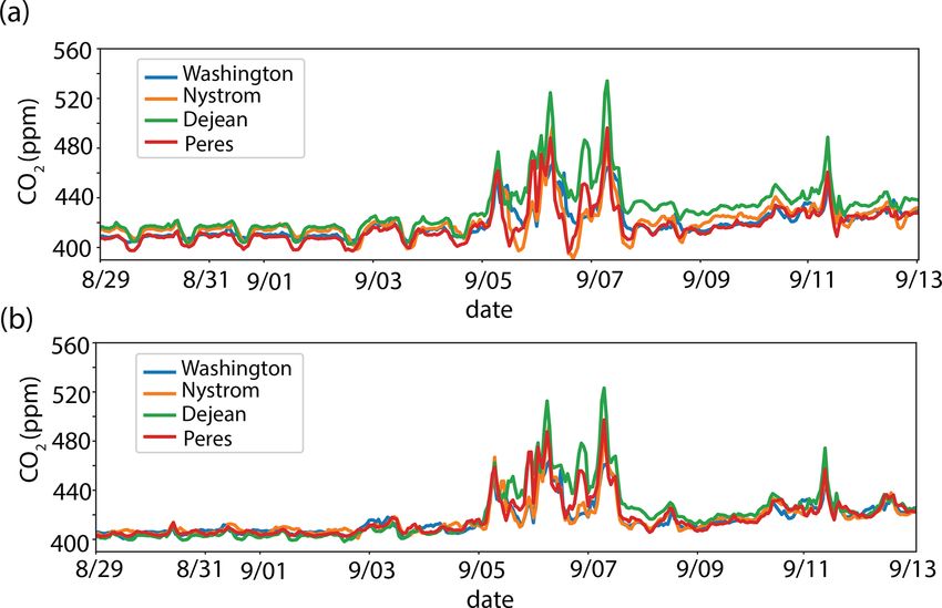
E. R. Delaria et al.: BEACO2 N CO2 measurement accuracy and temperature dependence calibration                                         5493

Figure 5. CO2 mixing ratios at (a) EBMUD and (d) Montclair with no temperature correction (orange), temperature correction applied
(green), and measured with a Picarro instrument at the Richmond Field Station supersite (blue). Temperature dependence of 1 [CO2 ]T10 % at
(b) EBMUD and (e) Montclair. Diurnal cycle with and without temperature correction at (c) EBMUD and (f) Montclair.

Figure 6. Data from 2017 are in top panels, 2018 are in middle panels, 2020 are in bottom panels. (a) CO2 mixing ratios at Laney College
with no temperature correction (green), temperature correction applied (blue), and measured with a Picarro instrument at the Richmond Field
Station supersite (2018 and 2020) or with the Exploratorium Buoy (2017). (b) Temperature dependence at Laney College of 1 [CO2 ]T10 % .
(c) Laney College diurnal CO2 cycle with (green) and without (orange) temperature correction.

data for more than one month of 2020 were included. Near-               culated as: ([CO2 ]X − [CO2 ]Y )/[CO2 ]X . This was
est neighbor pairs of each site were identified, where nearest          done using both the measurements before and after
neighbors to an individual site were considered as the closest          correction
                                                                                     for temperature-dependent
                                                                                                                        instrument zero
BEACO2 N sites within a 2 km radius of the site. There are                      drift               T ,drift
                                                                          [CO2 ]corrected and [CO2 ]corrected . Figure 8a and d show
53 unique nearest neighbor pairs.                                       the fractional differences of each nearest neighbor pair as a
   For each nearest neighbor pair X and Y , an array                    histogram calculated using [CO2 ]drift                    T ,drift
of the fractional differences between sites was cal-                                                          corrected and [CO2 ]corrected ,

https://doi.org/10.5194/amt-14-5487-2021                                                   Atmos. Meas. Tech., 14, 5487–5500, 2021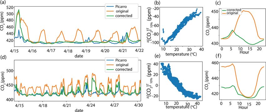
5494                  E. R. Delaria et al.: BEACO2 N CO2 measurement accuracy and temperature dependence calibration

Figure 7. CO2 mixing ratios during and before 2020 September
wildfires at four adjacent sites in Richmond without (a) and with (b)
temperature correction.

respectively. Most nearest neighbor site pairs exhibit a
distribution of fractional differences centered close to zero,
                                                                             Figure 8. Histogram of the fractional differences between nearest
with both positive and negative tails (Fig. 8a, d). The
                                                                             neighbors sites (a) without and (d) with the temperature correction
temperature correction results in a clear improvement of                     applied. Different colors represent different pairs of neighboring
agreement between nearest neighboring sites, with the mean                   sites. Histogram of the fractional differences between all aggregated
of the absolute value of the average fractional differences of               nearest neighboring sites (b) without and (e) with the temperature
all nearest neighbor pairs decreasing by a factor of 2 from                  correction applied fit to a Lorentz distribution. Network mean of the
0.025 to 0.013. For [CO2 ]Tcorrected
                                 ,drift
                                          , this represents an average       percent difference for each nearest neighbor pair averaged by 2 ◦ C
difference of 6.5 ppm at [CO2 ] = 500 ppm. Figure 8b and e                   bins (c) without and (f) with temperature correction applied.
express the fractional differences of nearest neighbor pairs
as a single distribution calculated using [CO2 ]drift      corrected and
       T ,drift
[CO2 ]corrected , respectively. Fit to a Lorentz distribution,               percent differences on temperature. The mean percent differ-
the mean and scale parameter of the distribution of nearest                  ence at all temperatures is also reduced.
neighbor pairs using [CO2 ]drift    corrected is 0.0026 and 0.014,
respectively, without accounting for temperature dependence                  4   Assessment of the network error
and there is a substantial narrowing of the distribution,
resulting in a mean and scale parameter of 0.005 and                         Turner et al. (2016) suggested that a mismatch error of
0.007, respectively, after accounting for the effect of a                    ∼ 1 ppm CO2 would be compatible with relevant constraints
temperature-dependent offset.                                                on point, line, and area CO2 sources of 147, 45, and 9 t C h−1 ,
   Further analysis was performed to confirm that the tem-                   respectively. Minimizing the network measurement error to
perature correction method eliminates any temperature-                       close to 1 ppm is desirable, as at this measurement uncer-
dependent disagreement between nearest neighboring sites.                    tainty, the error in emissions estimates from inverse mod-
The nearest neighbor fractional differences of CO2 data were                 eling becomes dominated by model uncertainties (Turner
separated into 2 ◦ C temperature bins. For each temperature                  et al., 2016). Assessing network error in the field is, how-
bin, the absolute value of the mean fractional difference be-                ever, a complex problem. We approach the problem by ex-
tween each nearest neighbor pair, using either [CO2 ]drift       corrected   ploring differences between adjacent nodes, which should be
or [CO2 ]Tcorrected
             ,drift
                     , was calculated. We then averaged the mean             an upper limit to the uncertainty. Although the site-to-site
fractional difference in each temperature bin over all nearest               variation is strongly influenced by local emissions sources,
neighbor pairs. A plot of the resulting network mean per-                    there are also strong correlations with changes in urban-,
cent difference vs. temperature is shown in Fig. 8c and f, us-               synoptic-, and global-scale CO2 signals that are spatially co-
                                  T ,drift
ing [CO2 ]drift
             corrected and [CO2 ]corrected data, respectively. In the        herent across pairs of adjacent nodes. Variances between ad-
original data, the mean percent differences were greatest at                 jacent nodes are due to a combination of true site-specific
both high and low temperatures. In the temperature-corrected                 signals and instrument biases. It is therefore difficult to know
data, there is no clear dependence of nearest neighbor mean                  the minimum variance in adjacent nodes for a hypothetical

Atmos. Meas. Tech., 14, 5487–5500, 2021                                                        https://doi.org/10.5194/amt-14-5487-2021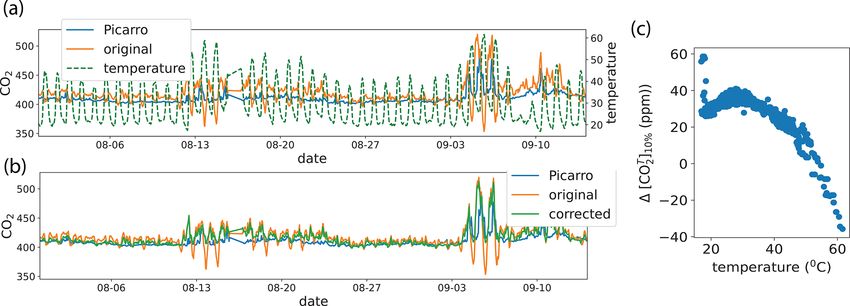
E. R. Delaria et al.: BEACO2 N CO2 measurement accuracy and temperature dependence calibration                                    5495

                                                                       temperature-correction results in a maximum root semivari-
                                                                       ance of 5.5 ± 2 ppm (reduced from 8 ppm in the uncor-
                                                                       rected data). Extrapolated to a distance of zero, the tempera-
                                                                       ture correction method has a predicted root semivariance of
                                                                       1.3 ± 0.9 ppm, representing the network error. This analysis
                                                                       suggests that the temperature correction method provides a
                                                                       meaningful reduction of network measurement uncertainties
                                                                       toward our desired ∼ 1 ppm network error.
                                                                          Length scales for correlations (r 2 ) between sites calculated
                                                                       by Shusterman et al. (2018) during the summer 2017 were
                                                                       larger than the 1.2 km length scale identified here for root
                                                                       semivariance (1.7 km for semivariance). To more directly
                                                                       compare, we also performed the method of Shusterman et al.
                                                                       (2018) on the temperature-corrected CO2 data for the sum-
Figure 9. Semivariogram of BEACO2 N sites for data with temper-
                                                                       mer of 2020. We examined the correlation of CO2 concentra-
ature correction applied. Data are averaged by 0.1 km bins. Plot in-
cludes data from the Picarro instrument at Richmond Field Station.
                                                                       tions for every pairing of Bay Area sites during this period for
                                                                       all hours, during the day, and during the night (Fig. S7). The
                                                                       e-folding distance for the decay of r 2 correlation coefficients
“perfect” measurement. For nearest neighbor sites, the ma-             was 2.8 km for all times, 3.7 km during the day, and 2.8 km
jority of the CO2 signal should show near-zero difference,             at night. This is in good agreement with the length scales
representing the background signal. In the observation record          of 2.9 km at all times, 3.6 km during the day, and 2.2 km at
we would also expect moments when either site in a pair has            night found by Shusterman et al. (2018). The base-line cor-
a larger signal, driven by local emission sources and meteo-           relation for sites separated by more than 20 km was found
rology. Sites closer to the highway also typically have larger         to be 0.46, larger than the correlation background of ∼ 0.3
CO2 signals (Shusterman et al., 2018). In the following sec-           of Shusterman et al. (2018). The temperature correction does
tion we describe a procedure for evaluating network error              not affect the characteristic length scale of BEACO2 N sites,
and summarize the improvements following inclusion of the              but improves the overall base-line correlations and variances.
temperature correction described above.
                                                                       4.2   Contribution of instrument error to site variance
4.1   Site variance and correlation length scales
                                                                       We can represent the network instrument error also by exam-
To evaluate the network error, a semivariogram of γnn vs. dis-         ining the sources contributing to the semivariance between
tance was constructed for [CO2 ]Tcorrected
                                    ,drift
                                           (Fig. 9). Using data        nearest neighboring sites. The semivariance (γnn ) of nearest
from all sites with more than three days of available data dur-        neighboring sites can be expected to have contributions from
ing the summer of 2020, we calculated the semivariance be-             both “true” variations in emissions and meteorology and er-
tween CO2 measurements at each BEACO2 N node, i, and all               roneous differences caused by instrument error. “True” varia-
other sites in the Bay Area network (Eq. 9)                            tions in emissions and meteorology are reflected in temporal
       PN                      2                                      changes in CO2 concentrations due to emissions plumes and
          j [CO2 ]i − [CO2 ]j                                          changes in wind speed and direction. Here we used temporal
γnn =                             .                         (9)
                   2N                                                  changes in CO2 concentrations at a certain site as a proxy for
Summer months were chosen because the average and diur-                “true” atmospheric variations in CO2 . To estimate the portion
nal variability of CO2 mixing ratios are reduced, meaning              of the semivariance resulting from atmospheric phenomena,
that measured site variances are relatively more influenced            an analogous quantity for the hourly variations in CO2 was
by instrument error, rather than by “true” atmospheric vari-           calculated for each site according to Eq. (10):
ance, than in the winter. In Fig. 9 the square root of the                      1 N−1
                                                                                  X
semivariance is plotted against the distance separating the            γhh =          ([CO2 ]h − [CO2 ]h+1 )2 ,                    (10)
                                                                               2N 1
BEACO2 N nodes and fitted with an exponential model. The
Picarro reference instrument at the Richmond Field Station             where N is the number of hours of data and [CO2 ]h , and
was included in this analysis.                                         [CO2 ]h+1 are the measured mixing ratios of CO2 at each
   Using the root semivariance as a correlation metric, in             hour and 1 h later, respectively. The individual instrument er-
temperature-corrected data, the e-folding length scale for             ror was then calculated as:
variation is 1.2 ± 0.3 km (1.7 ± 0.7 km using semivariance as                 √
                                                                       inst = γnn − γhh .                                       (11)
a correlation metric, not shown), supporting the BEACO2 N
hypothesis that 2 km node spacing in a dense network                   The resulting upper-bound instrument error from the median
will capture important elements of local variability. The              of individual instrument errors for the Bay Area network is

https://doi.org/10.5194/amt-14-5487-2021                                                 Atmos. Meas. Tech., 14, 5487–5500, 2021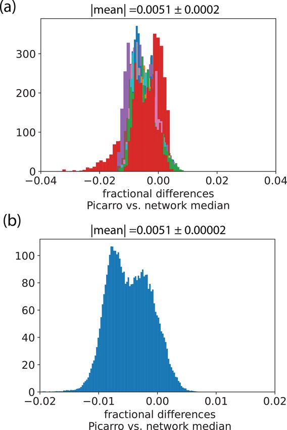
5496                E. R. Delaria et al.: BEACO2 N CO2 measurement accuracy and temperature dependence calibration

2.5 ± 0.5 ppm. (This estimate for nontemperature corrected
data is 4.5 ± 0.9 ppm). We consider this an upper bound be-
cause hourly variations in the CO2 signal reflects the atmo-
spheric changes at an individual site, which may not match
with the atmospheric changes at the nearest neighbor sites.
Variations in emissions or wind velocity may result in larger
“true” differences between a site and its nearest neighbor
than are represented by the site’s hourly variability.
   To reduce the influence from short-term atmospheric vari-
ations, the network error was also estimated using an individ-
ual site’s root mean squared error (RMSEi ) as a metric for
“true” atmospheric variation (Eq. 12) and a “paired” RMSE
(RMSEpaired ) using the mean CO2 signal of its nearest neigh-
bor site (nn [CO2 ]) as a measure of total variation (Eq. 13).
The site error was then calculated according to Eq. 14:
           s
               PN
                h=1   [CO2 ]h − [CO2 ]i
RMSEi =                                                   (12)
                         N
               s
                    PN
                      h=1   [CO2 ]h − nn [CO2 ]
RMSEpaired =                                              (13)
                                N
       q                                                          Figure 10. (a) CO2 mixing ratios measured by the Picarro instru-
inst = RMSE2paired − RMSE2i .                            (14)    ment at the Richmond Field Station (blue) and the median CO2 of
                                                                  all Bay Area nodes having a temperature-dependent slope less than
The resulting network instrument errors were between 0.5          an absolute value of 1 ppm ◦ C−1 (orange). (b) The difference in the
and 4 ppm, with a median of 1.6 ± 0.4 ppm, in good agree-         tenth percentile of CO2 mixing ratios measured by the Picarro in-
ment with the error calculated from the semivariogram fit.        strument and the network median plotted versus date and (c) versus
                                                                  temperature. (d) Histogram of the fractional differences between Pi-
Based on these analyses, we estimate the network error of
                                                                  carro CO2 mixing ratios and the network median. Data for (c) and
the Bay Area BEACO2 N network to be less than 1.6 ppm,            (d) include all of 2020.
close to our goal of 1 ppm network error.

                                                                  calculated for the determination of 1 [CO2 ]T10 % :
5   Application to other city networks
                                                                  1
                                                                      [CO2 ]T10 % =Vaisala [CO2 ]T10 % −med [CO2 ]T10 % .        (15)
The BEACO2 N network has recently been extended to sev-
eral other cities, and will further expand to additional loca-    5.1     Bay Area tests
tions in coming years. Currently, locations where BEACO2 N
nodes are deployed (in addition to the Bay Area) are Hous-        We observe good agreement between the Picarro refer-
ton (19 nodes, network start November 2017), Glasgow in           ence instrument during 2020 and [CO2 ]medSTP (Fig. 10). The
collaboration with the University of Strathclyde (> 20 nodes,     mean percent difference considering all 2020 data is 0.46 %,
network start May 2021), New York City (8 nodes, network          representing an accuracy error of 2 ppm at 420 ppm CO2
start April 2018), and Los Angeles, in collaboration with the     (Fig. 10d). We also do not see evidence of a temperature-
University of Southern California (12 nodes, network start        dependent offset between the Picarro reference instrument
May 2021). The goal of the network is to be self-calibrated,      and [CO2 ]med
                                                                             STP .
as not all locations at which the nodes will be deployed have        The precision of the Bay Area network is negligibly af-
a highly precise and frequently calibrated reference instru-      fected when the network median is used as the reference,
ment. As such, an alternative method of obtaining a refer-        with the mean of the absolute value of the average frac-
ence for the determination of drift, offset, and temperature      tional differences of all nearest neighbor pairs equal to
dependence is needed.                                             0.015 ± 0.008 (compared to 0.013 ± 0.007 with the Picarro
   We find that the network median [CO2 ]STP [CO2 ]med

                                                          STP     as reference) (Fig. S8). The resulting maximum root semi-
can be used as a reference.   To begin, we define the network     variance is 5.5 ± 2 ppm and extrapolated root semivariance
median [CO2 ]med

                 STP   as the median [CO2 ]STP of sites having    at 0 km separation is 0.8 ± 0.9 ppm, respectively, approxi-
a temperature-dependent slope (mT ) less than 1 ppm ◦ C−1 .       mately equal to the values calculated when the Picarro is
[CO2 ]med
       STP is used as a “reference site” from which               used as a reference. The network accuracy is however, more
temperature-based 10th percentile data med [CO2 ]T10 % is

                                                                  appreciably altered. Figure 11 shows the fractional differ-

Atmos. Meas. Tech., 14, 5487–5500, 2021                                                https://doi.org/10.5194/amt-14-5487-2021
E. R. Delaria et al.: BEACO2 N CO2 measurement accuracy and temperature dependence calibration 5497
Figure 12. Fractional difference between the Bay Area network me-
dian calculated from all Bay Area sites and the network median
calculated from a subset of between one and 26 nodes. A random
subset of n = 1–26 nodes were selected to calculate the mean frac-
tional difference between the network median CO2 and the median
calculated using the subset. This was repeated 100 times for each of
n = 1–26 nodes. The reported fractional difference and error bars
are the average and 95 % confidence interval of the mean fractional
difference from the 100 random samples.
Bay Area. To use [CO2 ]medSTP as a reference, we must have suf-
ficient nodes from which to calculate the network median. To
Figure 11. (a) Histogram of the fractional differences between sites evaluate this, for n = 1–26, a random subset of n Bay Area
with temperature-corrected CO2 calculated using the Picarro instru- nodes was selected 100 times. For each of the 100 random
ment and the Bay Area network median as a reference. Different subsets of n nodes, the mean fraction difference was calcu-
colors represent different sites. The mean indicated is the average lated between the network median CO2 and the median cal-
of the absolute values of each neighboring pair’s mean fractional culated using the subset. The average and standard error of
difference. (b) Histogram of the aggregated fractional differences the 100 mean fraction differences was then calculated. The
between sites with temperature-corrected CO2 calculated using the results of this analysis are presented in Fig. 12. We suggest
Picarro instrument and the Bay Area network median as a reference.
that a minimum of 7 nodes with mT less than 1 ppm ◦ C−1 is
The mean and error indicated are the mean and 95 % confidence in-
required for the accuracy error to be lower than 2 %. For less
terval of the distribution.
than 1 % error, at least 12 nodes are required.
ence between [CO2 ]Tcorrected
,drift
determined using the Picarro and 5.2 Houston
med
[CO2 ]STP as a reference at each site. The resulting mean per-
cent difference is 0.51 ± 0.02 %, representing a network ac- Data from the Houston network were subsequently calibrated
curacy error of 2 ppm at 420 ppm CO2 . This accuracy error using [CO2 ]med
STP as a reference for determining temperature
is mainly driven by small differences in the offsets (2 ppm dependence, drift, and offset. Temperature dependence cali-
on average) and mT (0.2 ppm ◦ C−1 on average, see Supple- bration of each site in the Houston network was performed
ment) between [CO2 ]Tcorrected
,drift
calculated using the Picarro and twice. All sites were first included in [CO2 ]medSTP and sites
med
[CO2 ]STP as a reference. These results suggest that the net- with mT greater than 1 ppm ◦ C−1 were identified. These sites
work precision can be expected to remain near 1 ppm CO2 were then excluded from [CO2 ]med STP and each site was recali-
with the use of [CO2 ]med
STP as a reference, but additional ac- brated. Histograms of the fraction differences between near-
curacy error of 2 ppm may be introduced. The influence of a est neighbor sites are shown in Fig. 13. The average mean
sea breeze in the Bay Area makes the median tenth percentile percent difference between nearest neighbors was 2 ± 1 %.
CO2 measured by Bay Area nodes a regional background. Though considerably larger than the differences between
Although the median tenth percentile of other inland sensor nearest neighbors in the Bay Area network, it is not immedi-
networks may not represent a regional background, it can be ately clear whether this difference is caused by greater pre-
expected to represent the overall network regional average cision error in Houston or differing meteorology and CO2
baseline. sources that cause greater differences between CO2 mixing
Analysis of the Bay Area network was performed on the ratios at adjacent sites. We attempted to perform a similar in-
36 nodes with sufficient data availability for 2020. However, strumental error analysis, but there are currently insufficient
the newly established networks have fewer nodes than in the overlapping CO2 data in Houston for uncertainty analysis.
https://doi.org/10.5194/amt-14-5487-2021 Atmos. Meas. Tech., 14, 5487–5500, 20215498 E. R. Delaria et al.: BEACO2 N CO2 measurement accuracy and temperature dependence calibration
to the network and does not necessarily require a reference
instrument, although the addition of a reference instrument
provides greater network accuracy. The implementation of
the temperature correction method produces more reasonable
diurnal cycles, diurnal cycles that are maintained for sites in-
fluenced by similar emissions sources, and better agreement
between adjacent sites. We additionally describe methods for
characterizing network scale uncertainties and site-to-site bi-
ases. The average variation between adjacent sites was found
to be 1.3 % following implementation of temperature correc-
tion (compared to 2.5 % prior to the correction). The temper-
ature correction greatly improves the precision of CO2 mea-
surements in the BEACO2 N network.
We show that the network precision can be maintained at
1.3 % even in locations without a high-cost reference instru-
ment, using the network median as a reference, provided that
there are at least 12 sites with small temperature dependen-
cies. This has important implications for the expansion of
BEACO2 N to additional cities globally, as well as for other
dense low-cost CO2 networks. However, without a reference
instrument, the network accuracy error increases relative to a
network that utilizes a reference instrument by ∼ ±2 ppm.
Figure 13. (a) Histogram of the fractional differences between near-
est neighbors sites in the Houston network with the temperature cor-
rection applied using the network median as a reference. Different Data availability. The data used for this study are publicly avail-
colors represent different pairs of neighboring sites. The mean in- able at http://beacon.berkeley.edu (Cohen Research, 2021). Raw
dicated is the average of the absolute values of each neighboring data can be given upon request.
pair’s mean fractional difference. The error is the associated 95 %
confidence interval. (b) Histogram of the fractional differences be-
tween all aggregated nearest neighbors sites with the temperature
Supplement. The supplement related to this article is available on-
correction applied. The mean and error indicated are the mean and
line at: https://doi.org/10.5194/amt-14-5487-2021-supplement.
95 % confidence interval, respectively, of the distribution.
Author contributions. JK, HLF, CN, and PJW collected the data
However, we do not have reason to expect the instrument er- used in this analysis. ERD composed the manuscript and designed
rors would be any larger in the Houston network. and executed the analysis in consultation with JK and KW. KW also
aided with data processing and implementation of the temperature
calibration method. JK and RCC provided additional manuscript
6 Conclusions feedback and RCC supervised the project.
We have assessed the accuracy of the BEACO2 N network
following in situ calibration of the temperature-dependence Competing interests. Ronald C. Cohen is associate editor of Atmo-
in Vaisala CO2 sensors. We report meaningful reduc- spheric Measurement Techniques.
tions in network uncertainties following application of a
temperature-dependence correction, and a resulting network
instrument error of 1.6 ppm CO2 or less. Disclaimer. Publisher’s note: Copernicus Publications remains
A method for correcting Vaisala instrument temperature neutral with regard to jurisdictional claims in published maps and
dependence in BEACO2 N has been established and eval- institutional affiliations.
uated using sites across the San Francisco Bay Area net-
work. The method corrects observations from individual in-
Acknowledgements. We also thank Alexander J. Turner for his in-
struments so that they exhibit a temperature dependence in
put and former members of the BEACO2 N project for establishing
their lowest temperature-based 10th percentile of CO2 data
the network: Alexis A. Shusterman, Virginia Teige, and Kaitlyn Li-
that is equivalent to that of a reference site, thus correct- eschke.
ing erroneous instrument temperature dependence while pre-
serving true diurnal cycles and local signals. This field cal-
ibration of temperature dependence can be entirely internal
Atmos. Meas. Tech., 14, 5487–5500, 2021 https://doi.org/10.5194/amt-14-5487-2021E. R. Delaria et al.: BEACO2 N CO2 measurement accuracy and temperature dependence calibration 5499
Financial support. This research has been supported by the Koret Idso, S. B., Idso, C. D., and Balling, R. C.: Seasonal and diurnal
Foundation and University of California, Berkeley. variations of near-surface atmospheric CO2 concentration within
a residential sector of the urban CO2 dome of Phoenix, AZ, USA,
Atmos. Environ., 36, 1655–1660, https://doi.org/10.1016/S1352-
Review statement. This paper was edited by William R. Simpson 2310(02)00159-0, 2002.
and reviewed by two anonymous referees. IPCC: Summary for Policymakers, in: Climate Change 2021: The
Physical Science Basis. Contribution of Working Group I to the
Sixth Assessment Report of the Intergovernmental Panel on Cli-
mate Change, edited by: Masson-Delmotte, V., Zhai, P., Pirani,
A., Connors, S. L., Péan, C., Berger, S., Caud, N., Chen, Y.,
References Goldfarb, L., Gomis, M. I., Huang, M., Leitzell, K., Lonnoy, E.,
Matthews, J. B. R., Maycock, T. K., Waterfield, T., Yelekçi, O.,
Andrews, A. E., Kofler, J. D., Trudeau, M. E., Williams, J. C., Neff, Yu, R., and Zhou, B., Cambridge University Press, in press, 2021.
D. H., Masarie, K. A., Chao, D. Y., Kitzis, D. R., Novelli, P. C., Kim, J., Shusterman, A. A., Lieschke, K. J., Newman, C.,
Zhao, C. L., Dlugokencky, E. J., Lang, P. M., Crotwell, M. J., and Cohen, R. C.: The BErkeley Atmospheric CO2 Ob-
Fischer, M. L., Parker, M. J., Lee, J. T., Baumann, D. D., Desai, servation Network: field calibration and evaluation of low-
A. R., Stanier, C. O., De Wekker, S. F. J., Wolfe, D. E., Munger, cost air quality sensors, Atmos. Meas. Tech., 11, 1937–1946,
J. W., and Tans, P. P.: CO2 , CO, and CH4 measurements from tall https://doi.org/10.5194/amt-11-1937-2018, 2018.
towers in the NOAA Earth System Research Laboratory’s Global Kort, E. A., Angevine, W. M., Duren, R., and Miller, C. E.: Sur-
Greenhouse Gas Reference Network: instrumentation, uncer- face observations for monitoring urban fossil fuel CO2 emis-
tainty analysis, and recommendations for future high-accuracy sions: Minimum site location requirements for the Los An-
greenhouse gas monitoring efforts, Atmos. Meas. Tech., 7, 647– geles megacity, J. Geophys. Res.-Atmos., 118, 1577–1584,
687, https://doi.org/10.5194/amt-7-647-2014, 2014. https://doi.org/10.1002/jgrd.50135, 2013.
Bréon, F. M., Broquet, G., Puygrenier, V., Chevallier, F., Xueref- Lateb, M., Meroney, R., Yataghene, M., Fellouah, H., Saleh,
Remy, I., Ramonet, M., Dieudonné, E., Lopez, M., Schmidt, F., and Boufadel, M.: On the use of numerical mod-
M., Perrussel, O., and Ciais, P.: An attempt at estimat- elling for near-field pollutant dispersion in urban envi-
ing Paris area CO2 emissions from atmospheric concentra- ronments – A review, Environ. Pollut., 208, 271–283,
tion measurements, Atmos. Chem. Phys., 15, 1707–1724, https://doi.org/10.1016/j.envpol.2015.07.039, 2016.
https://doi.org/10.5194/acp-15-1707-2015, 2015. Lauvaux, T., Miles, N. L., Deng, A., Richardson, S. J., Cambal-
Brondfield, M. N., Hutyra, L. R., Gately, C. K., Raciti, S. M., and iza, M. O., Davis, K. J., Gaudet, B., Gurney, K. R., Huang, J.,
Peterson, S. A.: Modeling and validation of on-road CO2 emis- O’Keefe, D., Song, Y., Karion, A., Oda, T., Patarasuk, R., Razli-
sions inventories at the urban regional scale, Environ. Pollut., vanov, I., Sarmiento, D., Shepson, P., Sweeney, C., Turnbull, J.,
170, 113–123, https://doi.org/10.1016/j.envpol.2012.06.003, and Wu, K.: High-resolution atmospheric inversion of urban CO2
2012. emissions during the dormant season of the Indianapolis Flux
Cohen Research: Berkeley Environmental Air-quality & CO2 Net- Experiment (INFLUX), J. Geophys. Res.-Atmos., 121, 5213–
work (BEACO2N), University of California Berkeley, available 5236, https://doi.org/10.1002/2015JD024473, 2016.
at: http://beacon.berkeley.edu, last access: 9 August 2021. Lauvaux, T., Gurney, K. R., Miles, N. L., Davis, K. J., Richard-
Coutts, A. M., Beringer, J., and Tapper, N. J.: Character- son, S. J., Deng, A., Nathan, B. J., Oda, T., Wang, J. A.,
istics influencing the variability of urban CO2 fluxes Hutyra, L., and Turnbull, J.: Policy-Relevant Assessment of Ur-
in Melbourne, Australia, Atmos. Environ., 41, 51–62, ban CO2 Emissions, Environ. Sci. Technol., 54, 10237–10245,
https://doi.org/10.1016/j.atmosenv.2006.08.030, 2007. https://doi.org/10.1021/acs.est.0c00343, 2020.
Fu, P., Xie, Y., Moore, C. E., Myint, S. W., and Bernacchi, C. J.: A Martin, C. R., Zeng, N., Karion, A., Dickerson, R. R., Ren,
Comparative Analysis of Anthropogenic CO2 Emissions at City X., Turpie, B. N., and Weber, K. J.: Evaluation and envi-
Level Using OCO-2 Observations: A Global Perspective, Earth ronmental correction of ambient CO2 measurements from a
Future, 7, 1058–1070, https://doi.org/10.1029/2019EF001282, low-cost NDIR sensor, Atmos. Meas. Tech., 10, 2383–2395,
2019. https://doi.org/10.5194/amt-10-2383-2017, 2017.
Gately, C. K., Hutyra, L. R., Wing, I. S., and Brondfield, McKain, K., Wofsy, S. C., Nehrkorn, T., Eluszkiewicz, J.,
M. N.: A Bottom up Approach to on-Road CO2 Emissions Ehleringer, J. R., and Stephens, B. B.: Assessment of ground-
Estimates: Improved Spatial Accuracy and Applications for based atmospheric observations for verification of greenhouse
Regional Planning, Environ. Sci. Technol., 47, 2423–2430, gas emissions from an urban region, P. Natl. Acad. Sci. USA,
https://doi.org/10.1021/es304238v, 2013. 109, 8423–8428, https://doi.org/10.1073/pnas.1116645109,
Gately, C. K., Hutyra, L. R., Peterson, S., and Sue Wing, I.: Ur- 2012.
ban emissions hotspots: Quantifying vehicle congestion and air Müller, M., Graf, P., Meyer, J., Pentina, A., Brunner, D., Perez-
pollution using mobile phone GPS data, Environ. Pollut., 229, Cruz, F., Hüglin, C., and Emmenegger, L.: Integration and cali-
496–504, https://doi.org/10.1016/j.envpol.2017.05.091, 2017. bration of non-dispersive infrared (NDIR) CO2 low-cost sensors
Gurney, K. R., Mendoza, D. L., Zhou, Y., Fischer, M. L., Miller, and their operation in a sensor network covering Switzerland, At-
C. C., Geethakumar, S., and de la Rue du Can, S.: High mos. Meas. Tech., 13, 3815–3834, https://doi.org/10.5194/amt-
Resolution Fossil Fuel Combustion CO2 Emission Fluxes for 13-3815-2020, 2020.
the United States, Environ. Sci. Technol., 43, 5535–5541,
https://doi.org/10.1021/es900806c, 2009.
https://doi.org/10.5194/amt-14-5487-2021 Atmos. Meas. Tech., 14, 5487–5500, 2021You can also read