Climate change in a conceptual atmosphere-phytoplankton model - ESD
←
→
Page content transcription
If your browser does not render page correctly, please read the page content below
Earth Syst. Dynam., 11, 603–615, 2020
https://doi.org/10.5194/esd-11-603-2020
© Author(s) 2020. This work is distributed under
the Creative Commons Attribution 4.0 License.

                                   Climate change in a conceptual
                                  atmosphere–phytoplankton model
                     György Károly1 , Rudolf Dániel Prokaj2 , István Scheuring3,4 , and Tamás Tél5,6
                    1 Institute
                              of Nuclear Techniques, Budapest University of Technology and Economics,
                                        Műegyetem rkp. 3., 1111 Budapest, Hungary
                     2 Department of Stochastics, Budapest University of Technology and Economics,

                                        Műegyetem rkp. 3., 1111 Budapest, Hungary
       3 MTA-ELTE Theoretical Biology and Evolutionary Ecology Research Group, Department of Plant Taxonomy,

                          Ecology and Theoretical Biology, Eötvös University, Budapest, Hungary
             4 Evolutionary Systems Research Group, MTA Centre for Ecological Research, Tihany, Hungary
                        5 Department of Theoretical Physics, Eötvös University, Budapest, Hungary
                           6 MTA-ELTE Theoretical Physics Research Group, Budapest, Hungary

                                     Correspondence: György Károlyi (karolyi@reak.bme.hu)

                                    Received: 18 November 2019 – Discussion started: 6 December 2019
                                  Revised: 5 June 2020 – Accepted: 22 June 2020 – Published: 16 July 2020

       Abstract. We develop a conceptual coupled atmosphere–phytoplankton model by combining the Lorenz’84
       general circulation model and the logistic population growth model under the condition of a climate change
       due to a linear time dependence of the strength of anthropogenic atmospheric forcing. The following types of
       couplings are taken into account: (a) the temperature modifies the total biomass of phytoplankton via the carrying
       capacity; (b) the extraction of carbon dioxide by phytoplankton slows down the speed of climate change; (c) the
       strength of mixing/turbulence in the oceanic mixing layer is in correlation with phytoplankton productivity. We
       carry out an ensemble approach (in the spirit of the theory of snapshot attractors) and concentrate on the trends
       of the average phytoplankton concentration and average temperature contrast between the pole and Equator,
       forcing the atmospheric dynamics. The effect of turbulence is found to have the strongest influence on these
       trends. Our results show that when mixing has sufficiently strong coupling to production, mixing is able to force
       the typical phytoplankton concentration to always decay globally in time and the temperature contrast to decrease
       faster than what follows from direct anthropogenic influences. Simple relations found for the trends without this
       coupling do, however, remain valid; just the coefficients become dependent on the strength of coupling with
       oceanic mixing. In particular, the phytoplankton concentration and its coupling to climate are found to modify
       the trend of global warming and are able to make it stronger than what it would be without biomass.

1   Introduction                                                        ponent that needs to be included in such conceptual models
                                                                        is the phytoplankton content of the ocean.
Large-scale general circulation models typically take into ac-             Oceans are the major sink for the atmospheric CO2 (Hader
count the interaction of the atmosphere with land vegetation            et al., 2014; Li et al., 2012). CO2 is either stored as dissolved
and marine biomass production in the form of a huge num-                inorganic carbon or transferred to the underlying sediment by
ber of parametrized processes (see, e.g., Marinov et al., 2010;         biological carbon pump. The motor of the biological pump
Zhong et al., 2011; Mongwe et al., 2018; Wilson et al., 2018).          is phytoplankton, which is one of the major components of
A basic understanding of such coupling is, however, easier to           the global carbon cycle, hence influencing decisively atmo-
obtain in low-order conceptual models, where even analytic              spheric CO2 (Hutchins and Fu, 2017; Sanders et al., 2014;
results may be available. Probably the most important com-

Published by Copernicus Publications on behalf of the European Geosciences Union.
604                                      G. Károly et al.: Climate change in a conceptual atmosphere–phytoplankton model

Turner, 2005; Falkowski et al., 2000). Besides, phytoplank-       quantifiers (e.g., expected, average properties) of the climate.
ton is responsible for nearly half of the total primary produc-   Since our information on the actual state of the climate is in-
tion on Earth (Basu and Mackey, 2018). Consequently, it is        complete, one imagines an ensemble of parallel Earth sys-
extremely important to understand the interaction of phyto-       tems carrying parallel climate realizations subjected to the
plankton in oceans with effects contributing to global climate    same set of physical laws, boundary conditions, and external
change. However, the task is very challenging; change in at-      forcing but with different initial conditions. Then the chaotic
mospheric CO2 level can have opposite impacts on processes        or turbulence-like properties of the climate dynamics allows
influencing the phytoplankton and the intensity of the biolog-    for distinct climate realizations (for a review, see Tél et al.,
ical carbon pump. Increased atmospheric CO2 level increases       2019). These realizations, however, cannot be arbitrary, since
ocean temperature, decreases pH, increases water stratifica-      only those that are compatible with physical laws and the
tion, and influences general oceanic circulation. These can       given forcing are permitted. The ensemble of realizations de-
all modify the net productivity and the composition of phyto-     fines a probability distribution of all the relevant variables at
plankton and can have either a positive or negative net effect    any instant of time from which one can obtain expected en-
on the biological carbon pump (Basu and Mackey, 2018, and         semble average properties of the climate (for more details,
references therein).                                              and mathematical aspects, see Sect. 5).
   In spite of the current trend to include biogeochemistry          It is therefore natural to use the ensemble view in our
in climate models (see, e.g., Schlunegger et al., 2019), a        conceptual biogeochemistry model, too. The ensemble ap-
basic understanding of such processes is still limited. It is     proach in it corresponds to generating parallel atmosphere–
still under debate whether net primary production is increas-     phytoplankton realizations from different initial conditions.
ing or decreasing in coupled carbon–climate models as a           In our model, the number of variables is four; hence the snap-
consequence of warming-induced production increase and            shot attractor in the full state space is difficult to visualize.
stronger nutrient limitations induced by increased stratifi-      We therefore concentrate on ensemble averages, and the in-
cation (Laufkötter et al., 2015). The situation appears to        ternal variability will be expressed in terms of variances. We
be similar to the understanding of thermal or fluid dy-           include, in a simple heuristic form, important feedbacks in
namical concepts decades ago. The study of, e.g., the en-         the model: (a) the change in the atmospheric temperature
ergy balance (Ghil, 1976) or the thermohaline circulation         that modifies phytoplankton concentration; (b) the extrac-
(Stommel, 1961) started with elementary conceptual mod-           tion of CO2 by phytoplankton; and (c) wind energy that en-
els which later evolved into more complex ones and are by         hances the strength of turbulence in the oceanic mixing layer,
now decisive components of cutting-edge climate models.           which increases the phytoplankton production (Estrada and
We therefore propose here to study a conceptual atmosphere–       Berdalet, 1997; Peters and Marrasé, 2000; Jäger et al., 2010).
phytoplankton model where emphasis is on a proper choice             The paper is organized as follows. In Sect. 2 we describe
of couplings (feedbacks). Thus, in our model, an increase in      the model and define the relevant coupling parameters. With-
the global temperature affects the global primary production      out mixing, exact relations can be derived. The most impor-
of ocean. As we emphasize above, phytoplankton plays sig-         tant of these are summarized in Sect. 3, while details of the
nificant role in the global CO2 balance (De La Rocha and          calculations are relegated to Sect. S1 in the Supplement . In
Passow, 2014; Falkowski, 2014; Guidi et al., 2016); hence         the presence of mixing, numerical simulations are carried out
our aim is to take an elementary description of phytoplank-       in the spirit of snapshot attractors. The results are summa-
ton dynamics coupled to an elementary model of the atmo-          rized in Sect. 4 where one learns that the extraction effect of
sphere. The direct effect of increased CO2 concentration on       CO2 has the least influence on the general behavior in the
phytoplankton dynamics can be stimulating or inhibiting; we       presence of mixing. The feedback of the temperature con-
study both scenarios. As atmospheric model, we use Lorenz’s       trast on the phytoplankton concentration has important con-
elementary global circulation model (Lorenz, 1984), which         sequences, but these are suppressed by a sufficiently strong
was extended to mimic climate change (Drótos et al., 2015).       mixing, which converts the typical phytoplankton concen-
The global phytoplankton concentration is represented by a        tration to always decay in time, and surprisingly, the typi-
simple logistic model in which the carrying capacity is cou-      cal temperature contrast is found to decrease faster than that
pled with the CO2 content (direct effect) depending also on       solely by direct anthropogenic effects. Planar sections of the
the concentration itself and on the wind energy influencing       4-dimensional snapshot attractor underlying the dynamics
the oceanic mixing layer (indirect effect of climate change).     are presented in Sect. 5, and our conclusions are drawn in
   An appropriate treatment of even elementary models de-         Sect. 6. Additional figures are presented in Sect. S2 in the
scribing climate change is not obvious, since basic param-        Supplement . A list of variables and parameters is given in
eters change with time, and, therefore, traditional long-time     Sect. S3, while Sect. S4 contains a sample of the C code ap-
averages cannot be used to define (in the sense of any sta-       plied during numerical simulations.
tistical quantifiers) a state of the climate. An emerging new
view, already embraced by Drótos et al. (2015), follows a dif-
ferent route to obtain information on instantaneous statistical

Earth Syst. Dynam., 11, 603–615, 2020                                                https://doi.org/10.5194/esd-11-603-2020
G. Károly et al.: Climate change in a conceptual atmosphere–phytoplankton model                                                605

2   The model                                                        This latter choice will be kept throughout the paper. The as-
                                                                     sumption of Eq. (2) for the global phytoplankton dynamics
The physical content of Lorenz’s atmospheric circulation             tacitly implies that phytoplankton biomass determines the to-
model for the midlatitudes (Lorenz, 1984, 1990) on one               tal biomass of the oceans and also that no catastrophic events
hemisphere is the following. The main forcing is the temper-         (no mass extinction or invasion of species) can take place in
ature difference Te − Tp between the Equator and the pole.           this model.
This is proportional to model variable F influencing most di-           A basic feature of the observed climate change on Earth
rectly the wind speed of the Westerlies represented by x. As         is that the polar temperature Tp (t) increases, while the equa-
an effect of baroclinic instability, cyclonic activity facilitates   torial one Te remains practically constant (Serezze and Fran-
poleward heat transport, two modes of which are represented          cis, 2006; Blunden and Arndt, 2013). We can thus write in
by y and z. The model reads as follows:                              suitable units the temperature contrast parameter as F (t) =
                                                                     Te −Tp (t). The mean temperature in these units is then T (t) =
ẋ = −y 2 − z2 − ax + aF (t),                                (1a)
                                                                     (Te + Tp (t))/2 = Te − F (t)/2. We are interested in dominant,
ẏ = xy − bxz − y + G,                                       (1b)    leading-order effects and assume therefore the carrying ca-
ż = xz + bxy − z.                                           (1c)    pacity to be coupled linearly by a small coupling constant
                                                                     to the mean temperature relative to some reference state of
For the parameter setting we take the common choice: a =             mean temperature Tr , in which the temperature contrast pa-
1/4, b = 4, and G = 1. The equations appear in a dimension-          rameter is Fr = 2(Te −Tr ). The temperature difference T −Tr
less form with the time unit corresponding to 5 d.                   is then −(F − Fr )/2. We therefore write
   By using time-dependent forcing, F (t), as Drótos et al.
(2015), we also model the contribution of the varying CO2            K(t) = Kr − α (F (c(t), t) − Fr ) ,                        (3)
content in association with the greenhouse effect. Besides
                                                                     where Kr is the carrying capacity in the reference state char-
the variation in CO2 due to effects appearing in F (t), the
                                                                     acterized by Fr . Coefficient α represents coupling (a) be-
extraction of CO2 by phytoplankton is also included into
                                                                     tween the carrying capacity K and climate change, repre-
our model. The CO2 content stored in marine ecosystems or
                                                                     sented by F , and shall be called the enrichment parameter;
buried in the seabed is correlated with primary production
                                                                     see Fig. 1 where the full set of feedbacks considered in the
(Falkowski et al., 1998, 2003). Thus, as discussed in the In-
                                                                     model is schematically presented. This coupling may be ei-
troduction, modeling the interaction of phytoplankton and at-
                                                                     ther positive or negative. For example, increased CO2 level
mospheric dynamics is a good proxy for the studying marine
                                                                     enhances the efficiency of photosynthesis (α > 0); however,
ecosystem interaction with atmospheric dynamics. Hence,
                                                                     acidification because of increased CO2 levels depresses res-
we couple the Lorenzian atmospheric dynamics to that of
                                                                     piration (α < 0) (Reid et al., 2009; Mackey et al., 2015). Sim-
the photosynthesizing oceanic biomass, assumed to be dom-
                                                                     ilarly, increased water temperature can have both a positive
inated by phytoplankton of concentration c(t). The tempera-
                                                                     and negative effect on phytoplankton biomass in different re-
ture contrast parameter thus also depends on the global phy-
                                                                     gions of Earth (Chust et al., 2014; Roberts et al., 2017). We
toplankton concentration c: F (t) → F (c(t), t), with a form to
                                                                     shall, therefore, allow for both positive and negative values
be given below.
                                                                     of α with |α| small.
   Spatial inhomogeneities in nutrient and consequently phy-
                                                                        Phytoplankton dynamics influences the temperature con-
toplankton content due to, e.g., oceanic eddies and up-
                                                                     trast. If concentration c increases, the temperature contrast
wellings are known to play an important local role in nature.
                                                                     F increases, too, because the biomass extracts more CO2 .
However, a global atmospheric model like Eq. (1) can ade-
                                                                     In leading order, we therefore express the concentration-
quately be coupled only to a global phytoplankton dynamics
                                                                     dependent temperature contrast parameter as a linear func-
model. Therefore, the concentration itself is assumed in this
                                                                     tion of the concentration:
simple setup to follow a logistic population growth
                                                                   F (t) = F (c(t), t) = β(c(t) − cr ) + F0 (t),              (4)
               c
ċ = rc 1 −          .                                      (2)
              K(t)                                                   with a small β > 0, where cr is the phytoplankton concen-
                                                                     tration in the reference state. Coefficient β represents cou-
Carrying capacity K is taken to depend on the average tem-           pling (b) due to the extraction of CO2 by phytoplankton, and
perature of the hemisphere or, equivalently, on the tempera-         we therefore call β the extraction parameter (see Fig. 1). The
ture contrast F . As a consequence, K depends on time also           second term, F0 (t), represents the primary external forcing
via the concentration c: K(t) = K(c(t), t). We shall see that        due to the CO2 content of anthropogenic origin. The increase
an important oceanic effect, that of the turbulence in the mix-      in both F0 and (c(t) − cr ) leads to an increase in the temper-
ing layer, can be incorporated into carrying capacity K, al-         ature contrast F (t). With this form of F the carrying capac-
though only on a global scale. Parameter r sets the growth           ity (3) is
rate of the phytoplankton. If, e.g., r = 1, the phytoplankton
characteristic time is 5/r = 5 d, as that of the atmosphere.         K(t) = Kr − α [β (c(t) − cr ) + F0 (t) − Fr ] .            (5)

https://doi.org/10.5194/esd-11-603-2020                                                  Earth Syst. Dynam., 11, 603–615, 2020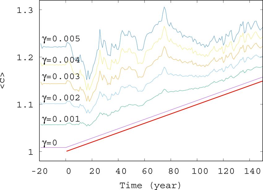
606                                         G. Károly et al.: Climate change in a conceptual atmosphere–phytoplankton model

                                                                          We can model seasonality, too, as Lorenz also did (Lorenz,
                                                                        1990), by augmenting Eq. (6) with a periodic term as follows:

                                                                        F0 (t) = Fr − D0 t + A sin(ωt).                             (8)

                                                                        His choice was A = 2 with ω = 2π/73, which we shall
                                                                        adopt. Our climate change starts with year 0, and this year
                                                                        begins at the time instant t = 0. Note that this time instant
                                                                        belongs to an autumnal equinox according to Eq. (8), and,
                                                                        furthermore, Fr − D0 t can be considered as the annual mean
                                                                        temperature contrast. Any time t mod 73 = 0 coincides with
                                                                        other autumnal equinoxes, and results will be presented on
                                                                        this day of the year throughout the paper.
                                                                           Up to this point, the atmospheric variables have not en-
                                                                        tered the concentration dynamics. Without the linear and
Figure 1. Sketch of the feedbacks considered in the model. Tem-         constant terms (representing dissipation and forcing, respec-
perature contrast F0 between the pole and the Equator, containing       tively), Eq. (1) would conserve the total kinetic energy
also seasonal variability, is augmented by anthropogenic effects D0 .
The main interactions are (α) the enrichment effect of atmospheric      E = ẋ 2 + ẏ 2 + ż2
temperature on phytoplankton, (β) the extraction of CO2 by phyto-
plankton, and (γ ) oceanic mixing, driven by atmospheric dynamics,      of the atmosphere. From the point of view of the biomass,
affecting phytoplankton productivity.
                                                                        it is natural to assume that the activity of the atmosphere
                                                                        influences the ocean dynamics within its uppermost mixing
   Without a restriction of generality, we can choose the ref-          layer (Sverdrup, 1953; Whitt et al., 2017), in particular, the
erence carrying capacity to be Kr = 1, implying a reference             strength of turbulence, and hence the depth of mixing layer.
concentration cr = 1. This choice only rescales parameters α            Note that component ẋ 2 represents the contribution of zonal
and β in Eqs. (3) and (4), respectively.                                winds to the total atmospheric energy, while ẏ 2 + ż2 rep-
   Starting from negative times, we assume the Earth system             resents wind energy stemming from cyclonic activity. The
to be in climatic and population dynamical equilibrium up to            depth of the mixing layer and, consequently, the carrying ca-
time t = 0. This state, chosen as the reference state, is charac-       pacity are assumed to increase linearly with E in our model,
terized by a time-independent mean temperature Tr , concen-             with a small coupling constant. The most general form of the
tration cr = Kr , and F0 (t) = Fr . At time zero, climate change        carrying capacity K is thus
sets in expressed by a linear decrease in the primary temper-           K(t) = 1 − α [β(c(t) − 1) − D0 t + A sin(ωt)]
ature contrast as follows:
                                                                             + γ ẋ 2 + ẏ 2 + ż2 .                                (9)
F0 (t) = Fr − D0 t,                                              (6)
                                                                        Here 0 ≤ γ ≤ 0.2 is the strength of a weak coupling (c) due
expressing direct anthropogenic effects, with a decrease pa-            to oceanic mixing what we call the (oceanic) mixing param-
rameter D0 = 2/7300 for t > 0 (Drótos et al., 2015). Since              eter. This provides a feedback between the phytoplankton
1 year corresponds to 73 time units (365 d), 1 year = 73, this          dynamics and the climatic variables (see Fig. 1).
form expresses that the temperature contrast decreases by
2 units over 100 years. We shall take Fr = 9.5, with which the
temperature contrast would go down, after a climate change              3   Analytic results without mixing
period of 150 years and without any change in the biomass
concentration, to 6.5. We stop the climate change scenario              Without mixing (γ = 0), Eq. (2) can be solved by a simple
in year 150 because the model from Eq. (1) loses its global             ansatz of c(t), irrespective of the atmospheric dynamics. This
chaotic property, which is a prerequisite even for a minimal            leads to analytic results concerning some properties of the
climate model, for small F .                                            model, which are summarized in Sect. S1. As an example, we
   With this scenario in Eq. (6) of the anthropogenic influ-            give here two simple relations which help one to understand
ence, the carrying capacity K(t) is, in rescaled units,                 the general tendencies of the system. Equation (2) with (9)
                                                                        is shown for γ = 0 to possess linear behavior for long times,
K(t) = 1 − α [β(c(t) − 1) − D0 t] ,                              (7)    inherited from the temperature contrast of anthropogenic ori-
                                                                        gin as follows:
where D0 = 0 for t ≤ 0 and D0 = 2/7300 = 2.7 · 10−4 for
t > 0.                                                                  c(t) ∼ St,     F (t) ∼ −Dt.                                (10)

Earth Syst. Dynam., 11, 603–615, 2020                                                           https://doi.org/10.5194/esd-11-603-2020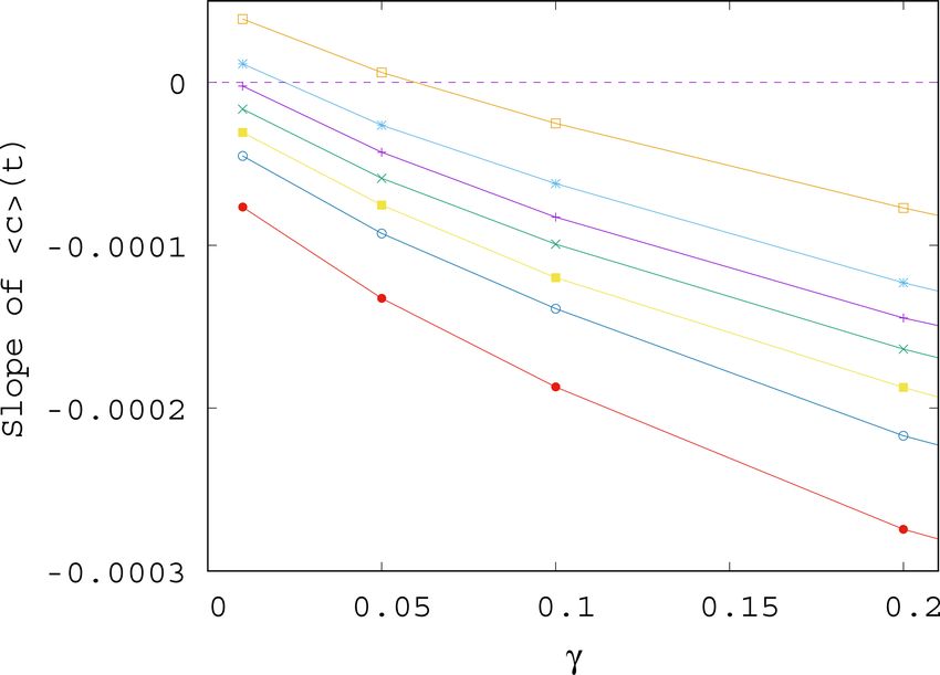
G. Károly et al.: Climate change in a conceptual atmosphere–phytoplankton model 607
Naively, one expects that an increased CO2 level (smaller in variable c, too. To explore this regime, we carried out a
F in Eq. 1) leads to a higher carrying capacity and concentra- sequence of numerical simulations of the full four-variable
tion of the phytoplankton, and a slower decrease of the tem- dynamics. The following parameters are kept fixed (as indi-
perature contrast, i.e., S (D) should increase (decrease) with cated in the previous section): r = 1, D0 = 2/7300, Fr = 9.5,
the enrichment parameter. However, only calculating the pre- A = 2, and ω = 2π/73. We vary α, β, and γ . Equations (1)
cise dependence can reveal whether these trends are impor- and (2) with (4), (8), and (9) are solved with the classi-
tant or hardly discernible. The linear coefficient slope S in cal fourth-order Runge–Kutta method with a fixed timestep
the phytoplankton concentration’s time dependence is found dt = 0.01 ≈ 1.37 × 10⁻⁴ years.
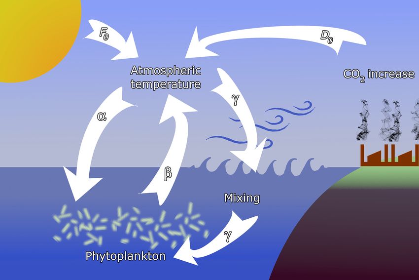
to be To start with, Fig. 2a shows a few individual concentration
D0 α realizations (colored lines) c(t) for a mixing parameter γ =
S= ≈ D0 α. (11) 0.1 (α = 0.05 and β = 0.1), along with the ensemble average
1 + βα
< c > (t) of 50 000 realizations initiated at t = −20 years
The approximate equality reflects that the product α · β is (purple line). Here and in what follows angled brackets
quadratically small, since both the enrichment parameter α will always denote averages taken with respect to our en-
and the extraction parameter β are small quantities. Hence semble at a given time instant, t. The individual cases are
the leading-order behavior in α is linear. This relation shows all rather different. For t < 0 there is no climate change, but
that for a positive (negative) coupling, α the phytoplankton nevertheless, the individual time series c(t) exhibits strong
concentration increases (decreases) proportionally with the variance, very similar to those observed for t > 0; i.e., they
enrichment parameter α and with the slope D0 of the anthro- are unable to properly reflect the ensemble and, in particular,
pogenic temperature contrast. the lack of climate change for t < 0. The ensemble average,
The linear coefficient in the temperature contrast is < c > (t), however, provides a plateau here up to t = 0, indi-
D0 cating clearly the stationarity of the climate and, therefore, of
D= ≈ D0 (1 − βα). (12) the biomass dynamics in this range. In Fig. 2b we display the
1 + βα
source of the time variability in the phytoplankton concentra-
The approximate equality provides, again, the leading-order tion, the total kinetic energy ẋ 2 + ẏ 2 + ż2 of the atmosphere at
behavior in α. The relation indicates that in the case of a pos- each time instant. The deviation of the individual ensemble
itive enrichment parameter α, the phytoplankton dynamics member time series from the average is represented here by
weakens the climate change, weakens the trend from D0 to D means of the standard deviation evaluated over the ensemble
in the temperature contrast, as expected. Quite surprisingly, (violet bars). The average kinetic energy, along with its en-
however, the effect is rather weak since α · β is quadratically semble variance, is also constant before the climate change
small. Relations (11) and (12) also suggest that the role of and starts an irregular time dependence right after t = 0. One
(a weak) extraction coupling is not essential; the leading be- can observe that the kinetic energy strongly influences the
havior in S is independent of β. Its effect is weak also in D. phytoplankton concentration (via the carrying capacity K in
This quantity coincides with the anthropogenic slope D0 for Eq. 9), but the concentration itself contributes to the CO2
β = 0 (as also follows from Eq. 4); it deviates from D0 very content and to the temperature contrast F – see Eq. (4) – forc-
little otherwise. ing the atmosphere (as will be demonstrated in Fig. 3). The
It is worth noting that relations (11) and (12) remain valid feedback of the atmosphere on phytoplankton is rather strong
for the time-averaged trends in the presence of a seasonal pe- in this setup with γ = 0.1, also expressed by the strong dif-
riodicity, as also shown in Sect. S1. Relations (11) and (12) ference between the green line (obtained for γ = 0) and the
are independent of initial conditions; they represent the snap- purple line in Fig. 2a illustrating that this coupling leads to
shot attractor of the problem projected on variable c. This an enormously enhanced biomass concentration.
attractor is fixed-point-like but changes in time (moves uni- It is visible in the inset to Fig. 2b that the ensemble av-
formly or with an oscillation superimposed when seasonality erage curve shows some change during the first 5 years (be-
is taken into account). There is, however, no internal vari- tween t = −20 and −15 years). This indicates (along with
ability in the concentration variable c, although an extended, several other simulations; not shown) that the convergence to
fractal snapshot attractor underlies the atmospheric variables the snapshot attractor takes about tc = 5 years. The numerical
exactly as in the model of Drótos et al. (2015), where phyto- data after t = −15 years thus represent parallel atmosphere–
plankton dynamics was not taken into account. phytoplankton realizations on the snapshot attractor of the
system.
4 Numerical results with mixing: trends in the fully The considerable deviation of the individual time series
coupled model from the ensemble average indicates that the formers are not
representing properly the mean climate state, as also pointed
In the interesting case of non-negligible mixing, no analytic out by Drótos et al. (2015). Therefore, from here on, we shall
result can be obtained. This implies a nontrivial biomass dy- concentrate on ensemble averages and consider the variance
namics for γ > 0, a dynamics exhibiting internal variability
https://doi.org/10.5194/esd-11-603-2020 Earth Syst. Dynam., 11, 603–615, 2020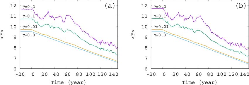
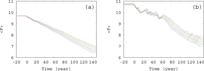
608                                          G. Károly et al.: Climate change in a conceptual atmosphere–phytoplankton model

Figure 2. Ensemble properties before (t < 0) and after (t > 0) the onset of climate change. (a) Phytoplankton concentration c as a function
of time for three random initial conditions in different colors for α = 0.05, β = 0.1, and γ = 0.1. The purple line is the ensemble average
< c > (t) for 50 000 trajectories started with random initial positions in the range x ∈ [−0.5, 3]; y, z ∈ [−2.5, 2.5]; and c ∈ [0.9, 1.1] at year
−20. The green line (close to c = 1) shows the expected phytoplankton concentration without any mixing (γ = 0) as predicted by Eq. (10).
(The increase for t > 0 is so weak that one hardly recognizes it on this graph.) (b) Time dependence of the ensemble average (dark violet
“+” marks) of the total atmospheric kinetic energy < ẋ 2 + ẏ 2 + ż2 > for the same ensemble as the one used for c in panel (a). Violet bars
indicate the standard deviation. The inset shows the blowup of the initial part of the average in panel (b).

Figure 3. Time dependence of the ensemble-averaged atmospheric forcing < F > (t) = F (< c > (t), t) in the case of γ = 0, 0.01, 0.1, and
0.2 for (a) α = 0.05 and (b) α = −0.05. The slope of the blue line for γ = 0 corresponds to D in Eq. (12).

in these as a measure of the internal variability (the size of             the fluctuations have longer timescale; hence the trends im-
the snapshot attractor in the chosen variable).                            posed by anthropogenic effects are less obvious, in particular,
   We carried out similar simulations with other extraction                on shorter timescales. A comparison of Fig. 3a and b belong-
parameter values from the range β ∈ [0.0, 0.5] and found                   ing to α = 0.05 and α = −0.05, respectively, indicates that a
that β does not have much effect on the average phyto-                     change in the sign of the enrichment parameter leads to only
plankton concentration, and the curves for various values of               minor differences in the general trends.
β are close to each other (see Fig. S1 in the Supplement                      Next, we study the dependence of the ensemble average
Sect. S2). In what follows, therefore, we stick to a single                of the phytoplankton concentration on the strength of mix-
value, β = 0.1.                                                            ing. We have seen in Fig. 2 that for γ = 0.1 strong deviations
   The time dependence of the typical (ensemble-averaged)                  appear from the trend, αD0 , occurring without mixing. The
temperature contrast < F > (t) forcing the atmospheric vari-               time dependence of < c > for mixing parameters on this or-
ables in Eq. (1) is shown in Fig. 3. The value of < F > (t)                der of magnitude, shown in Fig. S2, confirms the existence of
at each time instant is computed from Eqs. (4) and (8), with               large fluctuations. The time dependence of < c > for much
the average values < c > (ensemble average over 50 000 tra-                smaller values of γ are shown in Fig. 4. The linearly in-
jectories at that time instant) in place of c. The fluctuations            creasing trend in harmony with Eqs. (10) and (11) gradually
in the < F > (t) = F (< c > (t), t) curve of Fig. 3 follow the             disappears, and large-scale fluctuations are visible even for
fluctuations in the average phytoplankton concentration, but,              γ = 0.005.
for small values of γ , the linear decrease in F (t) is recov-                It seems that even a small coupling of the atmospheric
ered. In other words, for weak mixing (small values of γ )                 variables x, y, and z to the phytoplankton dynamics will re-
the trend in the forcing F (t) follows quite closely the direct            sult in large variations in < c > and in the suppression of the
anthropogenic trends. For strong mixing (γ ≥ 0.1), however,                anthropogenic trends on short terms. One can also conclude

Earth Syst. Dynam., 11, 603–615, 2020                                                           https://doi.org/10.5194/esd-11-603-2020
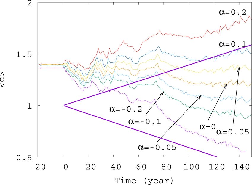
G. Károly et al.: Climate change in a conceptual atmosphere–phytoplankton model                                                     609

Figure 4. Ensemble-averaged phytoplankton concentration < c >          Figure 5. Average phytoplankton concentration < c > as a function
as a function of time for α = 0.05 for various values of γ (γ = 0,     of time for γ = 0.01 for various values of α (−0.2, −0.1, −0.05,
0.001, 0.002, 0.003, 0.004, and 0.005). The thick red line shows the   0.0, 0.05, 0.1, and 0.2). The thick purple lines show the expected
expected phytoplankton concentration in lack of mixing (γ = 0) as      phytoplankton concentration without mixing (γ = 0) as predicted
predicted by Eq. (11).                                                 by Eq. (11) for α = −0.2 (lower line) and α = 0.2 (upper line).

from these figures that a coupling with γ ≥ 0.002 should al-           hanced) climate change, this effect is quite small. The order
ready be considered strong in the atmosphere–ocean inter-              of magnitude of the effect of the phytoplankton concentra-
action, at least from the point of view of the phytoplankton           tion on < F > (t) can be assessed by observing in Fig. 5 that
dynamics.                                                              (< c > −1) falls between −0.5 and 1 at t = 150 years. Mul-
   Now we investigate the effect of the enrichment parame-             tiplied by our fixed β = 0.1, as Eq. (4) requires, one finds a
ter α on the phytoplankton concentration. We have seen in              range of 0.15, which is much smaller than the final value of
Fig. 4 that for small α = 0.05, the short-term trends are de-          F , about 7, at 150 years. This is comparable with the spread
stroyed for γ > 0.002. We see in Fig. 5 that with an increase          of the temperature contrast at the end of year 150 in Fig. 6a
in |α|, a trend might reappear at even higher values of the            and b. Note that these conclusions are drawn from the aver-
mixing parameter γ = 0.01. Indeed, for α between roughly               age temperature contrast. No trend can be extracted if instan-
−0.05 and 0.05, no trend is visible, and large scale fluctua-          taneous values of a single simulation are used instead of the
tions stemming from the internal variability in the dynamics           ensemble average, in the same spirit as in Fig. 2a.
rule the behavior of the average phytoplankton population.                Next, we study quantitatively how the trend observed in
For |α| ≥ 0.1, however, we see that trends emerge. There is            the ensemble average of the phytoplankton concentration
an increasing trend for positive and a decreasing trend for            changes with the parameters. To this end, we fit a straight line
negative α with a slope similar to the one given by the ana-           to the time dependence of the ensemble average < c > (t) of
lytic calculation valid for γ = 0.                                     the phytoplankton concentration for t > 0 for various values
   From the same set of α values used to construct Fig. 5, we          of parameters α and γ . The slope S(α, γ ) of the best-fit line
show the time dependence of the average forcing < F > (t)              in the presence of mixing gives information on the trend of
for an intermediate (γ = 0.01) and a large (γ = 0.1) mix-              the phytoplankton concentration, that is, on how quickly the
ing parameter in Fig. 6a and b, respectively. Interestingly, for       concentration changes with time on (ensemble) average. We
each value of α and γ , the < F > (t) graphs show a nearly             have also computed the standard deviations of this fit from
linear decay, the slope depending somewhat on α. It seems              the measured values to gain information on the fluctuations
that the direct anthropogenic component is dominant in the             appearing in individual members of the ensemble. We found
average forcing term, in particular for γ = 0.01, but this also        (not shown) that in case of a strong trend (slope of time de-
holds qualitatively for γ = 0.1 (see Fig. 6b). We thus con-            pendence far from zero) we find small fluctuations and vice
clude that a mixing parameter on the order of 0.1 is not yet           versa.
strong from the point of view of the forcing. This is in har-             In Fig. 7 we show the approximate slope S(α, γ ) of the
mony with the observation that the atmospheric kinetic en-             < c > (t) curves as a function of the mixing parameter γ .
ergy hardly depends on the mixing strength (see Fig. S3):              We see that the measured slopes, that is, the trends in the
the atmosphere is rather resistant to the feedback from the            time dependence, decrease with increasing values of γ . We
biomass.However, an increased (decreased) amount of phy-               also found that the fluctuations (not shown) are enhanced
toplankton present in the system results in an increased (de-          when γ increases. This implies that when mixing becomes
creased) temperature contrast, and hence, in a decreased (en-          stronger, the phytoplankton concentration is not only de-

https://doi.org/10.5194/esd-11-603-2020                                                    Earth Syst. Dynam., 11, 603–615, 2020
610                                        G. Károly et al.: Climate change in a conceptual atmosphere–phytoplankton model

Figure 6. Time dependence of the average forcing < F > (t) in the case of (a) γ = 0.01 and (b) γ = 0.1. The values of the enrichment
parameter from top to bottom are α = 0.2, 0.1, 0.05, 0, −0.05, −0.1, and −0.2.

                                                                      trends to be negative. It remains true, however, that the trend
                                                                      for a positive α is less negative than for a negative α. In other
                                                                      words, for sufficiently strong mixing, the phytoplankton con-
                                                                      centration always decreases with time due to climate change,
                                                                      and the sign of the enrichment parameter only influences the
                                                                      strength of decrease.
                                                                         If we plot the same data shown in Fig. 7 as a function of
                                                                      α instead of γ – see Fig. 8a – we see that the increase in the
                                                                      enrichment parameter increases the trend in the phytoplank-
                                                                      ton concentration. It is a surprising observation that even
                                                                      if the change in the mixing parameter changes the slopes
                                                                      essentially, their α dependence remains similarly linear as
                                                                      for γ = 0 given in Eq. (11). Plotting the slope −D(α, γ ) of
                                                                      the time-dependent, ensemble-averaged forcing < F > as a
Figure 7. Slope S of the ensemble average of the phytoplankton        function of α – see Fig. 8b – a very weak dependence is found
concentration, < c >, for t > 0 as γ is varied; data shown for var-   (note the vertical scale). On a closer look, the α dependence
ious values of α, from top to bottom, α = 0.2, 0.1, 0.05, 0, −0.05,
                                                                      is linear and increasing. This is in harmony with the expecta-
−0.1, and −0.2.
                                                                      tion that the CO2 extraction is weaker when the phytoplank-
                                                                      ton concentration is lower. With the exception of small γ
                                                                      values, the slopes are more negative than the direct anthro-
creasing for any α (the slope is negative) but also drops even        pogenic one, −D0 . It is a remarkable finding supported by
faster (the slope is decreasing). Note that the initial concen-       our results that a large mixing parameter enhances the speed
tration from which the decrease starts at t = 0 is higher for         of the climate change, irrespective of the sign of the enrich-
larger γ (stronger mixing); see Figs. 4 and S2. Concerning            ment parameter.
the fluctuations, we call the attention to the fact that in nearly       We see that the trends predicted by Eqs. (11) and (12) are
all figures exhibiting time dependence one can observe a de-          approached when γ is decreased. What is even more inter-
crease in the amplitude of variations for longer times, for           esting, the dependence of the trends on α remains the same
t > 100 years approximately. This appears to be a conse-              for any γ . In particular, we find a numerical fit of the slope S
quence of the decrease in the total atmospheric kinetic en-           of < c > (t) for β = 0.1 as
ergy with time, due to the overall decrease in the temperature
                                                                      S(α, γ ) = αD0 (1 + 3.8γ ) − 2D0 γ 0.75 .                   (13)
contrast in time, as Fig. S3 also illustrates. At a fixed mix-
ing parameter γ , the strength of mixing is proportional to           A similar expression is obtained from the slopes of the av-
the kinetic energy, which is thus decreasing in time. Since           eraged forcing < F > (t) that replaces D0 found in Eq. (12)
the carrying capacity is assumed to linearly depend on the            for γ = 0 by
kinetic energy (see Eq. 9), K also decreases in time. Thus,
                                                                      D(α, γ ) = D0 1 − αβ(1 + 3.8γ ) + 2βD0 γ 0.75 .

                                                                                                                             (14)
the phytoplankton concentration and its fluctuations are also
decreasing with time.                                                 It is surprising that the leading-order linear behavior in the
   It is worth also noting that even if for γ = 0 the trend in        enrichment parameter α found for S and D without any mix-
< c > would be increasing for positive enrichment parame-             ing remains valid for practically the entire γ range investi-
ters – see Eq. (11) – it is the increase in γ that converts all       gated; just the coefficients become γ dependent.

Earth Syst. Dynam., 11, 603–615, 2020                                                    https://doi.org/10.5194/esd-11-603-2020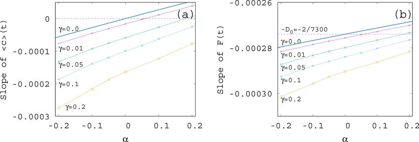
G. Károly et al.: Climate change in a conceptual atmosphere–phytoplankton model                                                       611

Figure 8. Slope (a) S of the ensemble-averaged phytoplankton concentration < c > (t) and (b) −D of the average forcing < F > for t > 0
as α is varied; data shown for various values of γ . The γ = 0 curve shows the α dependence of (a) S and (b) −D from Eqs. (11) and (12).
Dashed lines mark the slopes for α = 0 and γ = 0.

5   Snapshot attractors

The mathematical concepts underlying the ensemble view
are snapshot (Romeiras et al., 1990) or pullback (Ghil et al.,
2008) attractors. One might consider the ensemble of all per-
mitted climate realizations over all times as the pullback at-
tractor of the problem and the set of the permitted states of
the climate at a given time instant as the snapshot attractor
belonging to that time instant (their union over all time in-
stants is the pullback attractor). Both views express that the
climate system possesses a plethora of possibilities. In the
terminology of climate science, climate has a strong internal
variability (e.g., Stocker et al., 2013). The concept of snap-        Figure 9. The projection of the z = 0 and ż > 0 section of the snap-
shot or pullback attractors is nothing but a reformulation of         shot attractors on the x–y plane for β = 0.1, α = 0.05, and γ = 0.1.
this fact in dynamical terms.                                         The snapshot attractors at intervals of 10 years are shown with
   In numerical simulations, we consider the members of an            purple (t = −10 years), green (t = 0 years), cyan (t = 10 years),
ensemble simulation to describe parallel climate realizations         light orange (t = 20 years), yellow (t = 30 years), dark cyan (t =
only after the initial conditions are “forgotten”, and transient      40 years), dark red (t = 50 years), dark grey (t = 60 years), grey
dynamics disappears. Due to dissipation, this time is typi-           (t = 70 years), red (t = 80 years), light green (t = 90 years), blue
cally short compared to the time span of interest. Such an            (t = 100 years), pink (t = 110 years), light blue (t = 120 years),
                                                                      bright yellow (t = 130 years), black (t = 140 years), and dark or-
ensemble approach was shown to be the only method pro-
                                                                      ange (t = 150 years). They are generated by initiating 7 × 10⁷ ran-
viding reliable statistical predictions in systems with under-        dom initial conditions at year −20.
lying nonpredictable dynamics (since in this class the tradi-
tional approach based on a single time series is known to
provide seriously biased results). A number of papers illus-
trate these statements within the physics literature (see, e.g.,      instances separated by 10 years, clearly indicating that the
Romeiras et al., 1990; Lai, 1999; Serquina et al., 2008), as          attractor is changing in time. As the colors indicate, the pro-
well as in low-order climate models (Chekroun et al., 2011;           jection to the x–y plane of the z = 0 cross section of the snap-
Bódai et al., 2011; Bódai and Tél, 2012; Bódai et al., 2013;          shot attractor has a minimum size in years 60–80, after which
Drótos et al., 2015), in general circulation models (Haszpra          it increases again, and the maximum extension is reached by
and Herein, 2019; Kaszás et al., 2019; Pierini et al., 2018,          about year 150. Note that one cannot decide how much of
2016; Drótos et al., 2017; Herein et al., 2017; Bódai et al.,         the time dependence is a consequence of F0 (t) or the phy-
2020; Haszpra et al., 2020b, a), and also in experimental sit-        toplankton concentration. Due to the couplings between the
uations (Vincze, 2016; Vincze et al., 2017).                          biomass and the atmosphere, the direct anthropogenic effect
   For several parameter values, we also determined the snap-         cannot be separated from the effect of the biomass.
shot attractors of the coupled model. An example is given                 By investigating a projection of the snapshot attractor on
in Fig. 9 where we see the attractor on the z = 0 slice of            a plane containing concentration c as one of the axes, the
the atmospheric dynamics with the corresponding c values              influence of mixing on the internal variability within c can
not shown directly. Different colors indicate different time          be visualized. In Fig. 10, the z = 0 slice of the snapshot at-

https://doi.org/10.5194/esd-11-603-2020                                                    Earth Syst. Dynam., 11, 603–615, 2020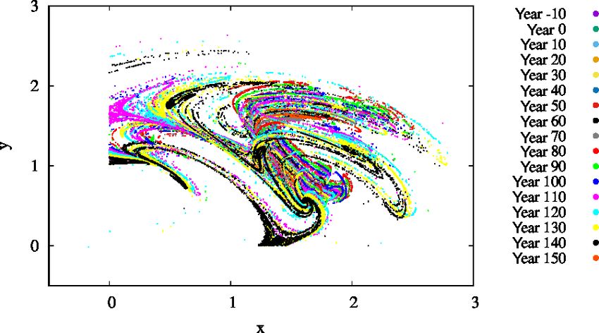
612                                        G. Károly et al.: Climate change in a conceptual atmosphere–phytoplankton model

                                                                      spheric forcing, modeling this way the extractions of CO2 by
                                                                      phytoplankton, but the same forcing is able to modify the
                                                                      carrying capacity via its coupling to the temperature con-
                                                                      trast characterized by the enrichment parameter. An addi-
                                                                      tional atmosphere–ocean coupling is also taken into account
                                                                      mimicking the enhancement of phytoplankton primary pro-
                                                                      duction via increased atmospheric activity, i.e., via turbulent
                                                                      mixing. Our intention has been to include leading-order ef-
                                                                      fects, and hence the coupling constants are chosen intention-
                                                                      ally to be small. Nevertheless, interesting consequences are
                                                                      found.
Figure 10. The projection of the z = 0 and ż > 0 section of the         By investigating the parameter dependence of the ensem-
snapshot attractors at year 150 on the x–c plane for β = 0.1 and      ble average of the atmospheric forcing and the phytoplankton
α = 0.05 and for γ = 0.0 (green), 0.003 (red), and 0.1 (blue).        content, we have shown that
                                                                        – even without mixing, the phytoplankton biomass in-
tractor of a given time instant is shown for three values of              teracts with the atmospheric forcing, and the coupling
γ , projected to the x–c plane; that is, the y values are not             between the phytoplankton concentration and the tem-
shown. We see that the extension of the snapshot attractor in             perature might weaken or strengthen the anthropogenic
the c direction is greatly affected by the strength of mixing:            warming trend; the increase or decrease in the phyto-
the c extension is zero for γ = 0 but increases rapidly for               plankton biomass depends on the sign of the enrichment
increasing γ . Parallel to this, the pattern becomes interwo-             parameter. In this regime, analytic results are available;
ven in the space of variables, suggesting that the c dynamics             see Eqs. (10), (11) and (12).
becomes more and more complex in time, too. It is the in-
                                                                        – increased mixing parameter enhances the total phyto-
creasing size and complexity of the snapshot attractor in the
                                                                          plankton population biomass. Stronger coupling may
c direction which is reflected in the increase in the strength
                                                                          enhance fluctuation to a degree that the anthropogenic
of fluctuations in Figs. 4 and S2.
                                                                          component practically disappears (Figs. 4 and S2).
   We also investigated the extremes of the snapshot attrac-
tors. That is, at a fixed time instant, we looked for those val-        – in contrast, mixing appears to depress the trend of the
ues of, e.g., x, for which only 10 % of values can be found               extraction of CO2 by phytoplankton and may force the
on the snapshot attractor below (lower extreme) or above                  phytoplankton population to globally decrease in time
(higher extreme) x. These values of x are shown in Fig. 11a               (see Fig. 7), although starting from a higher initial level.
as a function of time. The interval between these thresholds
is a measure of the size of the extension of the snapshot at-           – the coupling of mixing with phytoplankton biomass has
tractor at a given time instant. Clearly, this size undergoes             a much weaker effect on the atmospheric forcing (see
strong variations as a function of time. The same is shown                Fig. 6), as it is minimally expected from a coupled
in Fig. 11b for the time dependence of the c extension of the             atmosphere–phytoplankton model.
snapshot attractor: the upper (lower) curve shows the value
                                                                        – despite the strong modifications due to mixing, the de-
of c, above (below) which only 10 % of the values appear on
                                                                          pendence of trends on the strength of the coupling be-
the snapshot attractor. Again, we see considerable variations
                                                                          tween the phytoplankton concentration and the temper-
in time. It is interesting to note that, as these figures indicate,
                                                                          ature (the enrichment parameter) remains practically the
there is no unique trend in the size of the snapshot attractors,
                                                                          same as without mixing (see Fig. 8).
although trends can be seen in averages taken with respect
to the ensemble designating the attractor itself, like, e.g., in         We have obtained these results in a conceptual coupled
< c > or < F >.                                                       atmosphere–phytoplankton model which contains a tractable
                                                                      number of variables and parameters. To our knowledge, this
6   Conclusions                                                       is the first attempt to understand the general and robust fea-
                                                                      tures of the interplay between the atmosphere and the bio-
We have set up a conceptual coupled atmosphere–                       sphere in a climate change framework. One of our main re-
phytoplankton model by combining the Lorenz’84 general                sults is that an increase in the global temperature reduces
circulation model and the logistic equation under the con-            mixing intensity, which is the leading factor in decreasing the
dition of a climate change due to a linear decrease in the            total biomass of phytoplankton. Interestingly, this result is in
strength of direct anthropogenic forcing. The novel features          concordance with numerous studies applying Earth system
of the model are in the choice of the possible forms of cou-          models with vastly more detailed plankton models (Bopp et
plings. We allow for an influence of the biomass on the atmo-         al., 2013; Fu et al., 2016; Kwiatkowski et al., 2019), although

Earth Syst. Dynam., 11, 603–615, 2020                                                    https://doi.org/10.5194/esd-11-603-2020
G. Károly et al.: Climate change in a conceptual atmosphere–phytoplankton model 613
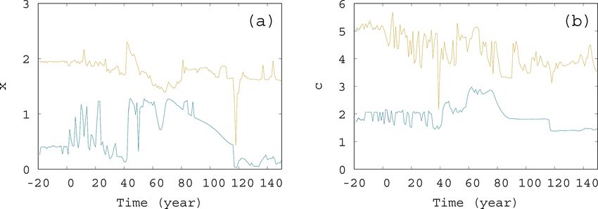
Figure 11. The extremes of the snapshot attractor for α = 0.05, β = 0.1, and γ = 0.1. Only 10 % of the points are found above (below) the
higher (lower) values for each time instant for (a) x and (b) c.
other works report different observations (Laufkötter et al., Supplement. The supplement related to this article is available
2015; Flombaum et al., 2020). online at: https://doi.org/10.5194/esd-11-603-2020-supplement.
As far as we know, our work is the first step in the direction
of studying the feedbacks between the atmosphere and the
biosphere by a simple conceptual model. Our conclusions are Author contributions. GK, IS, and TT worked out the outline of
robust in a mathematical sense, meaning that small changes the applied model, with a special contribution of IS to the biologi-
in our model (inclusion of noise, for example) will not al- cal background; GK and TT carried out the analytical calculations;
GK developed the simulation code; GK and RDP carried out the
ter our main findings, since snapshot attractors are robust.
simulations; all authors contributed to the preparation of the paper.
As long as the addition of other interactions only provide a
small perturbation, our conclusions remain valid. In general,
it is an open question in complex nonlinear systems whether Competing interests. The authors declare that they have no con-
neglected couplings to other subsystems and other simplifi- flict of interest.
cations could cause qualitative change in the dynamical be-
havior of a model. However, we see two important reasons
why we believe our model goes in the right direction. First, Acknowledgements. We are thankful for the useful comments
the trends we find in our model are in accordance with the from Tamás Bódai, Gábor Drótos, and Tímea Haszpra. This work
trends observed in the majority of complex models as men- was supported by the National Research, Development and Inno-
tioned above. Second, we believe that in our model the origin vation Office of Hungary under grant K-125171. István Scheuring
of trends is more transparent than in more complex models is supported by Hungary’s Economic Development and Innovation
where this origin can be hidden among the multitude of vari- Operative Program (GINOP 2.3.2-15-2016-00057). György Károly
ables, feedbacks, and interactions. Our model is a conceptual is supported by grant BME FIKP-VÍZ of EMMI.
model, and as such, both the biological and climate mod-
els are highly simplified. However, one can consider it as a
starting module of an extendable model system. On the one Financial support. This research has been supported by the NK-
FIH (grant no. K-125171), the GINOP (grant no. 2.3.2-15-2016-
hand, more trophical levels and inorganic resources can be
00057), and the EMMI (grant no. BME FIKP-VÍZ).
easily added to the biological side of our model; on the other
hand, simple ocean circulation models can extend the climate
side of our model in order to make a first step to build more Review statement. This paper was edited by Ben Kravitz and re-
complex coupled models (Daron and Stainforth, 2013). We viewed by two anonymous referees.
think that mutual interactions and iterations between concep-
tual models and detailed Earth system models (ESM) help
to reveal the distinction between relevant and less relevant
mechanisms and feedbacks behind climate change. We ex-
References
pect deeper insight into these feedbacks by studying concep-
tual models and ESMs parallelly in the future. Basu, S. and Mackey, K. R. M.: Phytoplankton as Key
Mediators of the iological Carbon Pump: Their Re-
sponses to a Changing Climate, Sustainability, 10, 869,
Code availability. The C language code applied during the simu- https://doi.org/10.3390/su10030869, 2018.
lations is included in the Supplement. Blunden, J. and Arndt, D. S.: State of the climate in 2012, B. Am.
Meteorol. Soc., 94, S1–S258, 2013.
https://doi.org/10.5194/esd-11-603-2020 Earth Syst. Dynam., 11, 603–615, 2020614 G. Károly et al.: Climate change in a conceptual atmosphere–phytoplankton model Bódai, T. and Tél, T.: Annual variability in a concep- Falkowski, P. G., Laws, E. A., Barber, R. T., and Murray, J. W.: Phy- tual climate model: Snapshot attractors, hysteresis in ex- toplankton and their role in primary, new, and export production, treme events, and climate sensitivity, Chaos, 22, 023110, in: Ocean Biogeochemistry. Global Change – The IGBP Series, https://doi.org/10.1063/1.3697984, 2012. edited by: Fasham, M. J. R., Springer, Berlin, Heidelberg, Ger- Bódai, T., Károlyi, Gy., and Tél, T.: A chaotically driven model many, 2003. climate: extreme events and snapshot attractors, Nonlin. Pro- Flombaum, P., Wang, W.-L., Primeau , F. W., and Martiny, A. cesses Geophys., 18, 573–580, https://doi.org/10.5194/npg-18- C.: Global picophytoplankton niche partitioning predicts overall 573-2011, 2011. positive response to ocean warming, Nat. Geosci., 13, 116–120, Bódai, T., Károlyi, Gy., and Tél, T.: Driving a concep- 2020. tual model climate by different processes: Snapshot at- Fu, W., Randerson, J. T., and Moore, J. K.: Climate change impacts tractors and extreme events, Phys. Rev. E, 87, 022822, on net primary production (NPP) and export production (EP) reg- https://doi.org/10.1103/PhysRevE.87.022822, 2013. ulated by increasing stratification and phytoplankton community Bódai, T., Drótos, G., Herein, M., Lunkeit, F., and Lucarini, V.: The structure in the CMIP5 models, Biogeosciences, 13, 5151–5170, Forced Response of the El Niño–Southern Oscillation–Indian https://doi.org/10.5194/bg-13-5151-2016, 2016. Monsoon Teleconnection in Ensembles of Earth System Models, Ghil, M.: Climate stability for a Sellers-type model, J. Atmos. Sci., J. Climate, 33, 2163–2182, 2020. 33, 3–20, 1976. Bopp, L., Resplandy, L., Orr, J. C., Doney, S. C., Dunne, J. P., Ghil, M., Chekroun, M. D., and Simonnet, E.: Climate dynamics Gehlen, M., Halloran, P., Heinze, C., Ilyina, T., Séférian, R., and fluid mechanics: Natural variability and related uncertainties, Tjiputra, J., and Vichi, M.: Multiple stressors of ocean ecosys- Phys. D, 237, 2111–2126, 2008. tems in the 21st century: projections with CMIP5 models, Guidi, L., Chaffron, S., Bittner, L., Eveillard, D., Larhlimi, A., Biogeosciences, 10, 6225–6245, https://doi.org/10.5194/bg-10- Roux, S., and Gorsky, G.: Plankton networks driving car- 6225-2013, 2013. bon export in the oligotrophic ocean, Nature, 532, 465–470, Chekroun, M. D., Simonnet, E., and Ghil, M.: Stochastic climate https://doi.org/10.1038/nature16942, 2016. dynamics: Random attractors and time-dependent invariant mea- Hader, D. P., Villafane, V. E., and Helbling, E. W.: Productivity of sures, Phys. D, 240, 1685–1700, 2011. aquatic +primary producers under global climate change, Pho- Chust, G., Allen, J. I., Bopp, L., Schrum, C., Holt, J., Tsiaras K., tochem. Photobiol. Sci., 13, 1370–1392, 2014. Zavatarelli, M., Chifflet, M., Cannaby, H., Dadou, I., Daewel, Haszpra, T. and Herein, M.: Ensemble-based analysis of the pollu- U., Wakelin, S. L., Machu, E., Pushpadas, D., Butenschon, M., tant spreading intensity induced by climate change, Sci. Rep., 9, Artioli, Y., Petihakis, G., Smith, C., Garçon, V., Goubanova, 3896, https://doi.org/10.1038/s41598-019-40451-7, 2019. K., Le Vu, B., Fach, B. A., Salihoglu, B., Clementi, E., and Haszpra, T., Herein, M., and Bódai, T.: Investigating ENSO Irigoien, X.: Biomass changes and trophic amplification of and its teleconnections under climate change in an ensemble plankton in a warmer ocean, Glob. Change Biol.,20 2124–2139, view – a new perspective, Earth Syst. Dynam., 11, 267–280, https://doi.org/10.1111/gcb.12562, 2014. https://doi.org/10.5194/esd-11-267-2020, 2020a. Daron, J. D. Stainforth, D. A.: On predicting climate un- Haszpra, T., Topál, D., and Herein, M.: On the Time Evolution of der climate change, Environ. Res. Lett., 8, 034021, the Arctic Oscillation and Related Wintertime Phenomena under https://doi.org/10.1088/1748-9326/8/3/034021, 2013. Different Forcing Scenarios in an Ensemble Approach, J. Cli- De La Rocha, C. L. and Passow, U.: The Biological Pump, Treatise mate, 33, 3107–3124, 2020b. on Geochemistry, 8, 93–122, https://doi.org/10.1016/B978-0-08- Herein, M., Drótos, G., Haszpra, T., Marfy, J., and Tél, 095975-7.00604-5, 2014. T.: The theory of parallel climate realizations as a new Drótos, G., Bódai, T., and Tél, T.: Probabilistic concepts in a chang- framework for teleconnection analysis, Sci. Rep., 7, 44529, ing climate: A snapshot attractor picture, J. Climate, 28, 3275– https://doi.org/10.1038/srep44529, 2017. 3288, 2015. Hutchins, D. A. and Fu, F.: Microorganisms and Drótos, G., Bódai, T., and Tél, T.: On the importance of the conver- ocean global change, Nat. Microbiol., 2, 17058, gence to climate attractors, Eur. Phys. J.-Spec. Top., 226, 2031– https://doi.org/10.1038/nmicrobiol.2017.58, 2017. 2038, 2017. Jäger, C. G., Diehl, S., and Emans, M.: Physical Determinants Estrada, M. and Berdalet, E.: Phytoplankton in a turbulent world, of Phytoplankton Production, Algal Stoichiometry, and Vertical Sci. Mar., 61, 125–140, 1997. Nutrient Fluxes, Am. Nat., 175, E91–E104, 2010. Falkowski, P. G.: Biogeochemistry of Primary Produc- Kaszás, B., Haszpra, T., and Herein, M.: The snowball tion in the Sea, Treatise on Geochemistry, 10, 163–187, Earth transition in a climate model with drifting parame- https://doi.org/10.1016/B978-0-08-095975-7.00805-6, 2014. ters: Splitting of the snapshot attractor, Chaos, 29, 113102, Falkowski, P. G., Barber, R. T., and Smetacek, V.: Biogeochemical https://doi.org/10.1063/1.5108837, 2019. controls and feedbacks on ocean primary production, Science, Kwiatkowski, L., Aumont, O., and Bopp L.: Consistent trophic 281, 200–206, 1998. amplification of marine biomass declines under climate change, Falkowski, P., Scholes, R. J., Boyle, E., Canadell, J., Canfield, Glob. Change Biol., 25, 218–229, 2019. D., Elser, J., Gruber, N., Hibbard, K., Hogberg, P., Linder, S., Lai, Y.-C.: Transient fractal behavior in snapshot attractors of driven Mackenzie, F. T., Moore III, B., Pedersen, T., Rosenthal, Y., chaotic systems, Phys. Rev. E, 60, 1558–1562, 1999. Seitzinger, S., Smetacek, V., and Steffen, W.: The global carbon Laufkötter, C., Vogt, M., Gruber, N., Aita-Noguchi, M., Aumont, cycle: A test of our knowledge of Earth as a system, Science, O., Bopp, L., Buitenhuis, E., Doney, S. C., Dunne, J., Hashioka, 290, 291–296, 2000. T., Hauck, J., Hirata, T., John, J., Le Quéré, C., Lima, I. D., Earth Syst. Dynam., 11, 603–615, 2020 https://doi.org/10.5194/esd-11-603-2020
You can also read