Examining the sensitivity of the terrestrial carbon cycle to the expression of El Niño
←
→
Page content transcription
If your browser does not render page correctly, please read the page content below
Biogeosciences, 18, 2181–2203, 2021
https://doi.org/10.5194/bg-18-2181-2021
© Author(s) 2021. This work is distributed under
the Creative Commons Attribution 4.0 License.

Examining the sensitivity of the terrestrial carbon cycle
to the expression of El Niño
Lina Teckentrup1,2 , Martin G. De Kauwe1,2,3 , Andrew J. Pitman1,2 , and Benjamin Smith4,5
1 ARC  Centre of Excellence for Climate Extremes, Sydney, NSW, Australia
2 Climate Change Research Centre, University of New South Wales, Sydney, NSW, Australia
3 Evolution & Ecology Research Centre, University of New South Wales, Sydney, NSW 2052, Australia
4 Hawkesbury Institute for the Environment, Western Sydney University, Penrith, NSW, Australia
5 Department of Physical Geography and Ecosystem Science, Lund University, Lund, Sweden

Correspondence: Lina Teckentrup (l.teckentrup@unsw.edu.au)

Received: 3 August 2020 – Discussion started: 20 August 2020
Revised: 18 December 2020 – Accepted: 24 January 2021 – Published: 25 March 2021

Abstract. The El Niño--Southern Oscillation (ENSO) influ-         1   Introduction
ences the global climate and the variability in the terrestrial
carbon cycle on interannual timescales. Two different expres-
sions of El Niño have recently been identified: (i) central Pa-   The terrestrial carbon cycle varies markedly on interannual
cific (CP) and (ii) eastern Pacific (EP). Both types of El Niño   timescales and is significantly influenced by the El Niño–
are characterised by above-average sea surface temperature        Southern Oscillation (ENSO) at global scales. Around 20%
anomalies at the respective locations. Studies exploring the      of the vegetated land shows a significant negative correlation
impact of these expressions of El Niño on the carbon cycle        with the ENSO cycles, predominantly in the tropics and in
have identified changes in the amplitude of the concentra-        arid areas. Around 12% of vegetated land is positively corre-
tion of interannual atmospheric carbon dioxide (CO2 ) vari-       lated with ENSO cycles, with this correlation dominated by
ability following increased tropical near-surface air temper-     arid areas (Zhang et al., 2019). In general, ENSO is positively
ature and decreased precipitation. We employ the dynamic          skewed such that El Niño events have a stronger effect on
global vegetation model LPJ-GUESS (Lund–Potsdam–Jena              the terrestrial carbon cycle than La Niña events (e.g. Haverd
General Ecosystem Simulator) within a synthetic experimen-        et al., 2017; Ahlström et al., 2015). During El Niño events,
tal framework to examine the sensitivity and potential long-      terrestrial ecosystems typically act as a carbon source, while
term impacts of these two expressions of El Niño on the ter-      during La Niña events carbon uptake is enhanced, particu-
restrial carbon cycle. We manipulated the occurrence of CP        larly in semi-arid ecosystems (e.g. Ahlström et al., 2015).
and EP events in two climate reanalysis datasets during the       Multiple studies have examined the effect of El Niño on
latter half of the 20th and early 21st century by replacing all   the terrestrial carbon cycle using observations and ecosys-
EP with CP and separately all CP with EP El Niño events.          tem models (e.g. Bastos et al., 2018; Rödenbeck et al., 2018;
We found that the different expressions of El Niño affect in-     Zhang et al., 2019; Fang et al., 2017). Given the influence of
terannual variability in the terrestrial carbon cycle. However,   ENSO on the interannual variability (IAV) of the terrestrial
the effect on longer timescales was small for both climate        carbon cycle, representing ENSO and associated teleconnec-
reanalysis datasets. We conclude that capturing any future        tions is important in coupled Earth system modelling (e.g.
trends in the relative frequency of CP and EP El Niño events      Kim et al., 2016; Qian et al., 2008).
may not be critical for robust simulations of the terrestrial        Each El Niño event varies in terms of the pattern and in-
carbon cycle.                                                     tensity of sea surface temperature anomalies. Recent analy-
                                                                  ses have highlighted two distinct expressions or flavours of
                                                                  El Niño: the (i) central Pacific (CP) and (ii) eastern Pacific
                                                                  (EP) El Niño (Donguy and Dessier, 1983; Ashok et al., 2007;

Published by Copernicus Publications on behalf of the European Geosciences Union.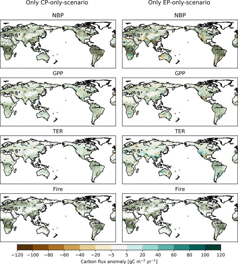
2182                                           L. Teckentrup et al.: Examining the sensitivity of the terrestrial carbon cycle

Weng et al., 2007). Both expressions of El Niño are char-           which currently struggle to correctly resolve El Niño–La
acterised by above-average sea surface temperature anoma-           Niña cycles with the correct persistence and teleconnections
lies at their respective locations. Depending on the location       (Bellenger et al., 2014). If the expression of El Niño, as dis-
of the sea surface temperature anomalies, these different ex-       tinct from El Niño in general, is shown to affect IAV as well
pressions of El Niño are associated with different impacts          as the longer-timescale terrestrial carbon balance, this would
on the Walker circulation, different teleconnection patterns,       place a significantly higher demand on climate models to ac-
and therefore different regional-scale rainfall and tempera-        curately reproduce both the persistence and teleconnections
ture anomalies (e.g. Taschetto and England, 2009; Ashok             of the El Niño–La Niña cycles, and the relative frequency
et al., 2009; Weng et al., 2007; Ashok et al., 2007). For ex-       in the future of CP and EP El Niño events. This could sig-
ample, Taschetto and England (2009) found that maximum              nificantly constrain our capacity to predict the future of the
rainfall decreases associated with EP El Niño events tend to        terrestrial carbon cycle.
occur over northeastern and southeastern Australia, while CP           To explore whether the expression of El Niño affects
El Niño events are associated with a negative precipitation         the global and regional terrestrial carbon cycle on multi-
response in northwestern and northern Australia. Further, the       decadal timescales, we use a dynamic global vegetation
timing of the maximum precipitation anomalies varied with           model (DGVM) forced by the climate data obtained from
the expression of El Niño. Given the different expressions of       two reanalysis datasets. We generate two synthetic forcing
El Niño, and the consequential differences in regional rain-        datasets: one where, starting 1968, all El Niño events are a
fall and temperature, a different ecosystem response might          CP type and one where all El Niño events are an EP type.
be expected between CP and EP El Niño events. A shift in El         We then use our DGVM experiments to examine the impact
Niño patterns could change cumulative net biome production          of the expression of El Niño on the global terrestrial carbon
(NBP), which may alter competitive patterns of plant func-          cycle.
tional types, both of which may influence the carbon stored in
vegetation and soil (e.g. Park et al., 2020). Similarly, interan-
nual variability in precipitation patterns induced by different
types of El Niño might result in a shift in vegetation distri-      2     Methods
butions, particular at climatic transition zones or in water-
limited environments, for example semi-arid areas and sa-           2.1    Model
vanna ecosystems (cf. Scheiter and Higgins, 2009; Whitley
et al., 2017). Recent studies have found that, depending on         LPJ-GUESS (Lund–Potsdam–Jena General Ecosystem Sim-
the expression of El Niño, different time lags, amplitudes and      ulator; Smith et al., 2001, 2014) is a DGVM extensively
duration in the carbon cycle anomalies occur (Wang et al.,          used for climate–carbon studies (Smith et al., 2014; Sitch
2018; Chylek et al., 2018). Wang et al. (2018) and Chylek           et al., 2003). LPJ-GUESS is used as the land surface scheme
et al. (2018) link the effects of different expressions of El       in the global Earth system model EC-Earth3 (Weiss et al.,
Niño on the terrestrial carbon cycle to variability at interan-     2014; Alessandri et al., 2017) and in the regional Earth sys-
nual timescales, but the impact on longer timescales is not         tem model RCA-GUESS (Wramneby et al., 2010; Zhang
well understood.                                                    et al., 2014). LPJ-GUESS dynamically simulates the ex-
   While it is clear that El Niño has an impact on the ter-         change of water, carbon and nitrogen through the soil–
restrial carbon cycle, analyses that have demonstrated this         plant–atmosphere continuum (Smith et al., 2014), resolving
mostly have not attempted to separate El Niño into CP and           the vegetation’s resource competition for light and space.
EP types. Understanding the sensitivity of the terrestrial car-     LPJ-GUESS groups the vegetation into 12 plant functional
bon cycle to these distinct El Niño expressions is a key            types (PFTs), simulating differences in growth form (grasses,
knowledge gap, specifically because there is evidence that          broadleaved trees or deciduous trees), photosynthetic path-
the relative frequency of CP and EP El Niños may be chang-          way (C3 or C4 ), phenology (evergreen, summer green or rain
ing. There is emerging evidence that in the late 20th and early     green), tree allometry and life history strategy, fire sensitiv-
21st century the occurrence of CP El Niño events increased          ity, and bioclimatic limits for establishment and survival.
in frequency (Yu and Kim, 2013), and some studies using cli-           We use LPJ-GUESS version 4.0.1 in “cohort mode”,
mate projections suggest that this trend will continue as the       where woody plants of the same size and age co-occurring
atmospheric carbon dioxide (CO2 ) concentration increases           in a local neighbourhood or “patch” are represented by a sin-
(e.g. Yeh et al., 2009). Despite recent research finding that the   gle average individual. Each PFT is represented by multiple
expression of El Niño is important at interannual timescales        average individuals, and one PFT cohort is defined as the av-
(Wang et al., 2018; Chylek et al., 2018; Pan et al., 2018), it is   erage of several individuals. Assuming that all individuals
not known how and where the recent trend towards more CP            of the same age in a particular patch have the same structure,
El Niño events would impact the terrestrial carbon cycle.           then several cohorts form a single patch. Establishment, mor-
   This re-focussing towards the specific expression of El          tality and disturbance are stochastic processes. Fire is sim-
Niño is potentially problematic for global climate models,          ulated annually (stochastically) based on temperature, fuel

Biogeosciences, 18, 2181–2203, 2021                                                    https://doi.org/10.5194/bg-18-2181-2021
L. Teckentrup et al.: Examining the sensitivity of the terrestrial carbon cycle                                            2183

availability and the moisture content of upper soil layer as a    out of these four indices agree on the same El Niño type. The
proxy for litter moisture content (Thonicke et al., 2001).        remaining events are defined as mixed events (“MIX”; see
                                                                  Appendix Table A1; compare Table 1 in Yu and Kim, 2013).
2.2   Forcing                                                        Note that our approach defines the 1968–1969 El Niño
                                                                  event as the first CP El Niño event and consequently the first
LPJ-GUESS requires soil texture (Zobler, 1986; Sitch et al.,      year of our experiment set-up. Given the climate forcing is
2003), daily temperature, precipitation, incoming shortwave       limited to 1901–2015, we exclude the 2015–2016 El Niño
radiation and the annual mean atmospheric carbon dioxide          event and choose the ENSO-neutral year 2013 as the final
(CO2 ) concentration. The atmospheric CO2 concentration,          year. We analyse the effect that a climate with only CP El
varying annually, was compiled from atmospheric measure-          Niño or only EP El Niño events might have on terrestrial
ments (McGuire et al., 2001; Smith et al., 2014). We used         vegetation after 45 years by comparing the final year of the
the CRUNCEP V7 dataset (Viovy, 2018) as the meteorolog-           two different scenarios to that of the control run (where both
ical forcing input for LPJ-GUESS. CRUNCEP is based on             expressions of El Niño occur).
a merged observed monthly climatology product of the Cli-
mate Research Unit (CRU) and the high-temporal-resolution         2.5   Experiment design
reanalysis by the National Centers for Environmental Predic-
tion (NCEP). The spatial resolution is 0.5◦ and the temporal      In the control run, we ran LPJ-GUESS with the original
resolution is 6 h for the time period 1901–2016. From the         CRUNCEP forcing for the period 1901–2015. For the exper-
CRUNCEP data, we calculated daily averages of the temper-         iment simulations, we created two climate forcing datasets
ature and incoming shortwave radiation and daily sums of          containing either only CP or only EP El Niño events starting
the precipitation as inputs for LPJ-GUESS.                        from 1968, hereafter referred to as CP-only and EP-only. To
   To explore the sensitivity of our results to differences       do this, we replaced climate anomalies associated with CP El
in the meteorological forcing, we repeated our experiments        Niño events with those of EP El Niño events and vice versa
using the Global Soil Wetness Project Phase 3 (GSWP3)             for the three climate variables temperature, precipitation and
dataset (Kim, 2017). GSWP3 is based on the 20th Century           incoming shortwave radiation. In this study, we focussed our
Reanalysis (20CR; Compo et al., 2011), which is dynami-           analysis on the tropics (23◦ S–23◦ N) and Australia in addi-
cally downscaled from a global 2◦ resolution with a 3 h tem-      tion to a global analysis.
poral resolution into a T248 (∼ 0.5◦ ) grid using a spectral         To generate the synthetic CP and EP forcing datasets,
nudging technique (Yoshimura and Kanamitsu, 2008) in a            we take the reanalysis forcing (displayed schematically in
global spectral model. Since GSWP3 only covers the time           Fig. 1a) and first calculate eight 30-year averages that are
period of 1901–2010, we choose the CRUNCEP-based simu-            used as base periods (see Fig. 1b) for every grid point based
lations for the main analysis and use the GSWP3-based sim-        on the original climate forcing (see Fig. 1a). Each base pe-
ulations to determine if the meteorological forcing leads to      riod is used to calculate the anomalies for successive 5-year
major differences in our results.                                 periods; i.e. we compare the years from 1966–1970 to the
                                                                  average over 1951–1980, the years from 1971–1975 to the
2.3   Model set-up
                                                                  average over 1956–1985 and so on. The last 15 years (2001–
LPJ-GUESS was spun up for 500 years using the first               2015) are compared to the average over 1986–2015 (see
30 years of the climate forcing (1901–1930) to allow the car-     Fig. 1c; compare calculation of ONI in Lindsey, 2013). We
bon pools to reach equilibrium. During the spin-up, tempera-      subtract these base periods from the original forcing for each
ture is detrended and the climate forcing is cycled repeatedly    pixel and identify anomalies associated with the type of El
with a constant atmospheric CO2 concentration of 296 ppm.         Niño according to Table A1 (see Fig. 1d). We used the ONI
After the spin-up, the simulation continues with the historical   to define the start, end and strength of the individual El Niño
climate and transient atmospheric CO2 forcing (e.g. Smith         events and resampled the climate anomalies based on the
et al., 2014). For this study, we allow for fire and stochas-     ONI. We replaced anomalies in the climate forcing associ-
tic disturbance. We do not account for recent anthropogenic       ated with El Niño events according to the best fit in duration
changes in global land use cover.                                 and amplitude in ONI, i.e. events that start and end at a sim-
                                                                  ilar time in the year and have a similar timing and magni-
2.4   Identification of El Niño events                            tude of the peak in ONI. For the replacement of the climate
                                                                  anomalies, we defined the start of an El Niño event as the
We base the identification of El Niño events on a study by Yu     second month of the first ONI season and the end as the sec-
and Kim (2013). They first classified El Niño events based        ond month of the last ONI season for each El Niño event
on the Oceanic Niño Index (ONI), which comprises both CP          (see Fig. 1e and f). For example, the El Niño event from
and EP El Niño events. Based on four indices, they then fur-      1968–1969 started in the ONI season September–October–
ther differentiate between CP and EP El Niño events. For          November and ended in April–May–June, so the first month
this study, we define a CP or EP El Niño event when three         of the 1968–1969 El Niño event is October in 1968 and the

https://doi.org/10.5194/bg-18-2181-2021                                                  Biogeosciences, 18, 2181–2203, 2021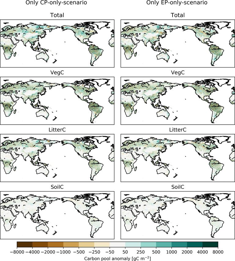
2184 L. Teckentrup et al.: Examining the sensitivity of the terrestrial carbon cycle
last month is March in 1969. Finally, we added the new TER varied by smaller amounts for all regions (see Fig. 3b, e,
anomalies and the original base periods to create the manip- h). Carbon fire emissions responded weakly to the expression
ulated climate forcing. of the El Niño (see Fig. 3c, f, i). All fluxes show higher vari-
This approach only isolates the effect of different expres- ability through to the end of the 20th century compared to the
sions of El Niño to a limited extent since the calculated early 21st century. The lower variability in the 21st century
anomalies can also be influenced by other climate modes of coincides with a period of a positive phase in the Interdecadal
variability. For example in Australia and Indonesia, differ- Pacific Oscillation.
ent expressions of El Niño and different phases of the Indian However, the IAV does not lead to sustained trends in the
Ocean Dipole can combine to drive the fire season (e.g. Pan ecosystem fluxes. The spatial distribution of the flux anoma-
et al., 2018). Given we create two synthetic forcings with 15 lies in the final year of the experiment (2013) displays spa-
CP (nine events replaced) and 15 EP (eight events replaced) tial variability rather than systematic patterns, implying that
El Niño events, we assume that the emerging signal in the the imposed changes also did not lead to long-term shifts
model results will be representative of the effect of different in ecosystem processes at regional scales (see Appendix
expressions of El Niño on the carbon balance. Fig. B1).
We use an identical approach for the GSWP3 dataset. The Figure 3 also shows the accumulated change in fluxes be-
only difference is the shorter length of the time period cov- tween 1968 and 2013. The cumulative sums of the absolute
ered: GSWP3 ends in 2010; hence the last base period calcu- differences for fire carbon emissions are between −0.8 and
lated is the average over 1981–2010 instead of 1985–2015 as 0.3 PgC for the CP- and the EP-only scenario, respectively
for CRUNCEP. (see Fig. 3c). Over the 45 years, the accumulated GPP leads
We processed the data with netCDF Operators (ver- to a difference of 60.2 and 35.8 PgC for the CP- and the EP-
sion 4.7.7, http://nco.sf.net, last access: 27 October 2020) and only scenario, respectively, and this is largely balanced by
Climate Data Operators (version 1.9.5, http://mpimet.mpg. the accumulated TER, 50.3 and 26.6 PgC for the CP- and
de/cdo, last access: 27 October 2020). The data analysis is the EP-only scenario, respectively (see Fig. 3a, b). For NBP,
conducted with Python version 3. GPP and TER, a CP-only scenario leads to stronger increases
compared to an EP-only scenario both globally and for trop-
ical regions (see Figs. 2g, h, 3a, b, d, e). In Australia, the cu-
3 Results mulative sums of GPP and TER anomalies in a CP-only sce-
nario start to converge with the cumulative anomalies in an
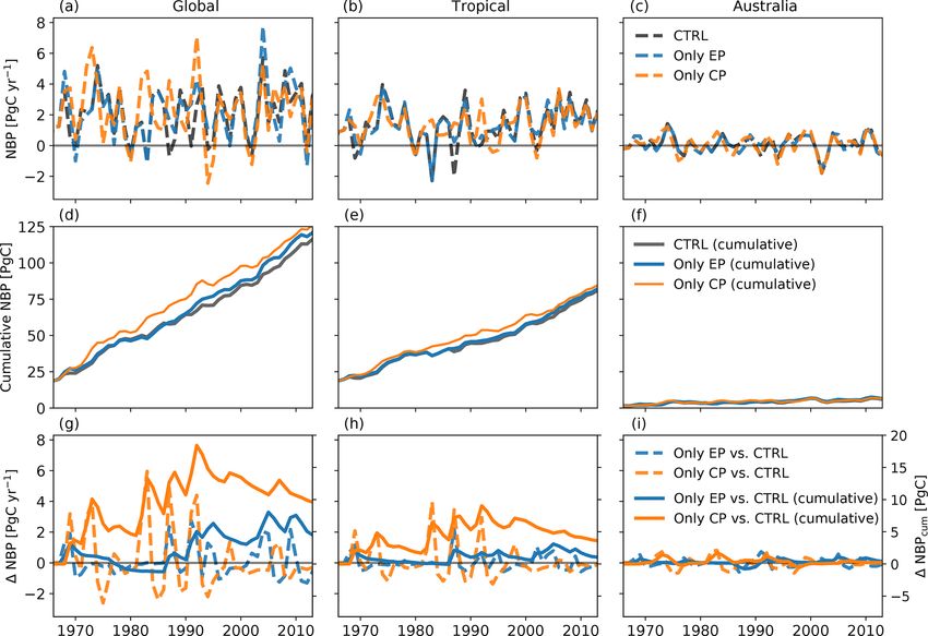
Figure 2 shows the effect of different expressions of El Niño EP-only scenario in 2005 for GPP and TER so that they reach
on the NBP. The upper three panels (Fig. 2a, b, c) display to- similar values in 2013 (CP-only scenario: 7.4 PgC for GPP
tal global NBP as well as tropical and Australian NBP for the and 6.2 PgC for TER; EP-only scenario: 7.3 PgC for GPP
control run and for the two experiments. All three runs have and 5.9 PgC for TER; see Fig. 3g, h). The cumulative car-
a similar magnitude in the IAV of NBP. Both the CP- and EP- bon lost through fires declines in a CP-only scenario globally
only scenarios can increase or dampen the peaks in NBP for and in the tropical regions and is close to zero for Australia
the different regions. For all three regions, NBP accumulates (see Fig. 3c, f, i). In contrast to the absolute differences in
to around 120 PgC globally, 80 PgC for the tropics and 6 PgC the fluxes in the year 2013 (see above), cumulative GPP and
for Australia (see Fig. 2d–f). Overall, cycling of carbon (IAV TER show a clear(er) pattern with increases for both fluxes
of NBP) through the terrestrial biosphere was most marked in southern South America and over Australia (see Appendix
in CP years relative to EP years (see Fig. 2g, h and i). The Fig. B3). The accumulated increases in GPP however are bal-
magnitude in the difference of annual NBP in the CP- and anced by increases in TER so that cumulative NBP shows
EP-only scenarios compared to the control run is compara- strong spatial variability similar to the fluxes in Appendix
ble to the total IAV of NBP (compare Fig. 2a, b, c). Overall, Fig. B1.
global changes in NBP accumulate to 9.6 and 4.5 PgC for the At the global scale, the CP-only simulations led to an in-
CP- and the EP-only scenario, respectively (see Fig. 2g). crease in the total land carbon storage (see Fig. 4a). Between
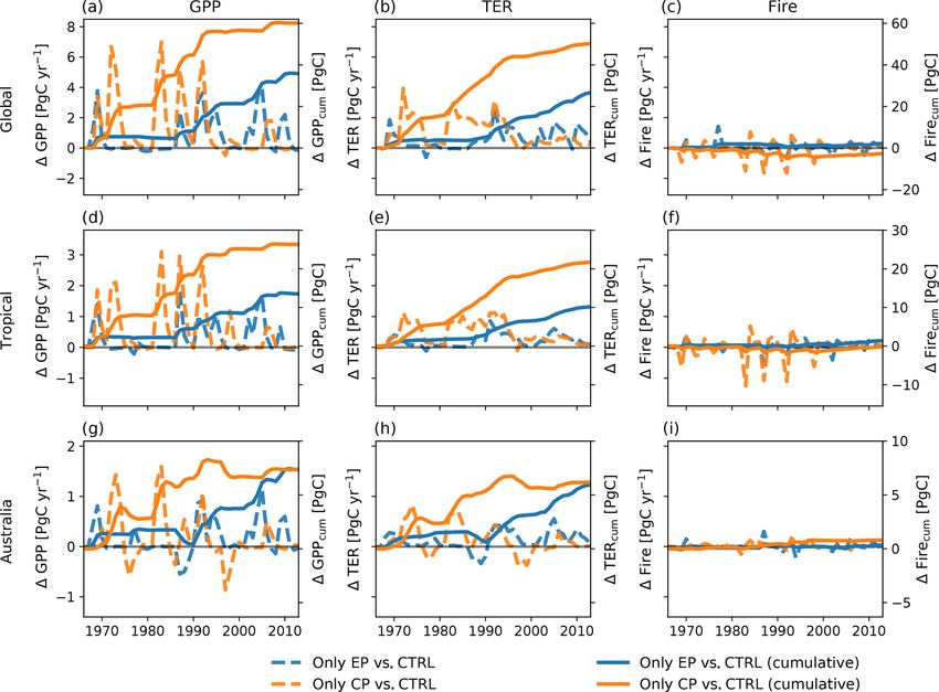
Figure 3 breaks down the NBP response to the three terres- 1968 and 2013, the total carbon stored increased by 9.6 PgC
trial ecosystem fluxes gross primary production (GPP), ter- compared to the control run (see Fig. 4a, “Total”; i.e. the
restrial ecosystem respiration (TER, the sum of autotrophic sum of carbon stored vegetation, litter and soil). The EP-
and heterotrophic respiration) and fire emissions. Prior to only simulations led to a gain of ∼ 4.5 PgC relative to the
1997, individual CP events led to large IAV, with increases control run (see Fig. 4d). Figure 4 also shows the breakdown
in global GPP in some years of up to 7 PgC yr−1 and of the change in carbon storage between the vegetation, litter
reductions in some years of around −0.5 PgC yr−1 (see and soil pools. In the CP-only simulation, the total change is
Fig. 3a). Changes in tropical GPP were mostly positive (up to dominated by an increase in vegetation carbon of ∼ 5.5 PgC
3.1 PgC yr−1 ; see Fig. 3b). By contrast, in drier regions, for originating from cumulative changes in GPP outbalancing
example in Australia, the year-to-year variability ranged be- those of TER. By contrast, in the EP-only simulations, any
tween −0.9 and 1.6 PgC yr−1 (see Fig. 3g). By comparison, short-term increases in vegetation biomass are balanced by
Biogeosciences, 18, 2181–2203, 2021 https://doi.org/10.5194/bg-18-2181-2021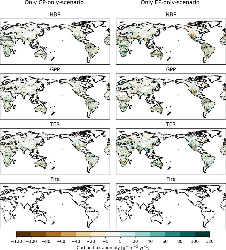
L. Teckentrup et al.: Examining the sensitivity of the terrestrial carbon cycle                                                    2185

Figure 1. Schematic figure for the generation of the synthetic CP and EP forcing datasets (see text for details).

increased respiration, tissue turnover and mortality, leading             Ashok et al., 2009). While the impact of more extreme (EP)
to a negligible change in ecosystem carbon storage. In both               El Niño events has been examined (e.g. Kim et al., 2017),
the CP- and EP-only scenario, the total differences in terres-            there are few studies exploring the impact of different ex-
trial carbon pools are largely the result of the responses of             pressions of El Niño on the terrestrial carbon cycle. Previous
tropical ecosystems. Similar to the carbon fluxes, no clear               work has focussed on short timescales and explored time lag
patterns in the spatial distribution of the carbon pool anoma-            effects on the carbon growth rate (Chylek et al., 2018), single
lies emerge (see Appendix Fig. B4).                                       regions and/or single events (Amazonia, Li et al., 2011; In-
                                                                          donesia, Pan et al., 2018), or the composite anomalies in the
                                                                          carbon fluxes (Wang et al., 2018) in a larger spatial context.
4   Discussion                                                            In effect, the response of ecosystems to different expressions
                                                                          of El Niño on longer timescales is not well understood.
The El Niño–Southern Oscillation strongly influences global                  In this study we show that, in line with previous studies
and regional climate and has the potential to modify the re-              (e.g. Wang et al., 2018; Chylek et al., 2018), climate anoma-
gional and global carbon balance. Here, we examine whether                lies associated with different expressions of El Niño have a
two expressions of El Niño (CP and EP), as distinct from the              strong impact on the IAV of ecosystem carbon fluxes. The
El Niño phenomenon itself, modify the regional and global                 El Niño-associated climate anomalies in our experiments do
carbon balance. This is timely: EP El Niño events might be-               not show a consistent pattern but rather display high tempo-
come more extreme in the future (e.g. Wang et al., 2019; Cai              ral variability between individual El Niño events (see Ap-
et al., 2018), and the occurrence of CP El Niño events seems              pendix Fig. B5). Wang et al. (2018) showed that between
to have increased over the latter half of the 21st century                El Niño events the atmospheric CO2 growth rate varied by
and may increase further in the future (e.g. Yeh et al., 2009;            4 PgC yr−1 at the peak for EP events and ∼ 2 PgC yr−1 for

https://doi.org/10.5194/bg-18-2181-2021                                                            Biogeosciences, 18, 2181–2203, 2021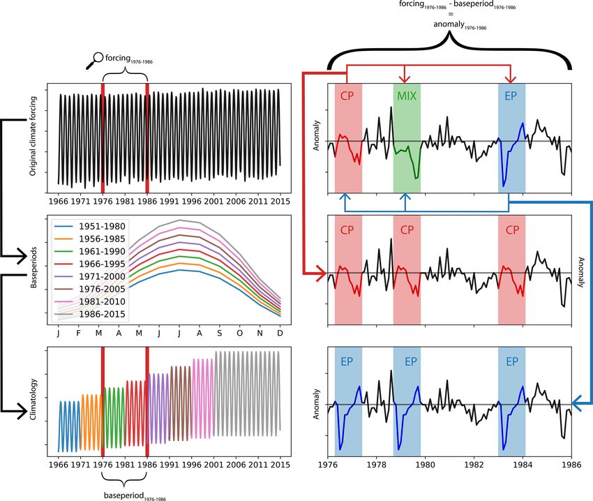
2186                                            L. Teckentrup et al.: Examining the sensitivity of the terrestrial carbon cycle

Figure 2. Total net biome production (NBP) (a–c), cumulative NBP (d–f), and absolute difference and cumulative sums of the difference
between CP-only scenario and control climate and EP-only scenario and control climate (g–i).

CP events. Consequently, the ecosystem fluxes vary strongly          the carbon balance in drier ecosystems and/or water-limited
in their response to different expressions of El Niño for indi-      agricultural regions. Interconnections between the terrestrial
vidual years.                                                        carbon cycle and ENSO have been widely explored (e.g.
   Despite the large resulting IAV in ecosystem carbon               Zhang et al., 2019; Rödenbeck et al., 2018; Chylek et al.,
fluxes, the changes in GPP show a clear cumulative global in-        2018). While we also find key NBP variability on annual-to-
crease of about 60 PgC (CP-only scenario) and 36 PgC (EP-            decadal timescales (see Fig. 2), particularly in CP years (ac-
only scenario) over the 45 years simulated (see Fig. 3 a, d,         cumulated NBP = 9.6 PgC), we did not find that this shorter
g). In both scenarios, additional photosynthetic carbon up-          timescale variability translated into sustained trends (1968–
take was mostly balanced by terrestrial ecosystem respiration        2013) in ecosystem fluxes, or shifts in vegetation distribu-
(50 PgC for CP-only scenario, 27 PgC for EP-only scenario;           tions (see Fig. 3).
see Fig. 3 b, e, h). This, and the strong interannual variability,
leads to small net changes in cumulative NBP over 45 years.          4.1   Future directions
The strong IAV in NBP therefore only results in a minor
change in the total carbon storage simulated over 45 years,
                                                                     In our study we used a dynamic global vegetation model
with 9.6 PgC more in a CP-only scenario and ∼ 4.5 PgC more
                                                                     to examine the sensitivity of the terrestrial carbon cycle to
in the EP-only scenario (see Fig. 4 a, d).
                                                                     changes in El Niño patterns. In response to climate, DGVMs
   Overall, the high spatial and temporal variability in the
                                                                     predict global vegetation distributions based on plant phys-
changes suggest that the effect of different expressions of
                                                                     iology, competition, demography and vegetation structure
El Niño on the terrestrial carbon cycle is important for pre-
                                                                     (Sitch et al., 2003; Woodward and Lomas, 2004). In par-
dicting responses on interannual timescales (e.g. the atmo-
                                                                     ticular, these models also consider how fire dynamics and
spheric CO2 growth rate) but is unlikely to affect the terres-
                                                                     vegetation composition may respond to a shift in climate.
trial carbon balance on longer timescales. Our model results
                                                                     In the past DGVMs have been widely used to examine how
imply that the anomaly patterns in the El Niño expression on
                                                                     vegetation distributions may change in response to climate
climate forcing were too variable (and short-lived) to result
                                                                     (Hickler et al., 2012; Martens et al., 2020) and fire (Kel-
in systematic shifts in vegetation composition. Nevertheless,
                                                                     ley and Harrison, 2014). Since we only use a single model,
the marked IAV of carbon fluxes implies an underlying sensi-
                                                                     we cannot quantify uncertainties associated with alternative
tivity that may be particularly important for predictability of
                                                                     models and/or missing processes. For example, LPJ-GUESS,

Biogeosciences, 18, 2181–2203, 2021                                                     https://doi.org/10.5194/bg-18-2181-2021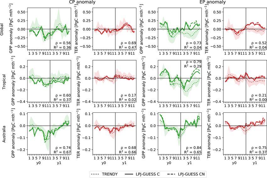
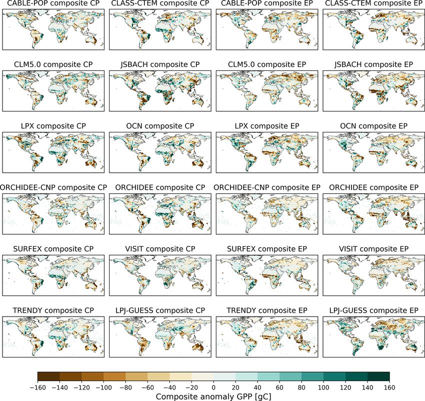
L. Teckentrup et al.: Examining the sensitivity of the terrestrial carbon cycle                                                   2187

Figure 3. Absolute difference and cumulative sums of the difference between CP-only scenario and control climate and EP-only scenario
and control climate for gross primary production (GPP), terrestrial ecosystem respiration (TER, the sum of autotrophic and heterotrophic
respiration) and fire carbon emissions (Fire).

similar to many land surface and dynamic global vegetation            ferent expressions of El Niño in the carbon cycle similarly to
models, does not account for acclimation of plant respira-            other models. We used the TRENDY v7 S2 run with transient
tion to increased temperature and may consequently overes-            CO2 forcing and climate, but no imposed land use change.
timate the carbon sensitivity to temperature changes on short         We choose the seven state-of-the-art DGVMs CABLE-POP
timescales (e.g. Wang et al., 2020; Huntingford et al., 2017;         (Haverd et al., 2018), CLASS–CTEM (Melton and Arora,
Smith et al., 2015). Similarly, models differ in their sensi-         2016), CLM5.0 (Oleson et al., 2013), JSBACH (Reick et al.,
tivity of the carbon cycle as water becomes limiting (Powell          2013), LPX (Keller et al., 2017), OCN (Zaehle and Friend,
et al., 2013), which may affect the magnitude of carbon up-           2010), ORCHIDEE (Krinner et al., 2005), ORCHIDEE-CNP
take in extreme El Niño years. Fisher et al. (2018) also high-        (Goll et al., 2017), SURFEX (Boone et al., 2012) and VISIT
lighted hydrodynamics as well as the representation of de-            (Kato et al., 2013) to calculate the TRENDY composite.
mographic processes (e.g. recruitment and mortality) and fire         LPJ-GUESS matches the TRENDY composite well for GPP
disturbance as areas of uncertainty and promising for model           and TER for the global, tropical and Australian averages,
development. Future experiments will also need to explore             with high correlation coefficients for the global and Aus-
how rising CO2 and temperature change the relative balance            tralian averages (0.52–0.84) and low-to-moderate correlation
of GPP uptake and carbon losses via respiration during El             coefficients for the tropics (0.17–0.6) except for the GPP
Niño events. Wang et al. (2018) showed that the TRENDY                anomaly associated with EP El Niño events (0.79) (see Ap-
model ensemble (which includes an LPJ family member)                  pendix Fig. B10). Similarly, the R 2 values are low for all
generally captured the NBP anomalies associated with CP               tropical anomalies and global EP anomalies (0–0.37), and
El Niño events and only underestimates the anomalies asso-            low to moderate for the remaining regions (0.36–0.67). In
ciated with extreme EP El Niño events. This suggests results          general, LPJ-GUESS displayed greater variability than the
obtained with LPJ-GUESS would be broadly consistent with              TRENDY composite but is mostly within the model range
other DGVMs.                                                          (except for the GPP anomaly for EP El Niños; see Appendix
   To place our results into a broader context, we examined           Fig. B10). The spatial distribution of the composite anoma-
whether LPJ-GUESS captures anomalies associated with dif-             lies shows that LPJ-GUESS captures the features of anoma-

https://doi.org/10.5194/bg-18-2181-2021                                                       Biogeosciences, 18, 2181–2203, 2021
2188                                            L. Teckentrup et al.: Examining the sensitivity of the terrestrial carbon cycle

Figure 4. Absolute difference between CP-only scenario and control climate and EP-only scenario and control climate for the total, vegeta-
tion, litter and soil carbon pools.

lies in GPP associated with EP El Niño events compared                 less direct proxies of variability, such as leaf area index (Zhu
to the individual models and the TRENDY model ensem-                   et al., 2013) and/or GRACE terrestrial water storage (Rodell
ble (see Appendix Fig. B11). In contrast, LPJ-GUESS gen-               et al., 2004).
erally simulates weaker anomalies in GPP associated with                  A further research path may consider driving a model
CP El Niño events in Brazil and western Africa compared                with a larger ensemble of meteorological forcing to account
to the ensemble mean and most individual models. This low              for uncertainties associated with global climate reanalysis
sensitivity might also explain the relatively low correlation          products. We conducted the same experiment based on the
and R 2 values in Appendix Fig. B10 for tropical regions and           GSWP3 climate forcing and found that the overall variabil-
may dampen the overall response to the CP-only scenario.               ity in all terrestrial ecosystem flux and carbon pool anomalies
We note however that LPJ-GUESS still is within the model               is similar to the experiment based on the CRUNCEP dataset
range and can therefore be viewed as representative. In addi-          but with a smaller magnitude (see Appendix Figs. B8 and
tion, LPJ-GUESS has a strong negative bias in Australia. As            B9). Wu et al. (2017) showed that the simulated GPP by
our results show, Australia does not make a large contribution         LPJ-GUESS could vary by as much as 11 PgC yr−1 glob-
to long-term changes in any of the carbon fluxes and pools.            ally, due to the use of alternative climate forcing datasets.
We also examined the sensitivity of our results to the use of          Nevertheless, in their analysis Wu et al. (2017) showed that,
a nitrogen cycle with LPJ-GUESS (see Appendix Fig. B10)                overall, the magnitude of tropical GPP was largely robust to
but did not find a strong sensitivity, most likely because ni-         the use of different precipitation forcing, although there was
trogen is not thought to be strongly limiting in the tropics           variation regionally. Moreover, exploring the impact of dif-
(Vitousek, 1984). Based on this analysis, we suggest that our          ferent expressions of El Niño in a future climate would be
model sensitivity would likely be similar to that displayed by         worthwhile. However, we note that this would probably re-
the other TRENDY models, although we would anticipate                  quire multiple DGVMs to account for the uncertainty asso-
subtle regional differences, particular in the tropics if an al-       ciated with the vegetation responses to CO2 and interactions
ternative DGVM had been used. Especially for EP El Niño                with nutrients (Zaehle et al., 2014). In addition, the represen-
events, LPJ-GUESS diverges from the TRENDY ensemble                    tation of ENSO diversity in CMIP5 and CMIP6 models is
mean, which cannot be explained by nutrient limitation and             highly uncertain due to model biases, especially in the equa-
suggests a different sensitivity to the meteorological drivers         torial Pacific, resulting in low model agreement (e.g. Freund
(see Appendix Fig. B10). Lastly, a comparison with satellite-          et al., 2020). Therefore, to obtain robust results, a future ex-
derived observations might help to estimate whether LPJ-               perimental design would also require an ensemble of climate
GUESS or indeed an alternative DGVM captures the correct               forcing input datasets.
sensitivity in the response of vegetation dynamics to ENSO                In this study, we run LPJ-GUESS with active stochastic
events. Nevertheless, as direct global measurements of car-            and fire disturbance. Including these two types of disturbance
bon fluxes do not exist, and those that do are often based on          contributes significantly to the spatial variability (compare
models themselves, future work might restrict comparison to            Appendix Figs. B1 and B2). Our results show that the fire

Biogeosciences, 18, 2181–2203, 2021                                                        https://doi.org/10.5194/bg-18-2181-2021
L. Teckentrup et al.: Examining the sensitivity of the terrestrial carbon cycle                                              2189

patterns in LPJ-GUESS are largely insensitive to the imposed       5   Conclusions
changes due to the expression of El Niño, which is in contrast
with observational studies that suggest that El Niño events        We explored the impact of the expression of El Niño on
themselves are strongly linked to fire activity on regional        the terrestrial carbon cycle on multi-decadal timescales us-
scales (e.g. Pan et al., 2018; Mariani et al., 2016; Harris and    ing LPJ-GUESS. We found that the changes in simulated
Lucas, 2019; Fonseca et al., 2017). This might result from         anomalies reflecting the two expressions of El Niño in NBP
changes imposed in the experiment being too small to trigger       accumulate around 9.6 PgC (CP-only scenario) and 4.5 PgC
changes in fire patterns. We note however that the fire module     (EP-only scenario). However, this accumulation period cov-
implemented in LPJ-GUESS (LPJ-GUESS–GlobFIRM; see                  ers more than 45 years and is therefore negligible compared
Thonicke et al., 2001) is a relatively simple empirical model      to annual anthropogenic emissions of 9.4 ± 0.5 PgC yr−1
that does not capture observed fire properties well (Hantson       (Le Quéré et al., 2018). Our results therefore suggest that
et al., 2020) and might underestimate the sensitivity of fire      the impact of different expressions of El Niño on the carbon
occurrence to different expressions of El Niño. Teckentrup         cycle on long timescales is likely to be small.
et al. (2019) highlighted notable differences among seven             Our results imply that simulations of the terrestrial carbon
DGVMs in the pattern of burned area to climate forcing. Our        cycle over the recent past and into the future using global
results suggest that the interaction between the expression of     climate models may not require the expression of El Niño
El Niño and fire requires further investigation.                   events to be well captured. There are major challenges in ac-
   Finally, isolating the effect of El Niño on the atmosphere      curately capturing El Niño–La Niña cycles and the telecon-
and terrestrial biosphere is not trivial for individual events.    nections associated with El Niño events with existing climate
Individual El Niño events vary in location, timing and mag-        models. Had we found the expression of El Niño to be criti-
nitude (e.g. Capotondi et al., 2015), and teleconnections are      cal in simulating the long-term terrestrial carbon balance, this
influenced by the background climate and climate variabil-         would have added a very significant additional uncertainty to
ity (e.g. the Indian Ocean Dipole). In our study, we assume        projections of the future role of the land in storing carbon.
that replacing a CP event with an EP event, or vice versa,         Our results suggest that the expression of El Niño, as distinct
did not modify the role played by other modes of variability.      from whether there is an El Niño or a La Niña, is relatively
We further neglect possible interactions between consecutive       unimportant over the long term. We note that our results do
ENSO events. For example, strong El Niño events tend to            agree with earlier studies (Chylek et al., 2018; Wang et al.,
peak in the eastern Pacific, and these tend to be followed by      2018; Pan et al., 2018) that found that the expression of El
a La Niña event. However, the influence of a preceding El          Niño is important to terrestrial carbon fluxes on shorter, an-
Niño on the characteristics of the La Niña event is not clear      nual and interannual timescales. Overall, in the context of the
(Santoso et al., 2017). By generating two experiments with         long-term global and regional terrestrial carbon balance, our
either 15 (nine manipulated events) CP or 15 (eight manip-         results imply that model development should prioritise sim-
ulated events) EP El Niño events, we assume that the signal        ulating El Niño–La Niña cycles and the associated telecon-
observed at the end of the time period is driven by the respec-    nections, with perhaps less focus needed on considering the
tive expression of El Niño. In order to test the validity of our   additional challenge of resolving the expression of individual
results, we applied a different approach where we replaced         El Niño events.
the climate forcing of CP El Niño years with the climate forc-
ing of the EP El Niño events closest in time and found even
smaller changes in carbon fluxes (see Appendix Fig. B6) and
in carbon sequestration (see Appendix Fig. B7). An alterna-
tive approach could be to calculate composite anomalies for
both CP and EP El Niño events and use those for replace-
ment, but this would dampen variability in the forcing and
introduce a different bias. Alternatively, generating a sea sur-
face temperature forcing representing the different expres-
sions of El Niño and using an atmospheric model to gener-
ate the climate anomalies that result from the changes in sea
surface temperatures could help quantify the effect of the ex-
pression of El Niño on the carbon sequestration. However,
given the changes we found are very small and spatially vari-
able, we doubt this would lead to different conclusions.

https://doi.org/10.5194/bg-18-2181-2021                                                   Biogeosciences, 18, 2181–2203, 2021
2190 L. Teckentrup et al.: Examining the sensitivity of the terrestrial carbon cycle
Appendix A
Table A1. El Niño events from 1968–2010 identified by the NOAA Oceanic Niño Index (ONI) and their different expressions derived by four
methods according to Yu and Kim (2013): pattern correlation method (“PTN”; Yu and Kim, 2013); central location method (“Niño”; Kug
et al., 2009; Yeh et al., 2009), the El Niño Modoki index (“EMI”; Ashok et al., 2007), and the cold-tongue and warm-pool index (“CT/WP”;
Ren and Jin, 2011). We define a CP or EP El Niño where three out of the four indices agree on the same El Niño type. The remaining events
are defined as mixed events (“MIX”).
Year Dominant CP El Niño EP El Niño
El Niño type replacement replacement
1968–1969 CP – 1976–1977
1969–1970 EP 1977–1978 –
1972–1973 EP 2009–2010 –
1976–1977 EP 1977–1978 –
1977–1978 CP – 1976–1977
1982–1983 EP 2009–2010 –
1986–1987 EP 1994–1995 –
1987–1988 MIX 2002–2003 1982–1983
1991–1992 MIX 2009–2010 1997–1998
1994–1995 CP – 1976–1977
1997–1998 EP 2002–2003 –
2002–2003 CP – 2006–2007
2004–2005 CP – 1976–1977
2006–2007 EP 1977–1978 –
2009–2010 CP – 1972–1973
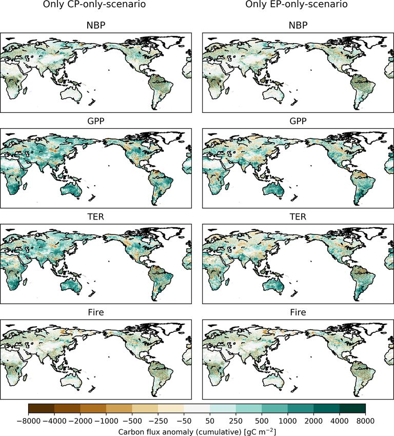
Biogeosciences, 18, 2181–2203, 2021 https://doi.org/10.5194/bg-18-2181-2021L. Teckentrup et al.: Examining the sensitivity of the terrestrial carbon cycle 2191 Appendix B B1 CRUNCEP Figure B1. Absolute difference between CP-only scenario and control climate and EP-only scenario and control climate for net biome production (NBP), gross primary production (GPP), terrestrial ecosystem respiration (TER) and fire carbon emissions (Fire) for the final year of the experiment (2013). Note that the noise partially results from stochastic and fire disturbance (compare Fig. B2). https://doi.org/10.5194/bg-18-2181-2021 Biogeosciences, 18, 2181–2203, 2021
2192                                             L. Teckentrup et al.: Examining the sensitivity of the terrestrial carbon cycle

Figure B2. Absolute difference between CP-only scenario and control climate and EP-only scenario and control climate for net biome
production (NBP), gross primary production (GPP), terrestrial ecosystem respiration (TER) and fire carbon emissions (Fire) for the final year
of the experiment (2013) without stochastic and fire disturbance.

Biogeosciences, 18, 2181–2203, 2021                                                          https://doi.org/10.5194/bg-18-2181-2021
L. Teckentrup et al.: Examining the sensitivity of the terrestrial carbon cycle                                                   2193

Figure B3. Accumulated absolute difference between CP-only scenario and control climate and EP-only scenario and control climate for net
biome production (NBP), gross primary production (GPP), terrestrial ecosystem respiration (TER) and fire carbon emissions (Fire) for the
final year of the experiment (2013).

https://doi.org/10.5194/bg-18-2181-2021                                                       Biogeosciences, 18, 2181–2203, 2021
2194                                             L. Teckentrup et al.: Examining the sensitivity of the terrestrial carbon cycle

Figure B4. Absolute difference between CP-only scenario and control climate and EP-only scenario and control climate for total, vegetation,
litter and soil carbon pool for the final year of the experiment (2013).

Biogeosciences, 18, 2181–2203, 2021                                                         https://doi.org/10.5194/bg-18-2181-2021
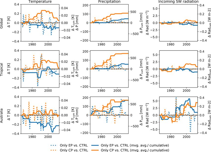
L. Teckentrup et al.: Examining the sensitivity of the terrestrial carbon cycle                                                  2195

Figure B5. Absolute difference and cumulative sums of the difference between CP-only scenario and control climate and EP-only scenario
and control climate for precipitation and absolute difference and 30-year moving average of the difference between CP-only scenario and
control climate and EP-only scenario and control climate for temperature and incoming shortwave radiation.

https://doi.org/10.5194/bg-18-2181-2021                                                       Biogeosciences, 18, 2181–2203, 2021
2196                                             L. Teckentrup et al.: Examining the sensitivity of the terrestrial carbon cycle

B2     Nearest-year replacement

Figure B6. Absolute difference and cumulative sums of the difference between CP-only scenario and control climate and EP-only scenario
and control climate for net biome production (NBP), gross primary production (GPP), terrestrial ecosystem respiration (TER, the sum of
autotrophic and heterotrophic respiration) and fire carbon emissions (Fire) for an alternative method (replacing the climate forcing of CP El
Niño event with that of an EP El Niño event and vice versa for events closest in time).

Figure B7. Absolute difference between CP-only scenario and control climate and EP-only scenario and control climate for the total,
vegetation, litter and soil carbon pools for an alternative method (replacing the climate forcing of CP El Niño event with that of an EP El
Niño event and vice versa for events closest in time).

Biogeosciences, 18, 2181–2203, 2021                                                          https://doi.org/10.5194/bg-18-2181-2021
L. Teckentrup et al.: Examining the sensitivity of the terrestrial carbon cycle                                                 2197

B3   GSWP3 forcing

Figure B8. Absolute difference and cumulative sums of the difference between CP-only scenario and control climate and EP-only scenario
and control climate for net biome production (NBP), gross primary production (GPP), terrestrial ecosystem respiration (TER, the sum of
autotrophic and heterotrophic respiration) and fire carbon emissions (Fire) for the experiments based on the GSWP3 forcing.

Figure B9. Absolute difference between CP-only scenario and control climate and EP-only scenario and control climate for the total,
vegetation, litter and soil carbon pools for the experiments based on the GSWP3 forcing.

https://doi.org/10.5194/bg-18-2181-2021                                                      Biogeosciences, 18, 2181–2203, 2021
2198                                              L. Teckentrup et al.: Examining the sensitivity of the terrestrial carbon cycle

Figure B10. Monthly composite anomalies during the El Niño developing (y0 ) and decaying (y1 ) year in gross primary production (GPP,
green lines) and terrestrial ecosystem respiration (TER, sum of autotrophic and heterotrophic respiration, red lines) for all CP and EP El Niño
events listed in Appendix Table A1 averaged over the globe, the tropics (23◦ S–23◦ N) and Australia. The dotted lines show the TRENDY
v7 composite, the solid lines are the individual LPJ-GUESS runs without nitrogen cycling (“LPJ-GUESS C”) and the dashed lines show
the individual LPJ-GUESS runs with nitrogen cycling (“LPJ-GUESS CN”) (compare Wang et al., 2018). The shaded area shows the model
spread of the individual TRENDY models. ρ and R 2 are the Pearson correlation coefficient and the R 2 value, respectively, between the
individual LPJ-GUESS runs without nitrogen cycling and the TRENDY ensemble mean.

Biogeosciences, 18, 2181–2203, 2021                                                           https://doi.org/10.5194/bg-18-2181-2021
L. Teckentrup et al.: Examining the sensitivity of the terrestrial carbon cycle                                            2199

Figure B11. Composite anomalies in gross primary production (GPP) summed over the El Niño developing and decaying year for all CP
and EP El Niño events listed in Table A1 for the individual TRENDY models, the TRENDY composite and the individual LPJ-GUESS run
(compare Wang et al., 2018).

https://doi.org/10.5194/bg-18-2181-2021                                                  Biogeosciences, 18, 2181–2203, 2021
2200                                              L. Teckentrup et al.: Examining the sensitivity of the terrestrial carbon cycle

Code and data availability. The analysis codes are available at           tion over land by increasing the model sensitivity to veg-
https://github.com/lteckentrup/nino_experiment, Teckentrup, 2021.         etation variability in EC-Earth, Clim. Dyn., 49, 1215–1237,
The model code is available upon request from http://web.nateko.lu.       https://doi.org/10.1007/s00382-016-3372-4, 2017.
se/lpj-guess/contact.html, Smith, 2020. The model outputs will be       Ashok, K., Behera, S. K., Rao, S. A., Weng, H., and Yamagata,
shared in line with UNSW’s open-access policy on publication. The         T.: El Niño Modoki and its possible teleconnection, J. Geophys.
TRENDY version 7 model output is available upon request (https:           Res.-Oceans, 112, C11, https://doi.org/10.1029/2006JC003798,
//sites.exeter.ac.uk/trendy/data-policy/, last access: 31 July 2020),     2007.
and the CRUNCEP climate forcing is available from https://rda.          Ashok, K., Iizuka, S., Rao, S. A., Saji, N. H., and Lee, W.-
ucar.edu/datasets/ds314.3/, Viovy, 2018.                                  J.: Processes and boreal summer impacts of the 2004 El
                                                                          Niño Modoki: An AGCM study, Geophys. Res. Lett., 36, 4,
                                                                          https://doi.org/10.1029/2008GL036313, 2009.
Author contributions. LT, MGDK and AJP designed the experi-             Bastos, A., Friedlingstein, P., Sitch, S., Chen, C., Mialon, A.,
ment and performed the model runs and the analysis with input from        Wigneron, J.-P., Arora, V. K., Briggs, P. R., Canadell, J. G.,
BS. LT, MGDK and AJP wrote the paper with contributions from              Ciais, P., Chevallier, F., Cheng, L., Delire, C., Haverd, V., Jain,
BS.                                                                       A. K., Joos, F., Kato, E., Lienert, S., Lombardozzi, D., Melton,
                                                                          J. R., Myneni, R., Nabel, J. E. M. S., Pongratz, J., Poulter, B.,
                                                                          Rödenbeck, C., Séférian, R., Tian, H., van Eck, C., Viovy, N.,
Competing interests. The authors declare that they have no conflict       Vuichard, N., Walker, A. P., Wiltshire, A., Yang, J., Zaehle,
of interest.                                                              S., Zeng, N., and Zhu, D.: Impact of the 2015/2016 El Niño
                                                                          on the terrestrial carbon cycle constrained by bottom-up and
                                                                          top-down approaches, Philos. T. Roy. Soc. B„ 373, 20170304,
                                                                          https://doi.org/10.1098/rstb.2017.0304, 2018.
Acknowledgements. Lina Teckentrup, Martin G. De Kauwe and
                                                                        Bellenger, H., Guilyardi, E., Leloup, J., Lengaigne, M.,
Andrew J. Pitman acknowledge support from the Australian Re-
                                                                          and Vialard, J.: ENSO representation in climate mod-
search Council (ARC) Centre of Excellence for Climate Ex-
                                                                          els: from CMIP3 to CMIP5, Clim. Dyn., 42, 1999–2018,
tremes (CE170100023). Martin G. De Kauwe and Andrew J. Pit-
                                                                          https://doi.org/10.1007/s00382-013-1783-z, 2014.
man acknowledge support from the ARC Discovery Grant
                                                                        Boone, A., Belamari, S., Brun, E., Calvet, J.-C., Decharme, B.,
(DP190101823). Martin G. De Kauwe was also supported from
                                                                          Faroux, S., Gibelin, A.-L., Giordani, H., Lafont, S., Lebeaupin,
the NSW Research Attraction and Acceleration Program. We fur-
                                                                          C., Le Moigne, P., Mahfouf, J.-F., Martin, E., Masson, V.,
ther acknowledge the TRENDY DGVM community, as part of the
                                                                          Mironov, D., Morin, S., Noilhan, J., Tulet, P., Van Den Hurk, B.,
Global Carbon Project, for access to their model outputs. We thank
                                                                          and Vionnet, V.: SURFEX scientific documentation, SURFEX
the National Computational Infrastructure at the Australian Na-
                                                                          v7.2 – Issue no2 – 2012, 2012.
tional University, an initiative of the Australian Government, for
                                                                        Cai, W., Wang, G., Dewitte, B., Wu, L., Santoso, A., Takahashi, K.,
access to supercomputer resources. Finally, we thank Matthew For-
                                                                          Yang, Y., Carréric, A., and McPhaden, M. J.: Increased variabil-
rest for his support in running LPJ-GUESS.
                                                                          ity of eastern Pacific El Niño under greenhouse warming, Na-
                                                                          ture, 564, 201–206, https://doi.org/10.1038/s41586-018-0776-9,
                                                                          2018.
Financial support. This research has been supported by the Aus-         Capotondi, A., Wittenberg, A. T., Newman, M., Di Lorenzo, E., Yu,
tralian Research Council (ARC) Centre of Excellence for Climate           J.-Y., Braconnot, P., Cole, J., Dewitte, B., Giese, B., Guilyardi,
Extremes (grant no. CE170100023) and the ARC Discovery Grant              E., Jin, F.-F., Karnauskas, K., Kirtman, B., Lee, T., Schneider, N.,
(grant no. DP190101823).                                                  Xue, Y., and Yeh, S.-W.: Understanding ENSO Diversity, B. Am.
                                                                          Meteorol. Soc., 96, 921–938, https://doi.org/10.1175/BAMS-D-
                                                                          13-00117.1, 2015.
Review statement. This paper was edited by Alexandra Konings            Chylek, P., Tans, P., Christy, J., and Dubey, M. K.: The carbon
and reviewed by Jun Wang and two anonymous referees.                      cycle response to two El Niño types: an observational study,
                                                                          Environ. Res. Lett., 13, 024001, https://doi.org/10.1088/1748-
                                                                          9326/aa9c5b, 2018.
                                                                        Compo, G. P., Whitaker, J. S., Sardeshmukh, P. D., Matsui, N., Al-
References                                                                lan, R. J., Yin, X., Gleason, B. E., Vose, R. S., Rutledge, G.,
                                                                          Bessemoulin, P., Brönnimann, S., Brunet, M., Crouthamel, R. I.,
Ahlström, A., Raupach, M. R., Schurgers, G., Smith, B., Arneth,           Grant, A. N., Groisman, P. Y., Jones, P. D., Kruk, M. C., Kruger,
  A., Jung, M., Reichstein, M., Canadell, J. G., Friedlingstein,          A. C., Marshall, G. J., Maugeri, M., Mok, H. Y., Nordli, Ø., Ross,
  P., Jain, A. K., Kato, E., Poulter, B., Sitch, S., Stocker, B. D.,      T. F., Trigo, R. M., Wang, X. L., Woodruff, S. D., and Worley,
  Viovy, N., Wang, Y. P., Wiltshire, A., Zaehle, S., and Zeng,            S. J.: The Twentieth Century Reanalysis Project, Q. J. Roy. Me-
  N.: The dominant role of semi-arid ecosystems in the trend              teor. Soc., 137, 1–28, https://doi.org/10.1002/qj.776, 2011.
  and variability of the land CO2 sink, Science, 348, 895–899,          Donguy, J.-R. and Dessier, A.: El Niño-Like Events
  https://doi.org/10.1126/science.aaa1668, 2015.                          Observed in the Tropical Pacific, Mon. Weather
Alessandri, A., Catalano, F., De Felice, M., Van Den Hurk,                Rev.,       111,     2136–2139,      https://doi.org/10.1175/1520-
  B., Doblas Reyes, F., Boussetta, S., Balsamo, G., and                   0493(1983)1112.0.CO;2, 1983.
  Miller, P. A.: Multi-scale enhancement of climate predic-

Biogeosciences, 18, 2181–2203, 2021                                                         https://doi.org/10.5194/bg-18-2181-2021
L. Teckentrup et al.: Examining the sensitivity of the terrestrial carbon cycle 2201 Fang, Y., Michalak, A. M., Schwalm, C. R., Huntzinger, D. N., Ecol. Biogeogr., 21, 50–63, https://doi.org/10.1111/j.1466- Berry, J. A., Ciais, P., Piao, S., Poulter, B., Fisher, J. B., 8238.2010.00613.x, 2012. Cook, R. B., Hayes, D., Huang, M., Ito, A., Jain, A., Lei, H., Huntingford, C., Atkin, O., Martínez-de la Torre, A., Mercado, Lu, C., Mao, J., Parazoo, N. C., Peng, S., Ricciuto, D. M., L., Heskel, M. A., Harper, A. B., Bloomfield, K., O’Sullivan, Shi, X., Tao, B., Tian, H., Wang, W., Wei, Y., and Yang, J.: O., Reich, P., Wythers, K., Butler, E., Chen, M., Griffin, K., Global land carbon sink response to temperature and precipita- Meir, P., Tjoelker, M., Turnbull, M., Sitch, S., Wiltshire, A., tion varies with ENSO phase, Environ. Res. Lett., 12, 064007, and Malhi, Y.: Implications of improved representations of plant https://doi.org/10.1088/1748-9326/aa6e8e, 2017. respiration in a changing climate, Nat. Commun., 8, 1602, Fisher, R. A., Koven, C. D., Anderegg, W. R. L., Christoffersen, https://doi.org/10.1038/s41467-017-01774-z, 2017. B. O., Dietze, M. C., Farrior, C. E., Holm, J. A., Hurtt, G. C., Kato, E., Kinoshita, T., Ito, A., Kawamiya, M., and Yama- Knox, R. G., Lawrence, P. J., Lichstein, J. W., Longo, M., Ma- gata, Y.: Evaluation of spatially explicit emission scenario theny, A. M., Medvigy, D., Muller-Landau, H. C., Powell, T. L., of land-use change and biomass burning using a process- Serbin, S. P., Sato, H., Shuman, J. K., Smith, B., Trugman, A. T., based biogeochemical model, J. Land Use Sci., 8, 104–122, Viskari, T., Verbeeck, H., Weng, E., Xu, C., Xu, X., Zhang, T., https://doi.org/10.1080/1747423X.2011.628705, 2013. and Moorcroft, P. R.: Vegetation demographics in Earth System Keller, K. M., Lienert, S., Bozbiyik, A., Stocker, T. F., Chu- Models: A review of progress and priorities, Glob. Change Biol., rakova (Sidorova), O. V., Frank, D. C., Klesse, S., Koven, C. 24, 35–54, https://doi.org/10.1111/gcb.13910, 2018. D., Leuenberger, M., Riley, W. J., Saurer, M., Siegwolf, R., Fonseca, M. G., Anderson, L. O., Arai, E., Shimabukuro, Y. E., Weigt, R. B., and Joos, F.: 20th century changes in carbon Xaud, H. A. M., Xaud, M. R., Madani, N., Wagner, F. H., and isotopes and water-use efficiency: tree-ring-based evaluation of Aragão, L. E. O. C.: Climatic and anthropogenic drivers of north- the CLM4.5 and LPX-Bern models, Biogeosciences, 14, 2641– ern Amazon fires during the 2015–2016 El Niño event, Ecol. 2673, https://doi.org/10.5194/bg-14-2641-2017, 2017. Appl., 27, 2514–2527, https://doi.org/10.1002/eap.1628, 2017. Kelley, D. and Harrison, S.: Enhanced Australian carbon sink Freund, M. B., Brown, J. R., Henley, B. J., Karoly, D. J., and despite increased wildfire during the 21st century, En- Brown, J. N.: Warming Patterns Affect El Niño Diversity viron. Res. Lett., 9, 104015, https://doi.org/10.1088/1748- in CMIP5 and CMIP6 Models, J. Climate, 33, 8237–8260, 9326/9/10/104015, 2014. https://doi.org/10.1175/JCLI-D-19-0890.1, 2020. Kim, H.: Global Soil Wetness Project Phase 3 Atmospheric Bound- Goll, D. S., Vuichard, N., Maignan, F., Jornet-Puig, A., Sar- ary Conditions (Experiment 1), Data Integration and Analysis dans, J., Violette, A., Peng, S., Sun, Y., Kvakic, M., Guim- System (DIAS), https://doi.org/10.20783/DIAS.501, 2017. berteau, M., Guenet, B., Zaehle, S., Penuelas, J., Janssens, I., Kim, J.-S., Kug, J.-S., Yoon, J.-H., and Jeong, S.-J.: Increased atmo- and Ciais, P.: A representation of the phosphorus cycle for OR- spheric CO2 growth rate during El Niño driven by reduced ter- CHIDEE (revision 4520), Geosci. Model Dev., 10, 3745–3770, restrial productivity in the CMIP5 ESMs, J. Climate, 29, 8783– https://doi.org/10.5194/gmd-10-3745-2017, 2017. 8805, https://doi.org/10.1175/JCLI-D-14-00672.1, 2016. Hantson, S., Kelley, D. I., Arneth, A., Harrison, S. P., Archibald, S., Kim, J.-S., Kug, J.-S., and Jeong, S.-J.: Intensification of ter- Bachelet, D., Forrest, M., Hickler, T., Lasslop, G., Li, F., Man- restrial carbon cycle related to El Niño-Southern Oscilla- geon, S., Melton, J. R., Nieradzik, L., Rabin, S. S., Prentice, I. tion under greenhouse warming, Nat. Commun., 8, 1674, C., Sheehan, T., Sitch, S., Teckentrup, L., Voulgarakis, A., and https://doi.org/10.1038/s41467-017-01831-7, 2017. Yue, C.: Quantitative assessment of fire and vegetation properties Krinner, G., Viovy, N., de Noblet-Ducoudré, N., Ogée, J., Polcher, in simulations with fire-enabled vegetation models from the Fire J., Friedlingstein, P., Ciais, P., Sitch, S., and Prentice, I. C.: Model Intercomparison Project, Geosci. Model Dev., 13, 3299– A dynamic global vegetation model for studies of the coupled 3318, https://doi.org/10.5194/gmd-13-3299-2020, 2020. atmosphere-biosphere system, Global Biogeochem. Cy., 19, 1, Harris, S. and Lucas, C.: Understanding the variability of Australian https://doi.org/10.1029/2003GB002199, 2005. fire weather between 1973 and 2017, Plos One, 14, e0222328, Kug, J.-S., Jin, F.-F., and An, S.-I.: Two Types of El Niño Events: https://doi.org/10.1371/journal.pone.0222328, 2019. Cold Tongue El Niño and Warm Pool El Niño, J. Climate, 22, Haverd, V., Ahlström, A., Smith, B., and Canadell, J. G.: 1499–1515, https://doi.org/10.1175/2008JCLI2624.1, 2009. Carbon cycle responses of semi-arid ecosystems to posi- Le Quéré, C., Andrew, R. M., Friedlingstein, P., Sitch, S., Hauck, tive asymmetry in rainfall, Glob. Change Biol., 23, 793–800, J., Pongratz, J., Pickers, P. A., Korsbakken, J. I., Peters, G. P., https://doi.org/10.1111/gcb.13412, 2017. Canadell, J. G., Arneth, A., Arora, V. K., Barbero, L., Bastos, Haverd, V., Smith, B., Nieradzik, L., Briggs, P. R., Woodgate, W., A., Bopp, L., Chevallier, F., Chini, L. P., Ciais, P., Doney, S. C., Trudinger, C. M., Canadell, J. G., and Cuntz, M.: A new version Gkritzalis, T., Goll, D. S., Harris, I., Haverd, V., Hoffman, F. M., of the CABLE land surface model (Subversion revision r4601) Hoppema, M., Houghton, R. A., Hurtt, G., Ilyina, T., Jain, A. incorporating land use and land cover change, woody vegetation K., Johannessen, T., Jones, C. D., Kato, E., Keeling, R. F., Gold- demography, and a novel optimisation-based approach to plant ewijk, K. K., Landschützer, P., Lefèvre, N., Lienert, S., Liu, Z., coordination of photosynthesis, Geosci. Model Dev., 11, 2995– Lombardozzi, D., Metzl, N., Munro, D. R., Nabel, J. E. M. S., 3026, https://doi.org/10.5194/gmd-11-2995-2018, 2018. Nakaoka, S., Neill, C., Olsen, A., Ono, T., Patra, P., Peregon, Hickler, T., Vohland, K., Feehan, J., Miller, P. A., Smith, B., A., Peters, W., Peylin, P., Pfeil, B., Pierrot, D., Poulter, B., Re- Costa, L., Giesecke, T., Fronzek, S., Carter, T. R., Cramer, W., hder, G., Resplandy, L., Robertson, E., Rocher, M., Rödenbeck, Kühn, I., and Sykes, M. T.: Projecting the future distribution C., Schuster, U., Schwinger, J., Séférian, R., Skjelvan, I., Stein- of European potential natural vegetation zones with a gener- hoff, T., Sutton, A., Tans, P. P., Tian, H., Tilbrook, B., Tubiello, alized, tree species-based dynamic vegetation model, Global F. N., van der Laan-Luijkx, I. T., van der Werf, G. R., Viovy, N., https://doi.org/10.5194/bg-18-2181-2021 Biogeosciences, 18, 2181–2203, 2021
You can also read