Atlantic hurricane response to Saharan greening and reduced dust emissions during the mid-Holocene - CP
←
→
Page content transcription
If your browser does not render page correctly, please read the page content below
Clim. Past, 17, 675–701, 2021
https://doi.org/10.5194/cp-17-675-2021
© Author(s) 2021. This work is distributed under
the Creative Commons Attribution 4.0 License.

Atlantic hurricane response to Saharan greening and reduced
dust emissions during the mid-Holocene
Samuel Dandoy1,a , Francesco S. R. Pausata1 , Suzana J. Camargo2 , René Laprise1 , Katja Winger1 , and
Kerry Emanuel3
1 Department   of Earth and Atmospheric Sciences, Université du Québec à Montréal, Montreal, Quebec, Canada
2 Lamont-Doherty    Earth Observatory, Columbia University, Palisades, NY, USA
3 Program in Atmospheres, Oceans, and Climate, Department of Earth, Atmospheric, and Planetary Sciences, Massachusetts

Institute of Technology, Cambridge, MA, USA
a now at: Canadian Meteorological Aviation Centre, Environment and Climate Change Canada, Montreal, Quebec, Canada

Correspondence: Samuel Dandoy (dandoii@hotmail.ca)

Received: 28 August 2020 – Discussion started: 22 September 2020
Accepted: 22 January 2021 – Published: 25 March 2021

Abstract. We use a high-resolution regional climate model        1   Introduction
to investigate the changes in Atlantic tropical cyclone
(TC) activity during the period of the mid-Holocene (MH:
6000 years BP) with a larger amplitude of the seasonal cycle     Tropical cyclones (TCs) are one of the most powerful atmo-
relative to today. This period was characterized by increased    spheric phenomena on Earth. With increasing damages and
boreal summer insolation over the Northern Hemisphere, a         costs due to natural disasters and recent upswing in Atlantic
vegetated Sahara and reduced airborne dust concentrations.       TCs, it becomes more and more important to understand how
A set of sensitivity experiments was conducted in which solar    TC activity may change in the future. As TC development
insolation, vegetation and dust concentrations were changed      is strongly influenced by, among others, vertical wind shear,
in turn to disentangle their impacts on TC activity in the       sea surface temperature (SST) and humidity, changes in these
Atlantic Ocean. Results show that the greening of the Sa-        environmental parameters due to climate change may result
hara and reduced dust loadings (MHGS+RD ) lead to a larger       in large variability in TC activity. The ongoing global warm-
increase in the number of Atlantic TCs (27 %) relative to        ing can affect those environmental variables both directly by
the pre-industrial (PI) climate than the orbital forcing alone   increasing the SST and indirectly through changes in the at-
(MHPMIP ; 9 %). The TC seasonality is also highly modified       mospheric stability and circulation. A recent study (Evan et
in the MH climate, showing a decrease in TC activity dur-        al., 2016) has shown that changes in atmospheric circulation
ing the beginning of the hurricane season (June to August),      at the end of the century could potentially reduce dust load-
with a shift of its maximum towards October and Novem-           ings over the tropical North Atlantic by around 10 %. Evan et
ber in the MHGS+RD experiment relative to PI. MH experi-         al. (2006) showed that Saharan dust layer is strongly linked
ments simulate stronger hurricanes compared to PI, similar       to changes in North Atlantic TC activity, acting as an inhibit-
to future projections. Moreover, they suggest longer-lasting     ing factor for TC formation, as also previously suggested by
cyclones relative to PI. Our results also show that changes      Dunion and Velden (2004). These studies suggest that reduc-
in the African easterly waves are not relevant in altering the   ing the Saharan dust layer could lead to an increase in TC
frequency and intensity of TCs, but they may shift the loca-     genesis occurrence, as well as more intense TCs by changes
tion of their genesis. This work highlights the importance of    in the midlevel jet, directly impacting the vertical wind shear,
considering vegetation and dust changes over the Sahara re-      and by increasing incoming solar radiation at the surface,
gion when investigating TC activity under a different climate    directly warming the ocean surface. Local changes in the
state.                                                           energy fluxes could also affect the atmospheric circulation
                                                                 through changes in the position of the Intertropical Conver-

Published by Copernicus Publications on behalf of the European Geosciences Union.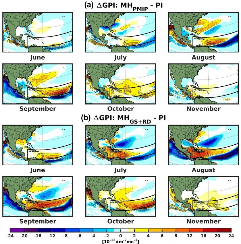
676                                                                S. Dandoy et al.: Atlantic hurricane response during the MH

gence Zone (ITCZ) or the West African monsoon (WAM) af-             modeling simulations as in Pausata et al. (2017) to drive a
fecting TC activity (Schneider et al., 2014; Seth et al., 2019).    high-resolution regional climate model to investigate the im-
For these reasons, a better understanding of the role of WAM        pact of the atmospheric dynamics changes induced by Sa-
intensity and dust loading in altering hurricane activity is of     haran vegetation and dust reduction on TC activity during
paramount importance.                                               the MH compared to the PI climate. This study will compare
   Dramatic intensifications of the WAM have occurred in            the dynamical downscaling results to those obtained with the
the past (Shanahan et al., 2009), the most recent during the        statistical thermodynamical downscaling approach used by
early and middle Holocene (MH, 12 000–5000 years BP),               Pausata et al. (2017) and how they compare with the find-
when the WAM was much stronger and extended further in-             ings of Koh and Brierley (2015) and Korty et al. (2012). It
land than today. The northward penetration of the WAM led           will also provide insights into how a potential warmer and
to an expansion of the northern African lakes and wetlands,         greener Northern Hemisphere could alter future Atlantic TC
as well as to an extension of Sahelian vegetation into areas        activity.
that are now desert, giving origin to the so-called “green Sa-         The paper is structured as follows. The model description,
hara” (e.g., Holmes, 2008; Kowalski et al., 1989; Rohling           experimental design and the analytical tools used in the study
et al., 2004). Therefore, the MH climate represents a good          are presented in Sect. 2. Section 3 focuses on (1) the model’s
test case to investigate the TC response to changes in orbital      response to the changes in climate conditions on TC activity,
forcing and also investigate how radiative forcing caused by        (2) the seasonal distribution of TCs and (3) their intensity.
a greener Northern Hemisphere can impact their genesis.             Discussion and conclusions are presented in Sect. 4.
   Paleotempestology records are, however, sparse and most
of them only span a few millennia, making it difficult to eval-
                                                                    2     Model description and methodology
uate TC variability further back than the observational pe-
riod. Nevertheless, records from the western North Atlantic         2.1    Models
suggest large variations in the frequency of hurricane land-
falls during the late Holocene, together with strong positive       The simulations carried out by Pausata et al. (2016) and
anomalies in the WAM (Donnelly and Woodruff, 2007; Greer            Gaetani et al. (2017) and performed with an Earth sys-
and Swart, 2006; Liu and Fearn, 2000; Toomey et al., 2013).         tem model (EC-Earth version 3.1) at horizontal resolution
   Only a handful of modeling studies investigating TC              of 1.125◦ × 1.125◦ and 62 levels in the vertical for the at-
changes during the MH are currently available (Korty et             mosphere (Hazeleger et al., 2012) are used in this study
al., 2012; Koh and Brierley, 2015; Pausata et al., 2017). Both      to drive a developmental version of the sixth generation
Korty et al. (2012) and Koh and Brierley (2015) have focused        Canadian Regional Climate Model (CRCM6; see Girard et
on simulations of the Paleoclimate Modelling Intercompari-          al., 2014 and McTaggart-Cowan et al., 2019). The exper-
son Project (PMIP), which only account for the change in or-        iments with CRCM6 are carried out on a grid mesh of
bital forcing and the greenhouse gas (GHG) concentrations           0.11◦ . This high-horizontal-resolution grid allows us to cap-
during the MH, assuming pre-industrial vegetation cover and         ture many processes that are related to TC genesis and simu-
dust concentrations. These studies do not explicitly simulate       late intense tropical cyclones (Strachan et al., 2013; Walsh
the changes in TCs but rather investigate how key environ-          et al., 2013; Shaevitz et al., 2014; Camargo and Wing,
mental variables affect TC genesis due to the insolation forc-      2016; Kim et al., 2018; Wing et al., 2019). An additional
ing. Both studies came to similar conclusions that consid-          0.22◦ reference experiment has been performed to evalu-
ering changes in the orbital forcing makes the environment          ate the results against reanalysis and observations. CRCM6
less prone to develop TCs in Northern Hemisphere summer             is derived from the Global Environmental Multiscale ver-
and more prone in the Southern Hemisphere summer. More              sion 4.8 (GEM4.8), an integrated forecasting and data as-
recently, Pausata et al. (2017) used a statistical thermody-        similation system developed by the Recherche en Prévision
namical downscaling approach (Emanuel, 2006; Emanuel et             Numérique (RPN), Meteorological Research Branch (MRB)
al., 2008) to generate a large number of synthetic TCs and          and the Canadian Meteorological Centre (CMC). GEM4.8
assess their changes during the MH with an enhanced vegeta-         is a fully non-hydrostatic model that uses a semi-implicit,
tion cover over the Sahara and reduced airborne dust concen-        semi-Lagrangian time discretization scheme on a horizontal
trations. Their results suggest a large increase in TC activity     Arakawa staggered C grid. It can be run either as a global cli-
worldwide and in particular in the Atlantic Ocean in the MH         mate model (GCM), covering the entire globe, or as a nested
climate. However, this kind of downscaling approach does            regional climate model (RCM). In the RCM configuration,
not consider how the TC genesis may have been affected by           the model uses a hybrid terrain-following vertical coordinate
changes in atmospheric dynamics, such as those associated           with 53 levels topping at 10 hPa. For shallow convection,
with the African easterly waves (AEWs; Gaetani et al., 2017)        GEM uses the Kuo transient scheme (Bélair al., 2005; Kuo,
that are known to seed TC genesis (Caron and Jones, 2012;           1965), and for deep convective processes, it uses the Kain–
Frank and Roundy, 2006; Landsea, 1993; Thorncroft and               Fritsch scheme (Kain and Fritsch, 1990). Finally, CRCM6 is
Hodges, 2001; Patricola et al., 2018). Here, we use the same        coupled at its lower boundary with the Canadian Land Sur-

Clim. Past, 17, 675–701, 2021                                                           https://doi.org/10.5194/cp-17-675-2021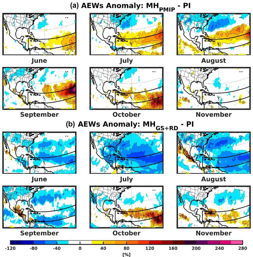
S. Dandoy et al.: Atlantic hurricane response during the MH                                                                    677

                                                                  sic representation of aerosol, accounting for only the extinc-
                                                                  tion coefficient, single scattering albedo and asymmetry fac-
                                                                  tor for continental and maritime particles. These values are
                                                                  spread evenly over the longitudes with higher values at the
                                                                  Equator and lower at the poles and higher values over land
                                                                  than over the ocean. Given such a coarse representation of
                                                                  the aerosol optical properties, we did not change them when
                                                                  performing the regional MHGS+RD experiment. Therefore,
                                                                  the major impacts of dust changes in the regional simulation
                                                                  (MHGS+RD ) were accounted for through the changes in the
                                                                  prescribed SST and lateral boundary conditions.

                                                                  2.3   Tracking algorithm

                                                                  In this study, a storm-tracking algorithm was developed using
                                                                  a three-step procedure (storm identification, storm tracking
                                                                  and storm lifetime) to detect tropical cyclones, following pre-
Figure 1. CRCM6 simulation domain (red box). The black/green      vious studies (Gualdi et al., 2008; Scoccimarro et al., 2011;
shaded box shows the approximate present-day tropical cyclone     Walsh et al., 2007). In comparison to most routines, our al-
main development region (MDR). Note that the data are projected   gorithm performs a double filtering approach similar to that
over an equidistant cylindrical projection.
                                                                  applied in Caron and Jones (2012) to ensure that the gene-
                                                                  sis and dissipation phases of TCs are well represented and
                                                                  that TCs are not counted twice in the case of a temporary
face Scheme (CLASS; Verseghy, 2000, 2009) and the FLake           decrease of intensity followed by a restrengthening. Looser
lake model (Mironov, 2008; Martynov et al., 2012) to repre-       detection criteria (with lower values than the standard thresh-
sent the different surfaces. More details regarding GEM4.8        olds values) were first used in order to detect all storm cen-
can be found in Girard et al. (2014). In this study, CRCM6        ters; then criteria were enforced to standard values following
is integrated on a domain encompassing the Atlantic Ocean         the literature (strict criteria). Centers that satisfy the strict
from Cabo Verde to the North American west coast (0 to            criteria are then classified as being “strong” centers (storm
45◦ N and ∼ 25 to 120◦ W; see Fig. 1).                            identification), while the others are classified as “weak” cen-
                                                                  ters. To correctly represent each track (storm tracking), the
2.2   Experimental design                                         strong and weak centers are then paired following two dif-
                                                                  ferent methods: the storm history using a similar approach
We performed three distinct 30-year experiments with              to that of Sinclair (1997) and the nearest-neighbor method
CRCM6 (see Table 1). The first experiment, the control or         as in Blender et al. (1997), Blender and Schubert (2000) and
reference case, is a pre-industrial (PI; performed at 0.11        Schubert et al. (1998). Once the storm tracks are defined, the
and 0.22◦ for validation purposes only) climate simulation        algorithm determines the core of each track as the centers
that follows the protocol set by the Paleoclimate Modelling       sitting between the first and the last strong centers found in
Intercomparison Project (PMIP) and the fifth phase of the         the track, thus neglecting the genesis and dissipation phases.
Coupled Model Intercomparison Project (CMIP5) (Taylor et          This subsection of the track (representing the main TC life-
al., 2012). Two MH simulations were also performed: in the        time) has to satisfy a third set of criteria that reject TCs that
first one, the PMIP protocol is followed, only accounting for     do not live long enough, that do not travel a long-enough dis-
changes in the orbital forcing (∼ 5 % increase in Northern        tance or that do not reach the strength of a tropical storm. If
Hemisphere insolation compared to present-day values) and         the core of the storm track satisfies all these criteria, the gen-
the greenhouse gas concentrations (MHPMIP ) relative to PI.       esis and dissipation phases (represented by the weak centers
The aim here is to evaluate the effect of the insolation forc-    that occurred before the first and after the last strong cen-
ing alone on TC activity compared to the reference case. In       ters) are added to form the complete storm track. A detailed
the second MH experiment, in addition to the changes in the       description of the storm identification and tracking can be
MHPMIP , the Sahara (11–33◦ N, 15◦ W–35◦ E) was replaced          found in Appendix A.
by evergreen shrub and airborne dust concentrations reduced
by up to 80 % in the EC-Earth experiment (MHGS+RD ) rela-         2.4   Potential intensity and genesis indices
tive to PI. Due to those changes in vegetation in the Sahara,
the albedo of the region decreased from 0.30 to 0.15 and the      Many environmental proxies have been used to link the
leaf area index increased from 0.2 to 2.6 (for details refer to   changes in the dynamical and thermodynamical fields to TC
Pausata et al., 2016, and Gaetani et al., 2017). GEM has a ba-    activity. Here, two well-known environmental proxies were

https://doi.org/10.5194/cp-17-675-2021                                                           Clim. Past, 17, 675–701, 2021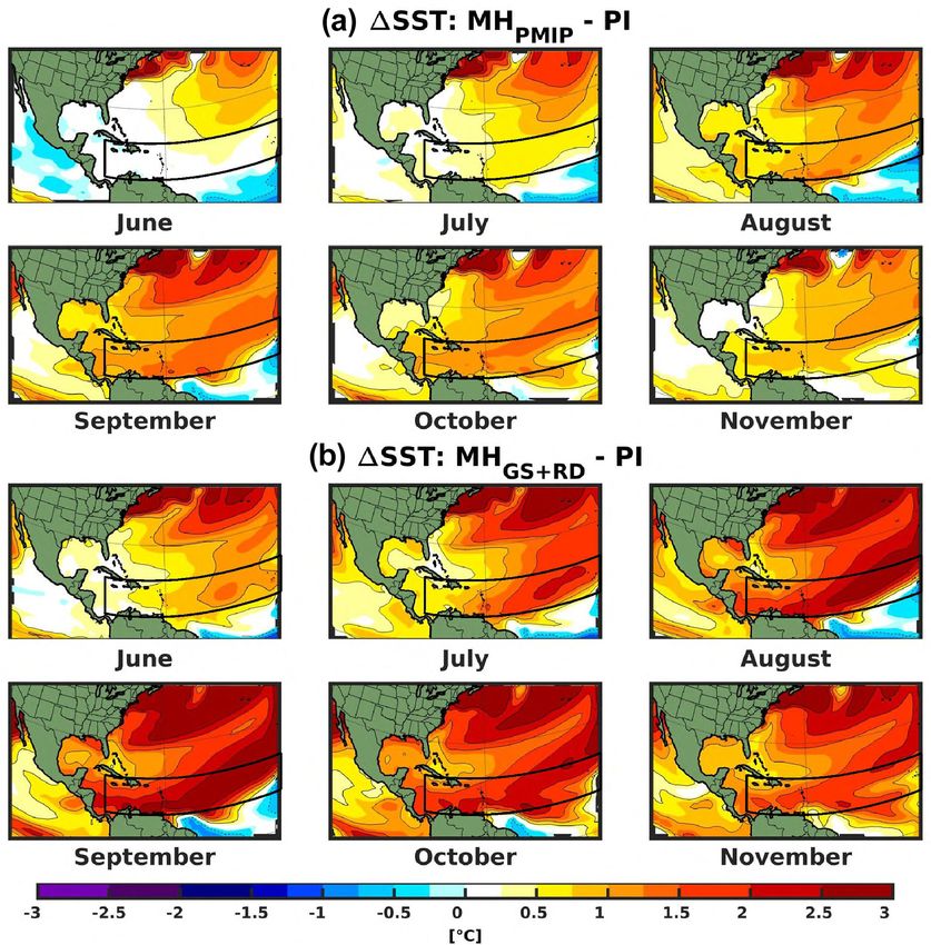
678                                                                S. Dandoy et al.: Atlantic hurricane response during the MH

Table 1. Boundary conditions for each modeling experiment.

                                Simulation   Orbital           GHGs             Saharan      Saharan
                                             forcing                            vegetation   dust
                                PI           1950              1850             Desert       PI
                                MHPMIP       6000 years BP     6000 years BP    As PI        As PI
                                MHGS+RD      6000 years BP     6000 years BP    Shrub        Reduced

adopted – the potential intensity (VPI ) and the genesis po-          (600 hPa) and the saturation entropy at the sea surface. Other
tential index (GPI) – to investigate the changes between dif-         indices have shown similar performance to the GPI, as, for
ferent climate states in TC achievable intensity and in the           example, the tropical cyclone genesis index (TCGI; Tippett
areas more prone to develop TCs, respectively. To calcu-              et al., 2011; Menkes et al., 2011).
late the theoretical maximum intensity of TCs given spe-
cific environmental conditions, the VPI formulation includes
the SST, the temperature at the level of convective outflow           2.5   Regional model evaluation
(To ), the ratio of drag and enthalpy exchange coefficients
(Ck /Cd = 0.9) and the available potential convective energy          To evaluate the CRCM6 performance in simulating tropical
difference between an air parcel lifted from saturation at            cyclones, an additional 0.22◦ simulation was carried out us-
sea level (CAPE∗ ) at the radius of maximum winds and an              ing the ERA-Interim reanalysis as lateral boundary condi-
air parcel located in the boundary layer (CAPEb ). The for-           tions and SSTs, and compared with 25 km ERA5 reanalysis
mula defined by Emanuel (1995) and updated by Bister and              data for the period 1980 to 2009 (see Hersbach et al., 2018).
Emanuel (1998, 2002) was used to account for dissipative              Our storm-tracking algorithm was used to detect tropical
heating:                                                              cyclones in the ERA5 reanalysis for validation and to en-
                                                                      sure the accuracy of simulated results against the observed
                                                                      track density obtained from the Atlantic “best-track” dataset
        s
          Ck · SST
                    CAPE∗ − CAPEb .

VPI =                                                     (1)         (the revised Atlantic hurricane database; HURDAT2) (Land-
           Cd · To                                                    sea and Franklin, 2013) for the same period (1980–2009).
                                                                      The use of the high-resolution ERA5 reanalysis data allowed
The GPI is an empirical fit of the most important environ-
                                                                      us to directly compare the obtained results to our modeled
mental variables known to affect TC formation. These vari-
                                                                      0.22◦ data and the HURDAT2 observations. The compari-
ables include dynamical (wind shear and absolute vorticity)
                                                                      son between the detected TCs in ERA5 reanalysis data and
and thermodynamical (potential intensity and moist entropy
                                                                      the observed TCs from the HURDAT2 database also pro-
deficit) factors. The first genesis index was introduced by
                                                                      vided a quick test case to evaluate ERA5 ability to repre-
Gray (1975, 1979). Since then, various genesis indices have
                                                                      sent observed TCs while using the same detection criteria,
been formulated (e.g., Emanuel and Nolan, 2004; Emanuel,
                                                                      which cannot be done with the coarser resolution of the raw
2010; Korty et al., 2012). Here, the genesis index formula-
                                                                      ERA-Interim data (∼ 80 km). The model evaluation is pre-
tion from Korty et al. (2012) was used, which is a modified
                                                                      sented in Appendix A. In general, our tracking algorithm
version of the GPI described in Emanuel (2010). This GPI in-
                                                                      captures well the main characteristics of the observed tracks
cludes the entropy deficit between different atmospheric lev-
                                                                      (Fig. A1). However, the number of detected TCs in ERA5
els, as the one of Emanuel (2010), with the addition of the
                                                                      data is lower than observations, even when considering lower
“clipped vorticity” (Tippett et al., 2011):
                                                                      threshold values. On the other hand, when comparing the
                            3                                       ERA-Interim-driven model-simulated TCs in the simulation
        a min |η| , 4 × 10⁻⁵ [max (VPI − 35, 0)]2

GPI =                                                  ,     (2)      against observations, there is a better agreement in the mean
                     χ 4/3 [25 + Vshear ]4                            track characteristics and number of Atlantic TCs (Fig. A1a).
                                                                      Murakami (2014) and Hodges et al. (2017) found signifi-
where VPI is the potential intensity, Vshear is the wind shear
                                                                      cant biases in the representation of TCs in various reanalysis
between 250 and 850 hPa levels, η is the absolute vorticity
                                                                      datasets, using different tracking algorithms. Although these
at 850 hPa, and a is a normalization coefficient. The entropy
                                                                      results strongly stem from the tracking algorithm’s ability to
deficit χ is defined as
                                                                      capture weaker storms, our comparison between the HUR-
      sb − sm                                                         DAT2 TC tracks and those obtained with ERA5 reanalysis
χ=             ,                                             (3)      shows important differences between the two.
      so∗ − sb
                                                                         In this study, we use a two-tailed Student t test to deter-
where sb , sm and so∗ represent, respectively, the moist en-          mine the statistical significance of changes at the 5 % confi-
tropies of the boundary layer (900 hPa), middle troposphere           dence level. The significance of the changes in TC frequency

Clim. Past, 17, 675–701, 2021                                                            https://doi.org/10.5194/cp-17-675-2021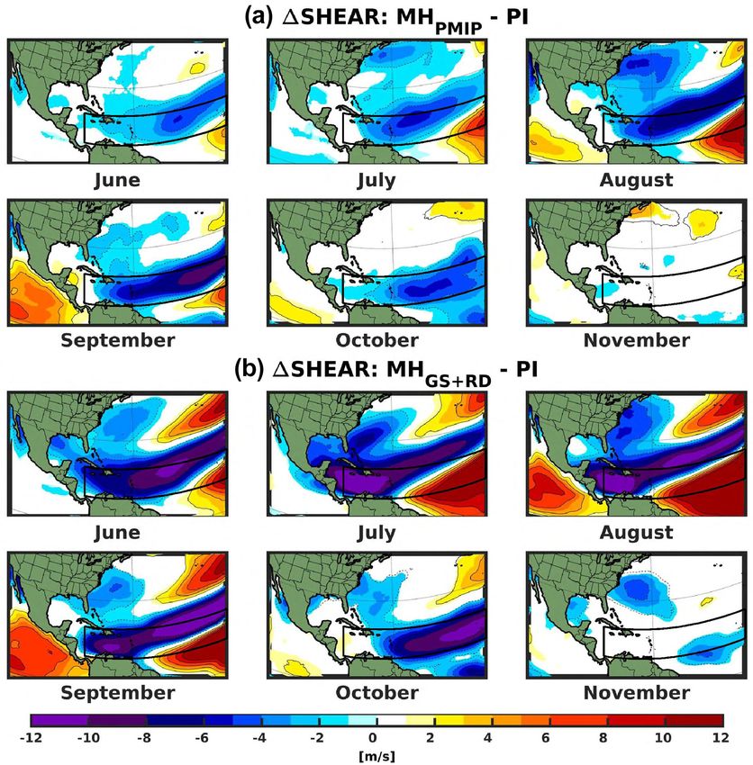
S. Dandoy et al.: Atlantic hurricane response during the MH                                                                  679

has been determined using twice the standard error of the           et al., 2014; Seth et al., 2019). The ITCZ is associated with
mean (∼ 5 % confidence level). The accumulated cyclone en-          more favorable conditions for cyclogenesis by increasing the
ergy (ACE; Bell et al., 2000) was also calculated. ACE is           ambient vorticity and therefore the TC activity (Merlis et
defined as the sum of the square of the maximum sustained           al., 2013). Our analysis shows that the absolute vorticity
wind speed (in knots; 1 kn = 0.514 m s−1 ) higher than 35 kn        maximum undergoes a northward shift relative to the control
every 6 h over all the storm tracks. ACE is an integrated mea-      experiment, following the ITCZ displacement (Fig. A5), sup-
sure depending on TC number, intensity and duration, and            porting the northward shift of the TC tracks (Fig. 2c). Higher
less sensitive than TC counts to tracking schemes and thresh-       absolute vorticity values are also found over the Greater An-
olds (Zarzycki and Ullrich, 2017). Besides the total ACE, the       tilles and the western part of the Gulf of Mexico where there
mean ACE per storm was also considered, and ACE per mean            is a higher TC occurrence in the MHGS+RD relative to PI.
storm duration, in order to analyze the contribution of the dif-        The northward shift and the increase of TC activity in
ferent components of ACE to the total value.                        the MH experiments are also related to the strengthening of
   To evaluate the statistical significance in the difference       the WAM, which amplifies the westerly winds, and the SST
in TC counts between different climate states, a bootstrap          anomaly (Fig. A6). Such changes lead to the development of
method was used to create 100 randomly selected 30-year             a wind shear pattern anomaly in the MDR, with lower val-
samples out of the 40-year (1979–2018) distributions of the         ues of wind shear in the central–western region of the MDR
annual number of observed TCs and ERA5 TCs.                         and higher values on the eastern side of the MDR relative
                                                                    to PI. Thus, while the area more favorable for TC devel-
3     Results                                                       opment is reduced (Fig. A7), the more favorable conditions
                                                                    present on the western side more than compensate the de-
In this section, the TCs in the MH and PI climate conditions        crease in the east, allowing more cyclones to develop in the
are studied to evaluate how changes in orbital forcing, dust        MH experiment. In addition to the zonal atmospheric circu-
and vegetation feedbacks impact TC activity in the Atlantic         lation changes, the enhanced northward penetration of the
Ocean, by focusing on TC trajectories and annual frequency          WAM together with the displacement of the ITCZ leads to a
(Sect. 3.1), seasonality (Sect. 3.2) and intensity (Sect. 3.3).     northward shift of the maximum in AEW activity in the MH
We also highlight the impacts of such changes on the differ-        experiments relative to PI (see Fig. A8). The poleward dis-
ent variables known to affect TC genesis.                           placement of the AEWs may also contribute to the changes
                                                                    in TC genesis location as they influence the region where
                                                                    TCs develop (e.g., Caron and Jones, 2012).
3.1    Change in TC density and frequency
                                                                        The vegetation changes and the associated reduction in
The PI climate simulation has a spatial distribution of At-         dust concentrations further strengthen the WAM in the
lantic hurricanes that is similar to present climate, where         MHGS+RD relative to the MHPMIP experiment (Pausata et
most of the TCs form in the main development region (MDR)           al., 2016, 2017), hence amplifying the changes seen in
and move west–northwestward towards the North American              the MHPMIP . Furthermore, the reduction in dust concentra-
east coast (Fig. 2b). However, there are fewer TCs in the sim-      tion in the MHGS+RD experiment directly affects the SST
ulated PI climate than in the present-day climate simulation        (Fig. A6b), leading to an environment more prone to de-
driven by ERA-Interim (cf. Fig. 2a and A2); this is due to          velop TCs relative to the MHPMIP and PI simulations. This
a large extent to the SST cold bias in the EC-Earth simula-         is consistent with previous studies that found that the Saha-
tion (∼ 5 ◦ C; see Fig. A3). When only the orbital forcing is       ran dust layer can have large impacts on TC activity (Evan et
considered (MHPMIP ), there is a northward shift of the At-         al., 2016; Pausata et al., 2017; Reed et al., 2019).
lantic TC tracks, as well as an eastward displacement of the            The GPI anomalies of both MH experiments relative to PI
tracks away from the US east coast at higher latitudes and a        closely follow the changes in the atmospheric and oceanic
small increase in the TC track density relative to the PI ex-       environmental factors that can affect TCs (cf. Figs. 3, A5–
periment (Fig. 2c). This anomaly pattern is similar to that         A9). The GPI shows more favorable conditions with higher
of the MHGS+RD experiment, but the anomalies are notably            values of vorticity and SST and lower wind shear values.
stronger in the latter simulation (Fig. 2d), extending further      Similarly to the absolute vorticity field (Fig. A5), the GPI
north and westward into the Greater Antilles and Gulf of            shows a small northward shift relative to the control experi-
Mexico. The TC northward shift in the MH experiments and            ment, thus contributing to the poleward displacement of the
the strong eastward shift at higher latitudes are related to both   TC genesis locations and therefore the the TC tracks (cf.
the northward displacement of the ITCZ and the intensifica-         Figs. 3 and 4).
tion of the WAM relative to the PI simulation (Fig. A4).                The largest changes in GPI are seen in the MHGS+RD ex-
   The northward shift of the ITCZ in the MH is due to ener-        periment (Fig. 3b). The greening of the Sahara and the re-
getic constraints associated with the changes in orbital forc-      duced dust concentrations over the Atlantic Ocean not only
ing causing a warming of the NH and a cooling of SH during          lead to higher potential for cyclogenesis in the MDR but also
boreal summer relative to PI (Merlis et al., 2013; Schneider        extend the region westward towards the Caribbean where the

https://doi.org/10.5194/cp-17-675-2021                                                           Clim. Past, 17, 675–701, 2021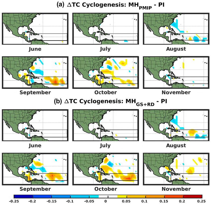
680                                                                     S. Dandoy et al.: Atlantic hurricane response during the MH

Figure 2. June to November (JJASON) climatology of (a) track density for the pre-industrial (PI) experiment; (b) TC frequency in the
Atlantic Ocean for each experiment. Error bars (whiskers) indicate the standard error of the mean; changes in track density for the MHPMIP (c)
and the MHGS+RD (d) experiments relative to the PI. The black box shows the present-day MDR; the dotted red box shows the approximate
shift of the MDR in the MH experiments. Only values that are significantly different at the 5 % level using a local (grid-point) t test are
shaded. The contour lines follow the color-bar scale (dashed, negative anomalies; solid, positive anomalies); the 0 line is omitted for clarity.

Figure 3. Changes in seasonal GPI (JJASON) for (a) MHPMIP and (b) MHGS+RD experiments relative to PI. The black box shows the
approximate present-day MDR. Only values that are significantly different at the 5 % level using a local (grid-point) t test are shaded. The
contour lines follow the color-bar scale (dashed, negative anomalies; solid, positive anomalies); the 0 line is omitted for clarity.

model simulates a higher occurrence of TCs in this experi-                lies relative to PI present a net northward displacement of its
ment relative to the PI (see Fig. 2c). Overall, the changes in            locations, highlighting an important difference between the
cyclogenesis density for both MH experiment follow closely                two downscaling techniques (see Fig. A10). These changes
the changes in GPI (cf. Figs. 3 and 4), suggesting that GPI               in the TC genesis are likely responsible for the downstream
is a good predictor of the TC activity changes, even in very              changes in the TCs’ track density in both studies.
different climate states. Moreover, in Pausata et al. (2017),                In terms of frequency, an average of 5.5 TCs per year is
the TC genesis anomalies in the MH experiments show a                     simulated in the PI experiment (Fig. 2b). This is ∼ 45 %
westward shift, while in our analysis the TC genesis anoma-               less than the present-day climatology (∼ 10 TCs per year;

Clim. Past, 17, 675–701, 2021                                                                    https://doi.org/10.5194/cp-17-675-2021
S. Dandoy et al.: Atlantic hurricane response during the MH                                                                      681

Figure 4. TC seasonal (JJASON) cyclogenesis density anomaly for (a) MHPMIP and (b) MHGS+RD experiments relative to PI represented
over a 5◦ mesh-grid Mercator projection. The black box shows the approximate present-day MDR.

Landsea, 2014), which is likely due to a strong cold bias in
the SST of the coupled model simulation (see Fig. A3 and
Pausata et al., 2017). Many high-resolution global models
have similar biases in the Atlantic (e.g., Shaevitz et al., 2014;
Wing et al., 2019). The MHPMIP experiment shows a small
increase (+9 %; statistically significant) in the TC frequency
relative to the PI, highlighting the minor impact of the or-
bital forcing alone on the number of Atlantic TCs (Fig. 2b).
In the MHGS+RD simulation, more TCs are generated (7 per
year) with a significant increase of around 1.5 TCs per year
(+27 %) relative to the PI experiment (Fig. 2b). Bootstrap
tests with both HURDAT2 (Fig. 5a) and ERA5 (Fig. 5b)
datasets show that the chances of obtaining an increase of
27 % (9 %) in the mean of each distribution are signifi-
cantly (slightly) higher than the 95th percentile of these dis-
tributions. Our sensitivity experiments hence roughly show
that the orbital forcing alone contributes for about 33 % (∼
0.5 TCs per year) of the total increase in TC frequency occur-
ring in the MHGS+RD relative to the PI experiment, while the
Saharan greening and reduced dust concentrations account
for about 66 % of this increase (∼ 1 TC per year). Thus,
these results suggest that the TC activity is strongly domi-
nated by the vegetation and dust changes, in close agreement
with Pausata et al. (2017).

                                                                    Figure 5. Bootstrap distributions based on (a) the 1979–2018
3.2   Changes in TC seasonal cycle                                  HURDAT database and (b) 1979–2018 ERA5 reanalysis data. The
                                                                    legend presents the median, mean, standard deviation, 5th and 95th
To analyze changes in TC seasonal cycle, we consider                percentiles of the distributions.
changes in the monthly number of TCs rather than change
of the length of the TC season. The PI climate has a TC sea-
sonal cycle that is similar to the present climate, with a peak        Gaetani et al. (2017), using the same global model experi-
in TC in September (Fig. 6). The MH experiments show a              ments performed with EC-Earth, showed a large decrease in
distinct pattern: a decrease in TC activity at the beginning        the AEWs in the MHGS+RD relative to the MHPMIP simula-
of the hurricane season for both MH experiments (statisti-          tion due to the strengthening of the WAM. As AEWs can
cally significant for the MHPMIP in July and August; non-           potentially act as seeds for TC genesis (Caron and Jones,
significant for the MHGS+RD ), followed by a large increase at      2012; Frank and Roundy, 2006; Landsea, 1993; Thorncroft
the end of TC season (statistically significant during Septem-      and Hodges, 2001), we analyze the changes in the AEW sea-
ber and October in the MHPMIP ; MHGS+RD from September              sonality in the MH experiments relative to PI to determine
to November, SON) relative to PI.                                   whether there is a direct link between the changes in the sea-

https://doi.org/10.5194/cp-17-675-2021                                                             Clim. Past, 17, 675–701, 2021
682                                                                S. Dandoy et al.: Atlantic hurricane response during the MH

                                                                    tion) and the frequency of disturbances determined the TC
                                                                    frequency in their model.
                                                                       Other factors could be playing a role in modifying the TC
                                                                    seasonal cycle. In particular, the shift in TC seasonal cycle
                                                                    could be related to changes in the orbital forcing, most im-
                                                                    portantly the precession of the equinoxes: during the MH,
                                                                    the perihelion was in September instead of January, as to-
                                                                    day, with the stronger insolation anomalies peaking in late
                                                                    summer at NH low latitudes. Furthermore, while higher po-
                                                                    tential intensity (due mostly to warmer SSTs; see Figs. A6
                                                                    and A11) develops on the western part of the MDR and most
                                                                    of the North Atlantic Ocean from June to September relative
                                                                    to the PI experiment, the strengthening of the WAM causes
                                                                    a cold anomaly response over the eastern part of the MDR,
Figure 6. TC climatological distribution throughout the extended    together with stronger vertical wind shear and weaker ab-
TC season (JJASON) for each experiment. Error bars (whiskers)       solute vorticity values. The withdrawal of the WAM in late
indicate the standard error of the mean.                            September then causes the decrease in wind shear and posi-
                                                                    tive anomalies in both absolute vorticity and SSTs to extend
                                                                    eastward. These environmental anomalies are likely the rea-
                                                                    son for the TC seasonality changes during the MH experi-
sonality of AEW and TCs (Fig. 7). The AEWs’ activity is             ments (Figs. A11a, A12a, A13a). The cyclogenesis anoma-
remarkably reduced between July and September – 80 % less           lies and the GPI changes are consistent with these assump-
relative to PI – and intensified in October and November in         tions (cf. Figs. 9a and A14a). Korty et al. (2012), who studied
the MHGS+RD relative to PI (Fig. 7b).                               the response to orbital forcing in PMIP2 models during the
   The reduction of the AEWs in the MHGS+RD experiment              MH, also found that the TC season in the Northern Hemi-
is related to the strengthening and northward shift of the          sphere was less favorable during summer, while it became
WAM. The anomalous westerly wind flow associated with               more favorable during fall (October and November) relative
the northward expansion of the WAM rainfall significantly           to pre-industrial climate. The authors pointed out that these
alters the African easterly jet (AEJ) (Fig. 8) and the Saharan      findings were due to the difference between the warming rate
heat low. In particular, the disappearance of the 600 hPa AEJ       of the atmosphere (which warms faster during the summer
and northward displacement of the wind circulation are re-          months) and that of the ocean surface, which led to a nega-
sponsible for the lower frequency of AEWs during the sum-           tive potential intensity anomaly during the first half of their
mer months in the MHGS+RD relative to PI. On the other              TC season (June to September) and a positive anomaly dur-
hand, the withdrawal phase of the WAM towards the end of            ing the second half (October to November). Using PMIP3
the season (SON) is associated with an increase in the fre-         models, Koh and Brierley (2015) drew similar conclusions;
quency of AEWs relative to PI, potentially contributing to the      however, the changes in fall were not a robust signal across
increase in TC activity in those months. While the changes          models.
in the frequency of AEWs in the MHGS+RD are potentially in             Accounting for the Saharan greening and reduced airborne
agreement with the simulated changes in TC seasonality, the         dust concentrations (MHGS+RD ) leads to even larger changes
frequency of AEWs in the MHPMIP is higher relative to PI,           relative to PI (Figs. A11b, A12b, A13b), strengthening the
especially in June and July, which is at odds with the changes      GPI anomalies in the MDR (Fig. 9b). These changes strongly
in TC frequency in the MHPMIP experiment (no change in              increased the total GPI over the ocean from September to
June and slight decrease in July; Fig. 7a). Furthermore, in         November in the MHGS+RD experiment and led to almost
July and August, fewer TCs are simulated in the MHPMIP              twice as many cyclones in November relative to the PI and
relative to the MHGS+RD , which has fewer AEWs. Hence,              MHPMIP experiments (see Figs. 6, 10 and A14b). Further-
it is not possible to draw a direct link between the changes        more, there is a westward extension of the region prone to TC
in the seasonality of AEWs and TCs between the MH and               development towards the Greater Antilles and the Caribbean
the PI simulations. These results agree with the findings of        Sea from July to September relative to the other two exper-
Patricola et al. (2018) that, while AEWs can affect TC gen-         iments (Figs. 9b and 11), which is also reflected in the sea-
esis, their contribution may not be necessary, and TCs can          sonal GPI (Fig. 3b). These anomalies led to a small increase
also be formed from other processes such as wave breaking           in cyclogenesis over the Caribbean Sea relative to PI during
of the ITCZ, disturbance from the Asian monsoon trough or           this part of the season and may explain the increased TC ac-
self-aggregation of convection (Patricola et al., 2018). Fur-       tivity during July and August in the MHGS+RD relative to the
thermore, Vecchi et al. (2019) showed that a combination of         MHPMIP and why almost as many cyclones formed during
the large-scale environmental factors (in particular ventila-       September (cf. Figs. 6, A14).

Clim. Past, 17, 675–701, 2021                                                           https://doi.org/10.5194/cp-17-675-2021
S. Dandoy et al.: Atlantic hurricane response during the MH                                                                                  683

Figure 7. Monthly AEW anomalies represented through the variance of the meridional wind at 700 hPa, filtered in the 2.5 to 5 d band, for
(a) MHPMIP and (b) MHGS+RD relative to PI. The black box shows the approximate present-day MDR. Only values that are significantly
different at the 5 % level using a local (grid-point) t test are shaded. The contour lines follow the color-bar scale (dashed, negative anomalies;
solid, positive anomalies); the 0 line is omitted for clarity.

Figure 8. AEJ represented through a vertical cross section of zonal mean (0–40◦ N; 20–30◦ W) seasonal climatological zonal winds for
(a) PI and (b) MHGS+RD experiments, respectively.

https://doi.org/10.5194/cp-17-675-2021                                                                       Clim. Past, 17, 675–701, 2021
684 S. Dandoy et al.: Atlantic hurricane response during the MH
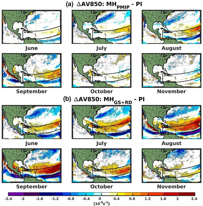
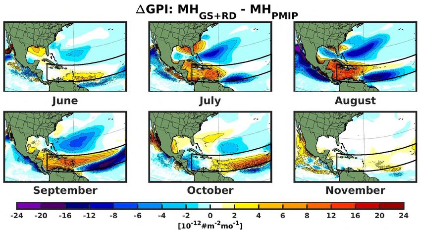
Figure 9. Changes in climatological monthly GPI for (a) MHPMIP and (b) MHGS+RD relative to the PI experiment. The black box shows
the approximate present-day MDR. Only values that are significantly different at the 5 % level using a local (grid-point) t test are shaded.
The contour lines follow the color-bar scale (dashed, negative anomalies; solid, positive anomalies); the 0 line is omitted for clarity.
3.3 Changes in intensity simulations arises from two different aspects: (1) TCs in the
MH climate are more intense than in the PI experiment (as
To assess TC intensity, we considered the 10 m maximum shown in Fig. 12), therefore leading to higher rate of energy
wind speed in 3 h intervals and then classified them using generation, and (2) TCs in the MH experiments tend to last
the Saffir–Simpson scale categories. For the three experi- longer (PI: 199 h, MHPMIP : 217 h and MHGS+RD : 283 h; see
ments, most tropical cyclones reach only tropical storm or legend in Fig. 13c), meaning that the same amount of energy
hurricane Category 1 (93 %, 88 % and 91 % for PI, MHPMIP can be spend over a longer time lapse. The combination of
and MHGS+RD , respectively), with only a few reaching Cat- these two aspects with increased mean TC count per season
egory 2 (7 %, 11 % and 8 %) (Fig. 12). Both MH simulations in the MH experiments (Figs. 2b and 14a) therefore leads to a
generated Category 3 hurricanes (∼ 1 % in both cases), while larger total mean ACE per experiment in the MH simulations
there were no major hurricanes in the PI experiment. Our compared to PI (see legend in Fig. 13b).
analysis of the ACE also reveals that, in general, the mean To better understand the cause of these changes, we turn
ACE per cyclone in the MH experiments is higher than in the to the seasonal VPI (Fig. 14) and examine the regions where
PI experiment (∼ 6.6 × 10⁴ m2 s−2 and ∼ 7.4 × 10⁴ m2 s−2 the atmospheric conditions are more favorable for TC in-
for MHPMIP and MHGS+RD , respectively, ∼ 6.1×10⁴ m2 s−2 tensification. The area showing the most favorable condi-
for PI; see legend in Fig. 13c). The increase in ACE in MH
Clim. Past, 17, 675–701, 2021 https://doi.org/10.5194/cp-17-675-2021S. Dandoy et al.: Atlantic hurricane response during the MH 685
BP). We compared two different MH experiments – where
only orbital forcing is considered (MHPMIP ) and where also
changes in vegetation and dust concentration are accounted
for (MHGS+RD ) – to a control PI experiment. Our results
show that the Saharan greening and related reduction in
dust concentrations (MHGS+RD experiment) significantly in-
crease the number of TCs in the North Atlantic Ocean by
about 27 %, whereas the increase associated with the or-
bital forcing alone is smaller (9 %; MHPMIP ). In general,
our results are consistent with the findings of Pausata et
al. (2017), who used the same coupled global model sim-
ulation to drive a statistical–thermodynamical downscaling
Figure 10. Seasonal variation (JJASON) of the GPI summed over technique (Emanuel et al., 2008) to assess changes in TC ac-
the experimental domain for the three experiments. tivity; however, the changes in TC activity simulated in our
study between the MH experiments and the PI simulation are
smaller. Furthermore, the displacement of TC activity is dif-
tions for cyclone intensification in the MHPMIP relative to ferent in our study (meridional vs. zonal) and most likely re-
the PI experiment is located around the central–western por- lated to the fact that dynamical changes in ITCZ and AEW
tion of MDR and extends northwards over the central At- are not accounted for in Pausata et al. (2017). Our experi-
lantic Ocean and westward along the northernmost part of ments show that the MH climate induces a northward shift of
the US east coast (Fig. 14a). Less favorable conditions are the North Atlantic TC tracks and an eastward displacement
present east and south of the MDR where colder SSTs are of those away from the US east coast at higher latitudes. A
present. The mean VPI pattern for the MHGS+RD yields even zonal shift of the storm track relative to PI is instead sim-
stronger anomalies than the ones simulated by the MHPMIP , ulated in Pausata et al. (2017). Our work also suggests an
with substantially more favorable conditions for intensifica- important reduction of the TC activity during the first half of
tion in the MDR (Fig. 14b). More conducive conditions are the TC seasonal cycle in the MH experiments together with
also present in the Caribbean Sea, where markedly lower val- a shift of the maximum TC activity towards the second half.
ues of vertical wind shear are simulated (Fig. A7). The com- Gaetani et al. (2017) showed a strong decrease in AEW in
bination of more favorable environmental conditions (e.g., the MHGS+RD simulations and suggested a potential impact
wind shear) along with the occurrence of more TCs cross- on TC activity; however, our analysis does not show a consis-
ing this area in the MHGS+RD experiment relative to both tent relationship between the frequency of AEWs and tropi-
PI and MHPMIP (see Fig. 2d) increases the chances of get- cal cyclones. These results support the findings of Patricola
ting more intense and long-living cyclones. The main fac- et al. (2018), who showed through a set of sensitivity experi-
tors contributing to the increase in VPI in the MHGS+RD rela- ments that the AEWs may not be necessary for TC genesis as
tive to the PI and MHPMIP experiments are the warmer SSTs TC formation occurs even in the absence of AEWs through
(∼ 1.5 ◦ C higher; Fig. A6b) and enhanced levels of convec- other mechanisms. This is supported by observational stud-
tive available potential energy (CAPE; Fig. A15) as direct ies that could not find a direct relation in the frequency of
consequences of the reduced dust emissions. In comparison AEWs and TCs (Russell et al., 2017). Instead, the AEWs
to the change seen in the MHPMIP relative to PI, less favor- seem to play a more important role in the location of TC
able conditions for intensification are simulated north of the genesis rather than the total TC frequency. Furthermore, the
MDR in the MHGS+RD (Fig. 14b). Overall, the VPI anoma- RCM domain size and location of the lateral boundary condi-
lies for both MH experiments strongly resemble those pre- tions impact the frequency of AEWs TCs inside the domain
sented in Pausata et al. (2017) and closely follow the changes (Caron and Jones, 2012; Landman et al., 2005).
in GPI, therefore leading to more intense and potentially Our study suggests that the different orbital parameters to-
longer-living cyclones where better conditions are available gether with the changes in the WAM intensity may have been
for cyclogenesis. the main causes of the changes in TC seasonality, offering
better conditions for cyclogenesis towards the end of the hur-
ricane season. WAM intensity affects the wind shear on the
4 Discussion and conclusions eastern side of the MDR. The WAM withdrawal towards the
end of the summer extended the more favorable conditions
In this study, we use the CRCM6 regional climate model from the central–western portion towards the eastern portion
with a high horizontal resolution (0.11◦ ) to better investi- of the MDR, causing an increase in TC activity during the
gate the role played by vegetation cover in the Sahara and second half of the season in the MH simulations. These re-
airborne dust on TC activity in the Atlantic Ocean during sults are consistent with the findings of Korty et al. (2012),
a warm climate period, the mid-Holocene (MH, 6000 years who also showed higher cyclogenesis potential towards the
https://doi.org/10.5194/cp-17-675-2021 Clim. Past, 17, 675–701, 2021686 S. Dandoy et al.: Atlantic hurricane response during the MH
Figure 11. Changes in climatological monthly GPI for MHGS+RD relative to the MHPMIP experiment. The black box shows the approximate
present-day MDR. Only values that are significantly different at the 5 % level using a local (grid-point) t test are shaded. The contour lines
follow the color-bar scale with different styles (dashed, negative anomalies; solid, positive anomalies); the 0 line is omitted for clarity.
across different models and highlights an interesting point
where there may be a repression of the modeled environmen-
tal conditions that negatively affects proxies associated with
TC (i.e., the VPI and GPI) and supports these results during
the summer months, which is later offset by opposite changes
during the autumnal season in many of them. Moreover, even
if airborne dust variations are dominant in controlling the TC
annual total, the orbital forcing still has a detectable role in
affecting TC activity. Our work also shows that the GPI is
able to represent the regions more prone to TC development
in different climate states, in agreement with previous stud-
ies (Camargo et al., 2007; Koh and Brierley, 2015; Korty et
al., 2012; Pausata et al., 2017). The reduced dust emissions in
the MHGS+RD experiment induce an additional SST warm-
Figure 12. Climatological number of TCs per year in various cate- ing that enhances the available thermodynamic energy, in-
gories for the three experiment during the TC extended season (JJA- creasing the VPI even further compared to the MHPMIP and
SON). PI experiments and thus leading to more intense TCs. This
SST warming-induced effect is consistent with the model-
based projections for TC intensity in a warmer future cli-
mate (Knutson et al., 2013; Walsh et al., 2016; Knutson et
end of the PI hurricane season in their MH experiment, with al., 2020).
likely increase in TC activity during October when the GPI Finally, the simulated impact of dust changes needs fur-
is at its maximum. However, their results are based on the ther investigation, as rainfall in the north of Africa can be
entire Northern Hemisphere, while here we only focus on strongly affected by the dust optical properties (e.g., “heat
the North Atlantic Ocean. In addition, our results compare pump” effect where the atmospheric dust layer warms the
well to those of Koh and Brierly (2015), who found less fa- atmosphere, enhancing deep convection and intensifying the
vorable environmental conditions for TC development dur- WAM; see Lau et al., 2009). In particular, in EC-Earth, dust
ing Northern Hemisphere summer in the MH relative to pre- particles are moderately to highly absorbing particles (sin-
industrial when analyzing PMIP3 model simulations. Hence, gle scattering albedo ω0 < 0.95), with ω0 = 0.89 at 550 nm.
the impact on TCs on changes in orbital forcing is consistent
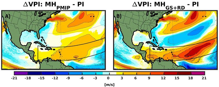
Clim. Past, 17, 675–701, 2021 https://doi.org/10.5194/cp-17-675-2021S. Dandoy et al.: Atlantic hurricane response during the MH 687 Figure 13. (a) Total number of cyclones per season for each experiment (30 years; gray: PI, yellow: MHPMIP and green: MHGS+RD ). (b) Total ACE (104 m2 s−2 ). (c) Mean ACE per cyclone per season (104 m2 s−2 ). (d) Mean ACE per cyclone normalized by the mean tropical cyclone duration in every season (104 m2 s−2 h−1 ). Legends present the climatological mean of each distribution. Figure 14. Changes in climatological seasonal VPI (JJASON) for the (a) MHPMIP and (b) MHGS+RD experiments relative to PI. The black box shows the present-day MDR. Only values that are significantly different at the 5 % level using a local (grid-point) t test are shaded. The contour lines follow the color-bar scale (dashed, negative anomalies; solid, positive anomalies); the 0 line is omitted for clarity. Such a value is too absorbing compared to observations (see etary albedo. This response is opposite to what one would Fig. 1 in Albani et al., 2014), and consequently the radia- expect from a reduced heat pump effect (decreased rainfall), tive impact of dust may well be overestimated. In a recent suggesting that the heat pump effect is overwhelmed by the study, Albani and Mahowald (2019) showed how different changes in surface albedo under green Sahara conditions in choices in terms of dust optical properties and size distribu- EC-Earth simulations. Another important aspect that was not tions may yield opposite results in terms of rainfall changes. considered in our study is dust–cloud interactions which may However, in the EC-Earth simulations, most of the changes further feed back in TC activity, both directly in the TC for- in the WAM intensity were associated with changes in sur- mation and indirectly by affecting the intensity of the WAM. face albedo due to greening of the Sahara, which was en- A recent study (Thompson et al., 2019) showed that this in- hanced by dust reduction through a further decrease in plan- teraction could indeed influence the WAM rainfall. There- https://doi.org/10.5194/cp-17-675-2021 Clim. Past, 17, 675–701, 2021
688                                                               S. Dandoy et al.: Atlantic hurricane response during the MH

fore, additional studies investigating the impact of dust opti-
cal properties and dust–cloud interactions on TC activity are
needed.
   In conclusion, our study highlights the importance of veg-
etation and dust changes in altering TC activity and calls
for additional modeling efforts to better assess their role
on climate. For example, employing regional model simu-
lations with atmosphere and ocean coupling will be impor-
tant to better represent the interactions between TC activ-
ity and TC–ocean feedbacks as a large amount of energy is
transferred through TC activity between the atmosphere and
the ocean (Scoccimarro et al., 2017). Furthermore, to val-
idate the model results, additional new paleotempestology
records across the Gulf of Mexico and Caribbean Sea will
be of paramount importance. While our study shows an in-
crease in TC frequency and intensity during a climate state
with warmer summers and a stronger WAM, it is difficult
to draw a direct conclusion for the future, as environmental
proxies associated with TCs (i.e., the VPI and GPI) are less
sensitive to temperature anomalies caused by CO2 than by
those caused by orbital forcing (Emanuel and Sobel, 2013).
However, in the view of a potential future “regreening” of the
Sahel and/or reduced Saharan dust layer, as shown in Biasutti
(2013), Evan et al. (2016) and Giannini and Kaplan (2019),
our work suggests that these changes may further enhance
TC frequency due to only greenhouse gases, in particularly
over the MDR, the Greater Antilles and the western portion
of the Gulf of Mexico, and could generate more intense and
potentially longer-living cyclones, increasing the vulnerabil-
ity of society to damages from severe TCs.

Clim. Past, 17, 675–701, 2021                                                         https://doi.org/10.5194/cp-17-675-2021
S. Dandoy et al.: Atlantic hurricane response during the MH                                                                 689

Appendix A: Tracking algorithm                                      b. minimum pressure difference between the center and a
                                                                       200 and 400 km radius greater than 4 and 6 hPa, respec-
In this study, we developed a tracking algorithm that makes            tively;
use of a three-step procedure to detect cyclones, follow-
ing previous studies (Gualdi et al., 2008; Scoccimarro et           c. relative vorticity maximum larger than 10−4 s−1 ;
al., 2011; Walsh et al., 2007).
                                                                   d. wind speed maximum above 17 m s−1 ; and
A1   Storm identification                                           e. warm core temperature anomaly above 2 ◦ C.
The storms are identified with the following criteria:            Another condition was added that only the strong centers
  a. The surface pressure at the center must be lower than        needed to satisfy:
     1013 hPa and lower than its surrounding grid boxes             f. The maximum wind velocity at 850 hPa must be larger
     within a radius of 24 km (21x); this pressure is then             than the maximum wind velocity at 300 hPa.
     taken as the center of the storm.
                                                                     In doing so, we avoided double counting cyclones that may
  b. The center must be a closed pressure center so that the      decreased in intensity before re-intensifying. Conditions (e)
     minimum pressure difference between the center and a         and (f) are the main conditions that filtered the TCs centers
     circle of grid points in a small and a large radius around   from other low-pressure systems and extratropical cyclones,
     the center (200 and 400 km radii) must be greater than       as TCs have a warm core in their upper part and stronger
     1 and 2 hPa, respectively.                                   low-level wind speed than other storms.
  c. There must be a maximum relative vorticity at 850 hPa
     around the center (200 km radius) higher than 10−5 s−1 .     A2   Storm tracking

 d. The maximum surface wind speed around the center              Storms were then tracked as follows: for each potential cen-
    (100 km radius) must be stronger than 8 m s−1 .               ter found, the algorithm used the nearest-neighbor method,
                                                                  which was also applied in many other studies (Blender et
  e. To account for the warm core, temperature anomalies          al., 1997; Blender and Schubert, 2000; Schubert et al., 1998),
     at 250, 500 and 700 hPa are calculated, where each           to find a corresponding center in the following 3 h time in-
     anomaly is defined as the deviation from a spatial mean      terval within a 250 km radius around the storm center. Once
     over a defined region. The sum of the temperature            two centers were paired, they formed a storm track. The po-
     anomalies between the three levels must then be larger       tential position of the next center to be a continuation of the
     than 0.5 ◦ C.                                                storm was then calculated using the storm history, based on
                                                                  the position of the previous two centers, which allowed us
  f. If there are two centers nearby, they must be at least       to establish a possible speed and direction for the predicted
     250 km apart from each other; otherwise, the stronger        center. A similar procedure was applied in Sinclair (1997)
     one is taken.                                                and was derived from Murray and Simmonds (1991). The al-
                                                                  gorithm then searches around the last storm center using the
To identify the genesis and dissipative phases of the TCs, a      nearest-neighbor method and around this potential position
double filtering approach was used, similar to that applied       at the next time step to find a matching center. The nearest
by Caron and Jones (2012). The aforementioned threshold           center was always chosen first.
values were used to first detect all the potential centers that
could belong to a storm for each time step. Then, these cri-
teria were enforced to the standard values (defined below)        A3   Storm lifetime
following the literature (Gualdi et al., 2008; Scoccimarro et     Once a track was completed, it had to satisfy the following
al., 2011; Walsh, 1997; Walsh et al., 2007), and these new        final conditions:
threshold values were applied to each center to identify the
ones that satisfied these enforced criteria among the poten-       1. The TC had to exist for at least 36 h (with a minimum
tial weak ones that were predefined. The centers that satisfied       of 12 centers at 3 h intervals).
the standard criteria were labeled by the algorithm as being
strong centers (or real TC centers), while those that only sat-    2. The TC needed to have at least 12 strong centers along
isfied the first set of criteria were identified as being weak        its entire track, so that the shortest TC had only strong
centers (with standard value properties defined below).               centers (36 h).
   The enforced criteria are the following:
                                                                   3. The TC had to travel at least 10◦ (∼ 1000 km) of com-
  a. surface pressure at the center deeper than 995 hPa;              bined longitude and latitude in its lifetime.

https://doi.org/10.5194/cp-17-675-2021                                                         Clim. Past, 17, 675–701, 2021
690 S. Dandoy et al.: Atlantic hurricane response during the MH
4. The number of strong storm centers needed to represent
at least 77 % of a subpart of the complete storm track
delimited by the first and last strong center found by
the algorithm. This way, we ensured that the storm was
classified as a TC during most of its time.
Figure A1. JJASON climatology (1980–2009) of (a) track density for the CRCM6 ERA-Interim-driven experiment at 0.22◦ ; (b) ERA5
reanalysis data at 0.25 ◦ ; (c) observed TCs from the HURDAT database at 0.11◦ and (d) ERA5 reanalysis data using weaker detection
criteria at 0.25◦ . The black box shows the present-day MDR. Note that the ERA5 figures are projected over a Mercator grid while the other
two figures use the equidistant cylindrical projection. The contour lines follow the color-bar scale.
Figure A2. Climatological track density (JJASON) for the (a) pre-industrial experiment at 0.22◦ and (b) ERA-Interim-driven experiment at
0.22◦ . (c) Changes in track density between the two simulations. The black box shows the approximate present-day MDR. Only values that
are significantly different at the 5 % level using a local (grid-point) t test are shaded. The contour lines follow the color-bar scale (dashed,
negative anomalies; solid, positive anomalies); the 0 line is omitted for clarity.
Clim. Past, 17, 675–701, 2021 https://doi.org/10.5194/cp-17-675-2021You can also read