Growing topography due to contrasting rock types in a tectonically dead landscape - Earth Surface Dynamics
←
→
Page content transcription
If your browser does not render page correctly, please read the page content below
Earth Surf. Dynam., 9, 167–181, 2021
https://doi.org/10.5194/esurf-9-167-2021
© Author(s) 2021. This work is distributed under
the Creative Commons Attribution 4.0 License.

                   Growing topography due to contrasting rock
                      types in a tectonically dead landscape
                 Daniel Peifer1,2 , Cristina Persano1 , Martin D. Hurst1 , Paul Bishop1 , and Derek Fabel3
                1 School of Geographical and Earth Sciences, University of Glasgow, Glasgow, G12 8QQ, UK
                    2 CAPES    Foundation, Ministry of Education of Brazil, Brasília, DF 70040-020, Brazil
                     3 Scottish Universities Environmental Research Centre, East Kilbride, G75 0QF, UK

                                  Correspondence: Daniel Peifer (peiferdaniel@gmail.com)

                                    Received: 11 August 2020 – Discussion started: 25 August 2020
                           Revised: 18 January 2021 – Accepted: 2 February 2021 – Published: 9 March 2021

       Abstract. Many mountain ranges survive in a phase of erosional decay for millions of years following the ces-
       sation of tectonic activity. Landscape dynamics in these post-orogenic settings have long puzzled geologists due
       to the expectation that topographic relief should decline with time. Our understanding of how denudation rates,
       crustal dynamics, bedrock erodibility, climate, and mantle-driven processes interact to dictate the persistence of
       relief in the absence of ongoing tectonics is incomplete. Here we explore how lateral variations in rock type,
       ranging from resistant quartzites to less resistant schists and phyllites, and up to the least resistant gneisses and
       granitic rocks, have affected rates and patterns of denudation and topographic forms in a humid subtropical,
       high-relief post-orogenic landscape in Brazil where active tectonics ended hundreds of millions of years ago. We
       show that catchment-averaged denudation rates are negatively correlated with mean values of topographic relief,
       channel steepness and modern precipitation rates. Denudation instead correlates with inferred bedrock strength,
       with resistant rocks denuding more slowly relative to more erodible rock units, and the efficiency of fluvial ero-
       sion varies primarily due to these bedrock differences. Variations in erodibility continue to drive contrasts in
       rates of denudation in a tectonically inactive landscape evolving for hundreds of millions of years, suggesting
       that equilibrium is not a natural attractor state and that relief continues to grow through time. Over the long
       timescales of post-orogenic development, exposure at the surface of rock types with differential erodibility can
       become a dominant control on landscape dynamics by producing spatial variations in geomorphic processes and
       rates, promoting the survival of relief and determining spatial differences in erosional response timescales long
       after cessation of mountain building.

1   Introduction                                                    isostasy are central mechanisms controlling the extended
                                                                    longevity of post-orogenic landforms (Gilchrist and Sum-
The question of how landscapes evolve in the aftermath of           merfield, 1990; Bishop and Brown, 1992; Bishop, 2007).
mountain building has intrigued geomorphologists since the          However, a range of other factors and interactions play es-
early stages of the discipline, and classic concepts such as        sential roles in the post-orogenic evolution of ancient land-
the cycle of erosion (Davis, 1899) and dynamic equilib-             scapes, including variations in bedrock incision dynamics
rium landforms (Hack, 1960) were defined in the context             (e.g. Baldwin et al., 2003; Egholm et al., 2013), mantle flow
of these post-orogenic landscapes (Bishop, 2007). In partic-        dynamics and their influence on the overlying crust (e.g.
ular, reasons for the persistence of high topographic relief        Gallen et al., 2013; Liu, 2014), vertical and lateral varia-
in ancient mountain belts for many millions of years after          tions in bedrock erodibility (e.g. Twidale, 1976; Bishop and
crustal thickening remain enigmatic. We know with a reason-         Goldrick, 2010; Gallen, 2018; Bernard et al., 2019; Vascon-
able degree of certainty that net erosion in these landscapes       celos et al., 2019), densification of the lower crust and result-
and the resulting rebound of the underlying lithosphere by

Published by Copernicus Publications on behalf of the European Geosciences Union.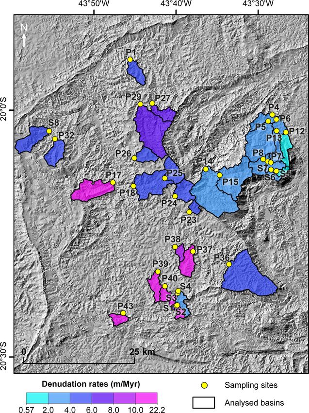
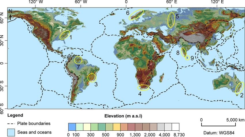
168                      D. Peifer et al.: Growing topography due to contrasting rock types in a tectonically dead landscape

ing reduction of the buoyancy of the lithosphere (e.g. Black-       dervan et al., 2020a). In particular, correlations between
burn et al., 2018), and tectonic uplift in response to far-field    rock type and topographic forms were observed in post-
stresses (e.g. Hack, 1982; Quigley et al., 2007).                   orogenic landscapes, with high topographic relief and steep
   Examples of ancient mountain belts marked by high el-            channel reaches associated with resistant rocks (e.g. Hack,
evations and steep slopes include the Appalachian Moun-             1960, 1975; Twidale, 1976; Mills, 2003; Spotila et al., 2015;
tains, several mountain ranges in southeastern Brazil, the          Gallen, 2018). These observations were interpreted, in sev-
Cape Mountains, parts of the East Australian Highlands,             eral cases, as equilibrium adjustments where spatial varia-
the Ural Mountains, the Caledonides, the Western Ghats,             tions in rock strength are balanced by variations in topo-
and the Sri Lanka orogen (Fig. 1). These high-relief post-          graphic relief so that everywhere is eroding at the same
orogenic settings are associated with different climate con-        rate, with the corollary that topographic forms are constant
ditions, tectonic histories, effective elastic thicknesses of the   through time in a “topographic equilibrium” likely driven
lithosphere, and geological architectures. For instance, some       by isostatic uplift (e.g. Hack, 1960; Matmon et al., 2003;
of these ancient mountain belts are located in a passive mar-       Scharf et al., 2013; Mandal et al., 2015). In contrast, recent
gin context, whereas others are located in the deep interior        modelling studies indicate that exposure at the surface of
of the continents (Fig. 1). Yet they share common geomor-           rock units with substantial differences in rock strength dic-
phic characteristics, such as overall low rates of denudation       tate complex patterns of denudation, with significant spatial
(e.g. Harel et al., 2016), relative Cenozoic tectonic quies-        and temporal variations in denudation rates and possibly the
cence (e.g. Twidale, 1976; Mandal et al., 2015), exposure of a      persistence of non-steady-state conditions as long as differ-
variety of resistant and more erodible lithologies (e.g. Bishop     ent rock units are exposed (Forte et al., 2016; Perne et al.,
and Goldrick, 2010; Gallen, 2018; Vasconcelos et al., 2019),        2017). Post-orogenic settings are well suited as natural lab-
peak elevations that may exceed 2000 m, and average eleva-          oratories to explore further the role of spatial variations in
tions commonly higher than 1000 m (e.g. von Blanckenburg            lithology in landscape evolution, as these are lithologically
et al., 2004; Gallen et al., 2013; Scharf et al., 2013).            heterogeneous landscapes that last experienced major active
   Early landscape evolution schemes (e.g. Davis, 1899)             rock uplift tens to hundreds of millions of years ago (Bishop,
and quantitative estimates of post-orogenic relief reduction        2007). Nevertheless, few studies have directly explored the
(e.g. Ahnert, 1970; Baldwin et al., 2003; Egholm et al.,            spatial variability of denudation rates in post-orogenic set-
2013) predict a progressive decay in both topographic relief        tings as a function of the full spectrum of variations in under-
and denudation rates, with residual post-orogenic landforms         lying lithology and topographic relief in these landscapes.
marked by featureless topography reminiscent of peneplains             Here, we investigated how denudation rates vary spatially
after hundreds of millions of years of ongoing denudation.          in a humid subtropical, high-relief post-orogenic area in
More recently, a range of geomorphic and thermochrono-              Brazil where the last phase of tectonic activity ended ∼ 500–
logic data indicates that topographic evolution in ancient          450 Ma and explored the relationships between denudation
mountain chains may be more dynamic than otherwise ex-              rates and topographic relief, channel steepness, precipitation
pected, with different types of forcing (e.g. tectonic, climatic,   rates, and rock type. Denudation rates were measured us-
lithologic, mantle-driven) affecting at least some of these         ing 10 Be concentrations in fluvial sediments from catchments
landscapes in post-orogenic times (e.g. Pazzaglia and Bran-         spanning the range of topographic relief and bedrock litholo-
don, 1996; Quigley et al., 2007; Gallen et al., 2013; Tucker        gies in the study area.
and van der Beek, 2013; Liu, 2014; Gallen, 2018). Our cur-
rent knowledge on post-orogenic landscape evolution suffers
from an incomplete understanding of how and to what extent          2   Geological setting
different types of forcing may act in concert in driving the
development of decaying mountain belts that are evolving            The study area is the Quadrilátero Ferrífero (Brazil), one
over timescales of millions of years (Bishop, 2007; Tucker          of Brazil’s highest elevation areas, with a peak elevation of
and van der Beek, 2013).                                            2076 m, located in the continental interior ∼ 350 km away in
   Most post-orogenic landscapes are characterised by com-          a straight line from the Atlantic Ocean (Fig. 2). The name
plex and spatially variable lithology, often including crys-        Quadrilátero Ferrífero (QF) translates as “Iron Quadrangle”,
talline rocks, different types of deformed metasediments and        referring both to its vast iron ore reserves and the roughly
sedimentary covers, and volcanic units (e.g. Dorr, 1969; Bier-      rectangular alignment of its ridges (Dorr, 1969). Local re-
man and Caffe, 2001; Barreto et al., 2013; Gallen et al., 2013;     lief can reach 1189 m over a 2 km diameter circular window
Mandal et al., 2015). Spatial variations in rock type have          (Fig. 2a). There is an abundance of mixed bedrock–alluvial
long been identified as a critical factor in post-orogenic de-      channels that incise deeply into the most resistant rocks but
velopment as they determine spatial heterogeneities in erodi-       are less incised where more erodible lithologies are exposed;
bility (e.g. Hack, 1960; Dorr, 1969; Hack, 1975; Twidale,           everywhere, however, the slope is enough for the detrital ma-
1976; Mills, 2003; Bishop and Goldrick, 2010; Gallen,               terial to be removed, as alluvium has not significantly accu-
2018; Bernard et al., 2019; Vasconcelos et al., 2019; Zon-          mulated in the study area (Dorr, 1969). Normalised channel

Earth Surf. Dynam., 9, 167–181, 2021                                                   https://doi.org/10.5194/esurf-9-167-2021
D. Peifer et al.: Growing topography due to contrasting rock types in a tectonically dead landscape                                169

Figure 1. Global elevation and striking examples of high-relief ancient mountain belts. Post-orogenic settings highlighted by yellow el-
lipses: (1) the Appalachian Mountains, (2) SE Australia, (3) SE Brazil, (4) the Cape Mountains, (5) the Ural Mountains, (6) the Scan-
dinavian Caledonides, (7) the Guyana Shield, (8) the Western Ghats, and (9) the Sri Lanka orogen. Dotted white lines represent high-
elevation passive margins. We extracted elevation data from the US Geological Survey’s (USGS) Global Multi-resolution Terrain Elevation
data 2010 (GMTED2010).

steepness, which is a metric for channel slope normalised to          files in the QF (n = 174 grains that produced reliable results)
catchment size according to an assumed channel profile con-           yielding ages ranging from 94.6 ± 5.5 to 12.3 ± 0.5 Ma that
cavity, differs over 3 orders of magnitude (Fig. 2c). The re-         are predominantly distributed between 30–60 Ma (Spier et
gional climate ranges from Cwa to Cwb in Köppen–Geiger’s              al., 2006; Vasconcelos and Carmo, 2018); and low denuda-
classification (Alvares et al., 2013). Mean annual precipita-         tion rates (< 3 m Myr−1 ) implied by cosmogenic 3 He and
tion varies from 1356 to 1729 mm yr−1 (Fick and Hijmans,              10 Be inventories (Salgado et al., 2008; Monteiro et al., 2018).

2017), and the mean annual temperature is ∼ 20 ◦ C (Dorr,             However, some authors have hypothesised, based principally
1969).                                                                on the post-depositional deformation of Cenozoic sediments
   Resistant and more erodible lithologies are exposed in a           that fill small basins (Fig. S1 in the Supplement), that the
complex geological pattern (Fig. 2b) that reflects a polyphase        eastern part of the QF was affected by Cenozoic tectonics
deformation history, the last episode of which was ∼ 500–             (e.g. Sant’Anna et al., 1997).
450 Ma (Dorr, 1969; Chemale et al., 1994; Alkmim and
Marshak, 1998). Exposed lithologies comprise principally
                                                                      3     Methods
Archean and Paleoproterozoic sequences, usually metamor-
phosed and steeply dipping (≥ 35◦ ), including gneisses and           3.1    Determination of denudation rates
granitic rocks, schists, phyllites, quartzites, metaconglomer-
ates, metacarbonate rocks, metavolcanics, banded iron for-            We collected alluvial sand from the bed of 25 active chan-
mations, and iron duricrusts (Dorr, 1969; Chemale et al.,             nels for the determination of denudation rates from detrital
1994; Alkmim and Marshak, 1998). An array of geochrono-               10 Be concentrations. Sampling included catchments span-

logical data imply that the current topography is long-lived.         ning the range of topographic relief in the QF (Fig. 2a)
These data include a relatively large set of (U-Th)/He data           and the range of bedrock lithologies (Fig. 2b), from resis-
(n = 291) and cosmogenic 3 He concentrations (n = 71) in              tant quartzites to the least-resistant (under humid subtrop-
iron oxides showing mineral precipitation ages as old as              ical conditions) gneisses and granitic rocks. The sampled
55 Ma (varying from 55.3±5.5 to 0.4±0.1 Ma) and exposure              basins do not show evidence of deep-seated landslides, and
ages ranging from 10.9±1.2 to 0.2±0.1 Ma, with age versus             there are no records of significant landslide activity in the
elevation relationships suggesting older ages and a more ex-          study area (Dorr, 1969). Samples were prepared and analysed
tended history of exposure in iron duricrust-covered plateaus         at SUERC (Scottish Universities Environmental Research
at higher elevations (Monteiro et al., 2014, 2018); 40 Ar/39 Ar       Centre), Scotland, following standard procedures (Kohl and
dating of Mn oxide grains collected in nine weathering pro-           Nishiizumi, 1992); NIST SRM4325 was the 10 Be standard.

https://doi.org/10.5194/esurf-9-167-2021                                                    Earth Surf. Dynam., 9, 167–181, 2021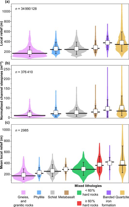
170                      D. Peifer et al.: Growing topography due to contrasting rock types in a tectonically dead landscape

Figure 2. The geomorphic context of the Quadrilátero Ferrífero, Brazil. (a) Map of local topographic relief (extracted using a 2 km diam-
eter window). (b) Simplified bedrock geology in the study area, comprising mostly steeply dipping (≥ 35◦ ) Archean and Paleoproterozoic
sequences. (c) Map of normalised channel steepness (ksn ) extracted using the segmentation method of Mudd et al. (2014), with θref of 0.45.
Note that we used an area threshold of 1.0 km2 to extract the drainage network, and we did not show sampling sites in (c) for illustration
purposes. (d) The location of the QF in Brazil, ∼ 350 km away (in a straight line) from the Atlantic Ocean.

The resulting 10 Be/9 Be ratios for each sample were cor-               shielding (DiBiase, 2018). We have also incorporated eight
rected for processed blank ratios (n = 2), ranging between              detrital 10 Be-derived concentration measurements previously
0.2 % and 3.2 % of the sample 10 Be/9 Be ratios, with uncer-            published for the QF (Salgado et al., 2008) in our dataset;
tainties propagated in quadrature (Balco et al., 2008).                 however, we recalculated denudation rates using the method
   Catchment-averaged denudation rates were derived from                described above to ensure consistency (Table S1 in the Sup-
10 Be concentrations using the CRONUS online calculator                 plement).
v3.0 (Balco et al., 2008). We used the CAIRN method (Mudd
et al., 2016) to quantify catchment-averaged pressure em-               3.2   Quantification of catchment-averaged geomorphic
ploying a pixel-by-pixel approach and recommended param-                      metrics
eters (Mudd et al., 2016). We report denudation rates using
the time-independent Lal/Stone scaling method (Lal, 1991;               We used a 12 m TanDEM-X (TerraSAR-X add-on for Digital
Stone, 2000) and assuming a standard bedrock density of                 Elevation Measurement) digital elevation model (DEM) to
2.7 g cm−3 (e.g. von Blanckenburg et al., 2004; Mandal et               extract the following topographic metrics: (i) local relief and
al., 2015). We have not applied corrections for topographic             (ii) normalised channel steepness. The WorldClim v2 dataset
                                                                        (Fick and Hijmans, 2017) was used to extract (iii) mean an-

Earth Surf. Dynam., 9, 167–181, 2021                                                        https://doi.org/10.5194/esurf-9-167-2021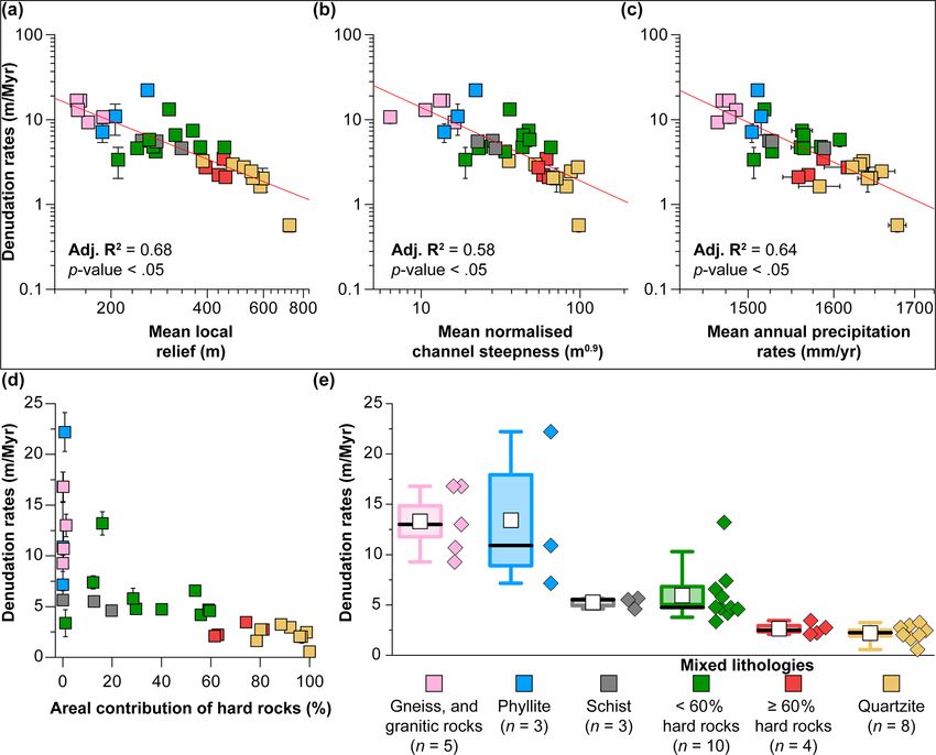
D. Peifer et al.: Growing topography due to contrasting rock types in a tectonically dead landscape                                   171

nual precipitation rates. These metrics have been demon-            Table 1. Variability in θ in the QF. Best-fit θ values were computed
strated to play an essential role in revealing the pattern and      for all catchments of a stream order higher than the third order based
style of landscape evolution in erosive settings (e.g. Ahnert,      on the disorder method (Hergarten et al., 2016) using code devel-
1970; Montgomery and Brandon, 2002; DiBiase et al., 2010;           oped by Mudd et al. (2018).
Portenga and Bierman, 2011; Harel et al., 2016). Catchments
were extracted from the DEM following standard hydrologi-                                                     Best-fit θ statistics
cal routing procedures using sample locations as pour points.               Stream order       Number of      Mean      Standard
Catchment-averaged values for each metric were determined                                         basins       θ        deviation
as the average of all local values within each catchment.
                                                                            Fourth-order              114      0.37        0.17
   Various authors have observed empirically that channel                   Fifth-order                24      0.45        0.12
slope (S) declines progressively as contributing drainage                   Sixth-order                 5      0.46        0.08
area (A) increases in the downstream direction of a channel                 Seventh-order               1      0.53         –
profile, in a relationship that can be described by a power law
(e.g. Flint, 1974):                                                         All catchments            144      0.44        0.13

S = ks A−θ ,                                                 (1)
                                                                    on θref . We quantified ksn as the derivative of χ and z (e.g.
where θ , termed the “channel concavity”, controls how              Mudd et al., 2014) instead of using regressions of slope area
rapidly channel slope decreases with increasing drainage            data (e.g. DiBiase et al., 2010; Kirby and Whipple, 2012) be-
area, and ks , referred to as the “channel steepness”, is a mea-    cause the integral method does not require estimating slope
sure of channel steepness normalised by upstream drainage           from the DEM, resulting in more precise ksn values (Perron
area, which has been demonstrated to correlate positively           and Royden, 2013). We estimated how θ varies over the study
with denudation rates in different geomorphic conditions            area based on the disorder method (Hergarten et al., 2016),
(e.g. DiBiase et al., 2010; Mandal et al., 2015; Harel et al.,      which was carried out using routines developed by Mudd et
2016). The parameters ks and θ covary, and this autocor-            al. (2018), to derive an optimal θ value for the entire land-
relation is corrected by defining a fixed reference concav-         scape. The drainage network was extracted using an area
ity (θref ), which is used to extract a normalised channel steep-   threshold of 0.5 km2 (e.g. Beeson et al., 2017; Campforts et
ness (ksn ) from the data (Kirby and Whipple, 2012).                al., 2020), which is lower than the minimum drainage area
   Equation (1) can be used to derive estimates of ks and θ         among the catchments where we collected fluvial sediments
(or ksn ) from regressions of log-transformed slope area data       (0.86 km2 ) and is a reasonable critical threshold for the study
(Kirby and Whipple, 2012). Alternatively, one can extract ksn       area (Fig. S2). We computed θ for all catchments of a stream
using an approach referred to as the integral method (Perron        order higher than the third order following Strahler (1957)
and Royden, 2013). For that, Eq. (1) is rearranged by replac-       (n = 144), covering the entire study area; these catchments
ing S with dz/dx and separating these variables, where z is         were extracted using code developed by Clubb et al. (2019).
elevation and x is distance along the channel, which is then        The mean θ for the QF (0.44; Table 1) is close to the fre-
integrated in the upstream direction from an arbitrarily base       quently used value of 0.45 (e.g. Mandal et al., 2015); thus,
level at xb , resulting in an equation for the elevation profile    we set 0.45 as the reference concavity from which we com-
(e.g. Mudd et al., 2018):                                           puted the normalised channel steepness employing the seg-
                          ! Zx           θ                        mentation method of Mudd et al. (2014).
                 ks                 A0                                  We quantified local relief as the elevation range within
z(x) = z (xb ) +                               dx,           (2)
                 Aθ0               A(x)                             a neighbourhood defined by a 2 km diameter circular win-
                              xb
                                                                    dow. The choice of the local relief window was based on
where A0 is a reference drainage area that is inserted to make      sensitivity analysis (DiBiase et al., 2010). We compared the
the area term dimensionless (Perron and Royden, 2013). One          goodness-of-fit in bivariate regressions between average val-
can then define a longitudinal coordinate chi (χ) with dimen-       ues of local relief (with window diameter varying from 0.5 to
sions of length using (Perron and Royden, 2013; Mudd et al.,        5.0 km) and normalised channel steepness for every catch-
2014):                                                              ment in the study area with a stream order higher than the
                                                                    second order. In this situation, the local relief obtained using
     Zx           θ                                               the 2 km diameter window exhibits the highest goodness-of-
             A0
χ=                      dx.                                  (3)    fit value (measured using the ordinary least squares method;
            A(x)                                                    Myers, 1990) with catchment-averaged normalised chan-
     xb
                                                                    nel steepness (Fig. S3), and it is therefore the one that
In the case of A0 = 1, the slope of a longitudinal profile in       has been used throughout. Finally, we extracted mean an-
a z versus χ plot is the channel steepness (ks ) or the nor-        nual precipitation rates from the 30 arcsec spatial resolution
malised channel steepness (ksn ) if the extraction is based         WorldClim v2 global monthly precipitation dataset for the

https://doi.org/10.5194/esurf-9-167-2021                                                    Earth Surf. Dynam., 9, 167–181, 2021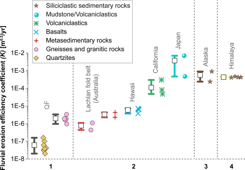
172                      D. Peifer et al.: Growing topography due to contrasting rock types in a tectonically dead landscape

years 1970 to 2000, which is based on raw weather station           runoff efficiency, channel width scaling, extreme hydrologic
data and covariates from satellite sensors that were interpo-       events, and frequency of debris flow (e.g. Snyder et al., 2000;
lated and combined, creating global climate surfaces (Fick          Whipple et al., 2000a; Kirby and Whipple, 2001; Duvall
and Hijmans, 2017).                                                 et al., 2004; Zondervan et al., 2020b). All of these factors
                                                                    are encapsulated in a dimensional coefficient of erosion ef-
3.3   Lithological strength and fluvial erosion efficiency in
                                                                    ficiency (K) in the commonly used stream power model
      the QF
                                                                    (Howard and Kerby, 1983):

The QF is characterised by the presence of vast ore de-             E = KAm S n ,                                               (4)
posits, particularly gold, iron and manganese (Dorr, 1969;
Lobato et al., 2001). The exploitation of these ore reserves        where E is the long-term fluvial erosion; A is the upstream
has led to focused research, and the QF is the most systemat-       contributing drainage area; S is the local channel gradient;
ically investigated geological domain in Brazil (Lobato et al.,     and m and n are positive exponents that depend on incision
2001). We extracted geological data from the “Projeto Ge-           process, channel hydraulics, and rainfall variability (Whipple
ologia do Quadrilátero Ferrífero” dataset mapped at a scale         and Tucker, 1999).
of 1 : 25 000 (Lobato et al., 2005).                                   Whereas most variables in the stream power model can be
   Rivers in the study area erode through a landscape marked        derived from DEM data, the fluvial erosion efficiency coef-
by variations in rock type, including granitic, argillaceous,       ficient (K) cannot be measured directly, and thus the com-
quartzose and carbonate rocks, as well as iron formations.          puting of K demands constraints on timing and/or rates of
These rock units are metamorphosed and steeply dipping as           river evolution (Zondervan et al., 2020b). We have a limited
a result of QF’s polyphase deformation history (Dorr, 1969;         understanding of how K varies in different geomorphic con-
Chemale et al., 1994; Alkmim and Marshak, 1998). There is           ditions and what controls its variability due to the few stud-
a clear consensus from geological research that the exposed         ies that derived absolute constraints on K and confounding
lithologies have differential resistance to weathering and ero-     between the multiple controls encoded in K (Snyder et al.,
sion, whereby quartzites, banded iron formations, and iron          2000; Whipple et al., 2000a; Duvall et al., 2004; Harel et al.,
duricrusts comprise the most resistant lithologies; schists,        2016; Zondervan et al., 2020b). More sophisticated versions
phyllites, dolomitic units, and metavolcanics rocks are less        of the stream power model may explicitly account for differ-
resistant lithologies; and gneisses and granitic rocks are the      ent controls in K (e.g. DiBiase and Whipple, 2011; Camp-
least resistant rocks exposed in the QF (e.g. Dorr, 1969; Sal-      forts et al., 2020; Zondervan et al., 2020b), yet such an ap-
gado et al., 2008; Monteiro et al., 2018; Vasconcelos and           proach requires specific data of an adequate resolution, such
Carmo, 2018). Following the approach taken by previous              as river hydraulic geometry, rock strength measurements, and
studies (e.g. Lague et al., 2000; Korup, 2008; Jansen et al.,       hydrological data to resolve spatial and temporal runoff vari-
2010; Hurst et al., 2013), we assumed that such classification      ability, which are not readily available.
of rock strength as a function of rock type is valid, although         We computed catchment-averaged values of K for the
we do not have rock strength measurements to support it.            QF using an approach similar to Gallen (2018) based on ksn
Given the humid subtropical condition of the QF, we expect          and average erosion rates. Such an approach requires that
differential resistance to reflect variations in the susceptibil-   spatial variability in long-term rock uplift over the study area
ity to chemical weathering of the different rock units (Mey-        is low, which is a reasonable assumption for the QF. Rear-
beck, 1987; White and Blum, 1995). For instance, gneisses           ranging Eq. (4) to solve for channel slope can cast the stream
and granitic rocks with an abundant presence of feldspars are       power model in the same form as Eq. (1):
readily weathered, whereas physically robust and chemically                     1/n
                                                                             E
inert quartzites weather much more slowly via the intergran-        S=                  A−m/n ,                                 (5)
ular solution of quartz (Dorr, 1969). In general in the study                K
area, quartzites and banded iron formations form pronounced         where
ridges and steep landforms with relatively unweathered out-
                                                                           1/n
crops compared to areas in gneisses and granitic rocks asso-                E
ciated with broad lowlands that are deeply weathered, with          ksn =        ,                                              (6)
                                                                            K
regolith extending to depths of 50 m or more (e.g. Dorr, 1969;
                                                                    θref = m/n,                                                 (7)
Salgado et al., 2008).
   Theory and field observations demonstrate that rock              and thus
strength influences long-term fluvial incision rates in ero-
sive settings (e.g. Gilbert, 1877; Howard and Kerby, 1983;                n
                                                                    E = Kksn .                                                  (8)
Stock and Montgomery, 1999; Whipple and Tucker, 1999;
Jansen et al., 2010; Bursztyn et al., 2015) in concert with a       We extracted ksn using 0.45 as the reference concavity, which
number of other controls, including climate conditions and          assuming m = 0.45 and n = 1 yields K values with units

Earth Surf. Dynam., 9, 167–181, 2021                                                       https://doi.org/10.5194/esurf-9-167-2021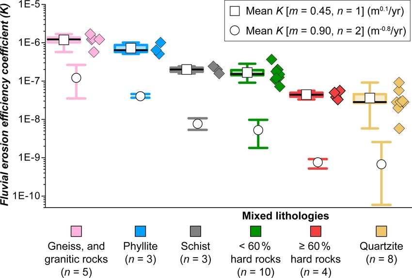
D. Peifer et al.: Growing topography due to contrasting rock types in a tectonically dead landscape                              173

of m0.1 yr−1 . We assumed that catchment-wide denudation
rates derived from detrital 10 Be concentrations are represen-
tative of long-term fluvial incision in the QF, considering that
there are no records of the occurrence of deep-seated land-
slides (Dorr, 1969) and that sampled catchments are of a rea-
sonable size. We calculated K assuming n = 1 and n = 2,
which have been previously demonstrated as feasible values
of n (Lague, 2014). In the study area, the range of precip-
itation is relatively low (from 1356 to 1729 mm yr−1 ), with
areas of higher elevations principally underlain by resistant
rocks receiving more precipitation than valley bottoms in
more erodible rock units (Fig. S4), indicating opposing ef-
fects in K between inferred rock strength and precipitation
rates. We explored how rock type and precipitation rates are
linked to catchment-averaged values of K.

4     Results

4.1    Catchment-averaged denudation rates in the QF

Catchment-averaged denudation rates in the study area range
from 0.6 ± 0.1 to 22.2 ± 1.9 m Myr−1 , with a regional mean
denudation rate of 6.4 m Myr−1 (Fig. 3; Table S1). Denuda-
tion rates in the QF are thus comparable to or lower than
previous estimates of denudation rates in other tectonically
inactive, post-orogenic settings (e.g. Harel et al., 2016), in-
cluding the Cape Mountains (e.g. Scharf et al., 2013), the Ap-
palachian Mountains (e.g. Matmon et al., 2003), the Ozark          Figure 3. Catchment-averaged denudation rates in the study area
dome (e.g. Beeson et al., 2017), the Sri Lankan uplands (e.g.      draped over a hillshade image. Note that we identify the 25 sam-
von Blanckenburg et al., 2004) and the Western Ghats (e.g.         pling sites of this study with “P” followed by a number, whereas we
Mandal et al., 2015). However, denudation rates are not uni-       label the 8 sampling sites incorporated from Salgado et al. (2008)
formly low in the study area, varying by more than an order        with “S” followed by a number. See Table S1 for 10 Be analytical
of magnitude (Fig. 3), from the slowly denuding catchments         results and derived denudation rate data.
in the eastern part of the QF, where all catchments exhibit
denudation rates lower than 3.5 m Myr−1 , to the western part
of the QF where catchments are eroding at higher rates up to       mean annual precipitation (Fig. 4c), contrary to the expec-
22.2 ± 1.9 m Myr−1 (Fig. 3).                                       tation that wetter climates drive more rapid denudation (e.g.
                                                                   Moon et al., 2011; Harel et al., 2016), and finally we find
4.2    Links between topographic metrics, precipitation
                                                                   a weak correlation between catchment-averaged denudation
       rates, rock type, and denudation rates
                                                                   rates and catchment area (Fig. S5). However, we observe that
                                                                   catchment-averaged denudation rates may increase together
We find that catchment-averaged denudation rates are nega-         with mean values of topographic metrics and precipitation
tively correlated with mean values of local relief (Fig. 4a),      rates for individual rock types, although with such small sam-
contrary to the established understanding of links between         ple sizes no such relationships are statistically significant at
denudation and topographic relief and the bulk of support-         the α = 0.05 level except for catchments in phyllites (Figs. 4
ing empirical studies (e.g. Ahnert, 1970; Montgomery and           and S6).
Brandon, 2002; DiBiase et al., 2010; Harel et al., 2016). Sim-        Denudation rates can instead be linked to inferred rock
ilarly, catchment-averaged denudation rates are negatively         strength (Fig. 4e). Catchments underlain by quartzites are as-
correlated with mean values of normalised channel steep-           sociated with the slowest denudation rates (from 0.6 ± 0.1 to
ness (Fig. 4b), a parameter often used to infer denudation         3.3 ± 0.3 m Myr−1 , with a mean of 2.2 m Myr−1 ). Catch-
rates based on the empirical positive correlation between de-      ments in mixed lithologies where ≥ 60 % of catchment area
nudation and normalised channel steepness in tectonically          consists of resistant lithologies denude at slightly higher
active landscapes (e.g. DiBiase et al., 2010; Kirby and Whip-      rates up to 3.5 ± 0.3 m Myr−1 (with a mean of 2.6 m Myr−1 ).
ple, 2012; Harel et al., 2016). We also find a negative rela-      In contrast, catchments in less resistant schists or mixed
tionship between catchment-averaged denudation rates and           lithologies with < 60 % of resistant lithologies denude more

https://doi.org/10.5194/esurf-9-167-2021                                                 Earth Surf. Dynam., 9, 167–181, 2021
174 D. Peifer et al.: Growing topography due to contrasting rock types in a tectonically dead landscape
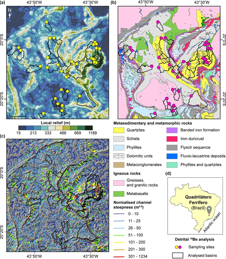
Figure 4. Links between denudation rates, geomorphic parameters, and rock type in the study area. Variations in catchment-averaged
denudation rates with (a) mean local relief, (b) mean normalised channel steepness, (c) mean annual precipitation rates, and (d) percentage
areal contribution of resistant rocks. Error bars on the y axis show measurement uncertainties in the nuclide concentration, as well as
uncertainties related to the scaling method, and error bars on the x axis indicate the standard error of the mean. (e) Variations in catchment-
averaged denudation rates per rock type, with the box on the left and raw data (diamonds) on the right. Box range represents the standard
error of the mean, whiskers show the interval between the 10th and 90th percentiles of the data, white squares show mean values, and
thick black lines exhibit median values. Mixed lithology refers to catchments where a single lithology does not account for ≥ 75 % of the
catchment area.
rapidly. Finally, the low-relief catchments underlain by the sistant rocks. However, the low end of the distribution of to-
least resistant (under humid subtropical climate conditions) pographic metrics shows comparably low values for every
gneisses and granitic rocks, as well as catchments domi- rock type, which indicates that subdued local relief and chan-
nated by phyllites, denude at higher rates of up to 22.2 ± nel steepness occur on all lithologies. We also find positive
1.9 m Myr−1 . Similarly, we observe that a higher percent- relationships between catchment-averaged topographic relief
age contribution of resistant rocks in the catchment area (i.e. and inferred rock strength (Fig. 5c). In particular, we observe
areas in quartzites and banded iron formations) determines that catchments in mixed lithologies where ≥ 60 % of catch-
lower rates of denudation (Fig. 4d). ment area consists of resistant lithologies exhibit substan-
The regional distribution of topographic metrics indicates tially higher local relief than catchments in mixed lithologies
a positive correlation between topography and inferred rock with less than 60 % of resistant lithologies.
strength (Fig. 5). In this situation, the high end of the distri-
bution of topographic metrics, as well as mean and median
4.3 Fluvial erosion efficiency and its relationships with
values, exhibits similar trends of high values for areas un-
rock type and precipitation rates
derlain by quartzites and banded iron formations; intermedi-
ate values for less resistant rock types such as metabasalts, Assuming the slope exponent n = 1, we find that the flu-
schists, and phyllites; and low values for areas underlain by vial erosion efficiency coefficient (K) differs by 3 orders
the least resistant basement rocks, which are also marked by of magnitude in the study area, varying from 5.8 × 10⁻⁹ to
lower variability in topography than areas dominated by re- 1.7 × 10⁻⁶ m0.1 yr−1 , with a mean of 3.3 × 10⁻⁷ m0.1 yr−1
Earth Surf. Dynam., 9, 167–181, 2021 https://doi.org/10.5194/esurf-9-167-2021D. Peifer et al.: Growing topography due to contrasting rock types in a tectonically dead landscape 175
Figure 6. Lithology controls the fluvial erosion efficiency coeffi-
cient (K) in the study area. Boxplot elements are as follows: box
range represents the standard error of the mean, whisker range
shows the interval between the 10th and 90th percentiles of the data,
and the thick black line shows the median values. Note that we cal-
culated K assuming (i) m = 0.45 and n = 1 (derived values of K
have units of m0.1 yr−1 ) and (ii) m = 0.9 and n = 2 (derived values
of K have units of m−0.8 yr−1 ). For the case of n = 1, we show
the boxplot on the left and raw data (diamonds) on the right. See
Table S1 for data on each of the catchments analysed, including
lithology and mean annual precipitation rates.
shows that K is statistically different in catchments under-
lain by different rock types at the α = 0.01 level. When the
slope exponent n is equal to 2, we find absolute values of K
to be more than 1 order of magnitude lower for every catch-
ment (assuming m = 0.9 and n = 2, derived values of K
have units of m−0.8 yr−1 ). Nevertheless, the same relation-
Figure 5. Lithology controls topographic forms in the study area. ship with rock type as observed for the case of n equal to 1
Violin plots show the probability density (smoothed by a ker- emerges, with low values of K associated with quartzites and
nel density estimator), per rock type, of (a) local relief, (b) nor- orders of magnitude higher K values in areas in gneisses and
malised channel steepness, and (c) catchment-averaged local re- granitic rocks (Fig. 6). Finally, although the spatial variability
lief. Panels (a) and (b) represent the distribution of local relief in rainfall is limited in the study area, we observe that catch-
and normalised channel steepness for the entire study area, whereas ments that receive more precipitation (in higher elevations
panel (c) shows mean values of local relief for all catchments with a underlain by resistant rocks) are associated with substantially
stream order equal or higher than the second order (Strahler, 1957)
lower K values than areas that receive less precipitation (in
underlain by the rock types represented in (a)–(c). Whiskers show
the interval between the 10th and 90th percentiles of the data, white
more erodible rock units) (Fig. S7).
squares represent mean values, and thick black lines exhibit median
values. 5 Discussion
5.1 Equilibrium as a natural attractor state in a decaying
−7 mountain belt
and a standard deviation of 4.5 × 10 m0.1 yr−1
(Fig. 6;
Table S1). Our results indicate that K decreases substan- Our results show that bedrock strength controls the variabil-
tially with increasing inferred rock strength, varying from ity in topographic relief and channel steepness in the QF. This
low K values in areas underlain by quartzites (with a mean K conclusion is consistent with the classic geomorphic expec-
of 3.6 × 10⁻⁸ m0.1 yr−1 ) to considerably higher K values tation that, all else being equal, terrains underlain by resis-
in areas in gneisses and granitic rocks (with a mean K of tant rocks will develop higher topographic relief and steeper
1.2 × 10⁻⁶ m0.1 yr−1 ) (Fig. 6). We observe some degree of channel gradients (e.g. Gilbert, 1877; Hack, 1960; Jansen et
overlap between K values for catchments consisting of dif- al., 2010; Bursztyn et al., 2015). Such correlation between
ferent rock types (Fig. 6). However, a Kruskal–Wallis test topographic forms and rock strength is the same as that ex-
https://doi.org/10.5194/esurf-9-167-2021 Earth Surf. Dynam., 9, 167–181, 2021176 D. Peifer et al.: Growing topography due to contrasting rock types in a tectonically dead landscape
pected in an equilibrium adjustment scenario for a tecton-
ically stable erosive landscape evolving over timescales of
millions of years (Hack, 1960; Montgomery, 2001). In the
case of a spatially variable lithological configuration, the-
ory predicts that more erodible rock units are progressively
eroded, whereas resistant rocks stand proud in relief, up to
a point where differential topographic steepness everywhere
balances spatial variations in rock strength, and denudation
rates are then spatially invariant (Hack, 1960). Our detrital
cosmogenically-derived results, however, demonstrate that
rates of denudation are kept spatially variable by the ex-
posure at the surface of different rock types in a tectoni-
cally inactive landscape evolving for hundreds of millions
of years. The landscape has not achieved any equilibrium or
a steady state. We interpret our findings as an indication that
equilibrium is likely not a natural attractor state in decaying Figure 7. Comparison of our results for the fluvial erosion effi-
ciency coefficient (K) with previously published estimates of K.
mountain belts or is (at best) an attractor state that cannot be
Note that we display whiskers (representing the interval between
reached as long as lithological spatial heterogeneity (such as the 10th and 90th percentiles of the data) and mean values (white
the one observed in the study area) is maintained, a conclu- squares) on the left and raw data (diamonds) on the right. Estimates
sion that is consistent with the modelling results of Forte et of K were derived assuming the slope exponent n = 1. Numbers on
al. (2016). the x axis represent different data sources: (1) this study; (2) Stock
and Montgomery (1999); (3) Whipple et al. (2000b); (4) Kirby and
Whipple (2001). Lithology was compiled as described by the re-
5.2 Lateral variations in rock type as a dominant control
spective authors of the above studies.
on denudation rates and topographic forms in a
post-orogenic landscape
Our results suggest that the fluvial erosion efficiency coeffi- accounts for the magnitude of variations in the fluvial ero-
cient (K) varies as a function of rock type in the study area, sion efficiency coefficient (K) estimated for the study area.
with low K values in resistant units and orders of magni- Our findings agree with studies that demonstrate that the link
tude higher K values in more erodible rocks. In contrast, we between denudation rates and channel steepness is obscure in
find that spatial gradients in precipitation rates do not con- settings where lateral variations in rock strength are impor-
trol changes in K in the study area, considering that wet- tant (e.g. Cyr et al., 2014; Campforts et al., 2020) and that
ter climate conditions are generally associated with higher a modified version of the stream power model that includes
values of K (e.g. Ferrier et al., 2013). However, the fluvial variations in rock strength should be adopted for better pre-
erosion efficiency coefficient (K) as calculated here incor- dicting spatial patterns of channel incision (Campforts et al.,
porates other effects besides rock strength and precipitation 2020). Our results imply that modelling studies attempting
rates, such as channel hydraulic geometry and sediment load to reconstruct uplift histories from river profile morphology
(e.g. Snyder et al., 2000; Duvall et al., 2004; Zondervan et assuming uniform fluvial erosion efficiency over large areas
al., 2020b). Whereas in the Appalachians effects on fluvial (e.g. Roberts and White, 2010) are likely to be flawed (at
erosional efficiency such as channel width and sediment load least in post-orogenic settings).
have been shown to vary as a function of rock type (e.g. To compare our constraints on the fluvial erosion effi-
Spotila et al., 2015), we do not have data on such variables ciency coefficient with published estimates of K, we also
for the QF, which is a limitation to our reasonable interpre- calculate K in units of m0.2 yr−1 , as reported in several
tation that rock type controls K in the study area. We note, studies (e.g. Stock and Montgomery, 1999; Whipple et al.,
however, that rock strength varies within each rock type in 2000b; Kirby and Whipple, 2001). We find that the result-
the study area, and, for instance, thin-bedded quartzites with ing estimates of K in the QF (regional mean K value of
large quantities of muscovite and sericite weather and erode 7.1×10⁻⁷ m0.2 yr−1 , assuming the slope exponent n = 1) are
much more easily than average, while some granitic areas comparable to or lower than the low end of the K values re-
stand bold in relief where these rocks are coarser-grained and ported by Stock and Montgomery (1999) for a post-orogenic
more massive (Dorr, 1969). landscape underlain by granites and metasedimentary rocks
The negative relationships we find between 10 Be- in humid subtropical Australia (Fig. 7). Similarly, our esti-
derived catchment-averaged denudation rates and catchment- mates of K (in Fig. 6) are comparable to or lower than the
averaged values of topographic relief, channel steepness and low end of the K values estimated in crystalline and meta-
precipitation rates are counter-intuitive. However, such rela- morphic rocks in the upper Tennessee River (mean K val-
tionships are consistent with the stream power model if one ues of ∼ 5 × 10⁻⁷ m0.1 yr−1 ; Gallen, 2018), as well as in dif-
Earth Surf. Dynam., 9, 167–181, 2021 https://doi.org/10.5194/esurf-9-167-2021D. Peifer et al.: Growing topography due to contrasting rock types in a tectonically dead landscape 177
ferent physiographic provinces in the Appalachians such as Extrapolation of the denudation pattern in the QF over
the Blue Ridge (reported K values: 7.8–3.0×10⁻⁷ m0.1 yr−1 ; time, which is speculative for timescales more extended than
Gallen et al., 2013) and the Valley and Ridge (reported K val- the averaging of our cosmogenic data (Table S1), suggests
ues: 2.1–1.5 × 10⁻⁶ m0.1 yr−1 ; Miller et al., 2013). In con- that exposure at the surface of rocks with significant con-
trast, our results are orders of magnitude lower than estimates trasts in erodibility naturally favours the survival of relief
of K in tectonically active areas in Hawaii (tropical rainfor- in the absence of ongoing tectonics. Nevertheless, we have
est climate), California (Mediterranean climate), and Japan compelling geomorphic evidence that at least some decay-
(humid continental climate; Stock and Montgomery, 1999), ing mountain belts underwent spatial and temporal changes
as well as the Siwalik Hills in the Himalayas (monsoon high- in denudation rates as a response to different types of forc-
land climate; Kirby and Whipple, 2001) and the Ukak River ing (e.g. tectonic, lithologic, climatic, mantle-driven, and far-
in Alaska (cool continental climate; Whipple et al., 2000b). field-driven) long after cessation of crustal thickening (e.g.
It is difficult to isolate the influence of rock strength from Pazzaglia and Brandon, 1996; Quigley et al., 2007; Gallen et
climate conditions in this comparison. Nonetheless, Fig. 7 al., 2013; Tucker and van der Beek, 2013; Liu, 2014; Gallen,
suggests a stark contrast over orders of magnitude in the flu- 2018). In this situation, large spatial contrasts in the fluvial
vial erosion efficiency coefficient between tectonically ac- erosion efficiency coefficient (K), such as observed in our
tive and inactive settings, which may result from the dispar- study area, determine significant differences in erosional re-
ity between the high rates of denudation in orogenic belts, sponse times across the landscape (i.e. the timescale of chan-
with exposure of mineral surfaces that are readily weath- nel profile response to perturbations in boundary conditions),
ered, and the long timescales of evolution in ancient moun- with response times (Td ) decreasing as K increases (Td scales
tain belts, where the hard metamorphic roots of these land- to 1/K n , where n is the slope exponent in the stream power
scapes are progressively exhumed as these landscapes age model; Baldwin et al., 2013). Spatial gradients in K thus con-
(Summerfield and Hulton, 1994; Bishop, 2007; Braun et al., trol how post-orogenic landscapes respond to a given force.
2014; Bursztyn et al., 2015). In contrast, the global dataset Indeed, lithological controls on post-orogenic landscape dy-
of stream power model parameters reported by Harel et al. namics have long been identified (e.g. Hack, 1960, 1975;
(2016) exhibits lower K values in tectonically active areas Twidale, 1976; Mills, 2003; Bishop and Goldrick, 2010;
compared to higher K values in inactive settings. These au- Spotila et al., 2015; Gallen, 2018; Bernard et al., 2019; Vas-
thors concluded that such results were counter-intuitive and concelos et al., 2019; Zondervan et al., 2020a). Nonetheless,
highlighted the fact that K is not well calibrated (Harel et al., lithological contrasts have not been addressed adequately by
2016); more work needs to be dedicated to the determination numerical modelling of post-orogenic landscape evolution
of K and what controls its variations. and, in particular, topographic decay (e.g. Baldwin et al.,
2003; Egholm et al., 2013).
5.3 Landscape development in a decaying mountain
belt marked by lateral contrasts in rock strength
6 Conclusion
Our findings indicate that high-relief uplands underlain by
resistant bedrock are denuding more slowly than lower-relief We present 10 Be concentrations in river sand from catch-
surrounding areas associated with more erodible litholo- ments spanning the range of topographic metrics and bedrock
gies, with the corollary that topographic relief must still be erodibility in a humid subtropical, tectonically inactive land-
growing instead of decaying in this tectonically quiescent scape in Brazil. The results of this study suggest that the
landscape. Furthermore, the expected isostatic compensation post-orogenic history of the study area is not a progressive
to denudational unloading (e.g. Bishop and Brown, 1992), reduction in relief and denudation rates. Instead, the expo-
which is a process that occurs at a much longer wavelength sure at the surface of rocks with strong lateral contrasts in
than the local changes in lithology and denudation rates erodibility amplifies spatial differences in topographic forms
(Gilchrist and Summerfield, 1990; Watts et al., 2000), im- and denudation rates over time, sustaining or indeed increas-
plies that uplands and surrounding areas are equally isostat- ing relief in a tectonically dead landscape. Spatial variations
ically uplifted in response to the regional denudation, likely in topographic relief and channel steepness are explained by
resulting in a net reduction of mean elevation over time but a changes in rock type in the study area, and yet denudation
slight increase in the heights of mountain peaks, as has been rates are not spatially uniform. Contrasts in rock type con-
proposed by Molnar and England (1990). The timescale over tinue to drive differences in denudation rates in a decay-
which relief might continue to grow simply as a result of spa- ing mountain belt evolving over a timescale of millions of
tial variations in bedrock lithology is unresolved. However, years, indicating that the landscape has not achieved equilib-
our results suggest that relief is likely to persist long into the rium. This study demonstrates that lateral variations in rock
future in a landscape that would otherwise be suited to rapid strength play an essential role in the dynamics of an ancient
denudation (high-relief and relatively high precipitation rates mountain belt, and likely in other post-orogenic settings char-
and warm climate). acterised by spatial heterogeneity in lithology. Such litholog-
https://doi.org/10.5194/esurf-9-167-2021 Earth Surf. Dynam., 9, 167–181, 2021178 D. Peifer et al.: Growing topography due to contrasting rock types in a tectonically dead landscape
ical heterogeneity controls the tempo and style of landscape Alvares, C. A., Stape, J. L., Sentelhas, P. C., de Moraes Gonçalves,
response to changes in boundary conditions while also af- J. L., and Sparovek, G.: Köppen’s climate classification map for
fecting the pattern of landscape denudation. Brazil, Meteorol. Z., 22, 711–728, https://doi.org/10.1127/0941-
2948/2013/0507, 2013.
Balco, G., Stone, J. O., Lifton, N. A., and Dunai, T. J.:
Data availability. The data supporting the findings of this study A complete and easily accessible means of calculating
are available in the Supplement, including 10 Be analytical re- surface exposure ages or erosion rates from 10 Be and
26 Al measurements, Quat. Geochronol., 3, 174–195,
sults and derived denudation rate data, catchment-averaged geo-
morphic parameters, and detailed information on catchment lithol- https://doi.org/10.1016/j.quageo.2007.12.001, 2008.
ogy. Extraction of topographic metrics and catchment-averaged Baldwin, J. A., Whipple, K. X., and Tucker, G. E.: Implications of
pressure were carried out using LSDTopoTools version 2.03 the shear stress river incision model for the timescale of postoro-
(https://doi.org/10.5281/zenodo.3769703, Mudd et al., 2020). genic decay of topography, J. Geophys. Res.-Solid, 108, 1–17,
https://doi.org/10.1029/2001JB000550, 2003.
Barreto, H. N., Varajão, C. A., Braucher, R., Bourlès, D. L., Sal-
gado, A. A., and Varajão, A. F.: Denudation rates of the Southern
Supplement. The supplement related to this article is available
Espinhaço Range, Minas Gerais, Brazil, determined by in situ-
online at: https://doi.org/10.5194/esurf-9-167-2021-supplement.
produced cosmogenic beryllium-10, Geomorphology, 191, 1–13,
https://doi.org/10.1016/j.geomorph.2013.01.021, 2013.
Beeson, H. W., McCoy, S. W., and Keen-Zebert, A.: Ge-
Author contributions. DP designed the study with contributions ometric disequilibrium of river basins produces long-lived
from all co-authors. DP and DF performed the cosmogenic isotope transient landscapes, Earth Planet. Sc. Lett., 475, 34–43,
analysis. DP quantified the geomorphic parameters. DP, CP, MDH, https://doi.org/10.1016/j.epsl.2017.07.010, 2017.
PB and DF wrote the manuscript. DP produced the figures. Bernard, T., Sinclair, H. D., Gailleton, B., Mudd, S. M., and Ford,
M.: Lithological control on the post-orogenic topography and
erosion history of the Pyrenees, Earth Planet. Sc. Lett., 518, 53–
Competing interests. The authors declare that they have no con- 66, https://doi.org/10.1016/j.epsl.2019.04.034, 2019.
flict of interest. Bierman, P. R. and Caffee, M.: Slow rates of rock surface
erosion and sediment production across the Namib Desert
and escarpment, southern Africa, Am. J. Sci., 301, 326–358,
Acknowledgements. We thank the German Aerospace Cen- https://doi.org/10.2475/ajs.301.4-5.326, 2001.
ter (DLR), the Natural Environment Research Council (NERC), and Bishop, P.: Long-term landscape evolution: linking tectonics
the Coordination for the Improvement of Higher Education Person- and surface processes, Earth Surf. Proc. Land., 32, 329–365,
nel (CAPES) for research support. We thank Hugh D. Sinclair for https://doi.org/10.1002/esp.1493, 2007.
providing feedback on an early version of the manuscript. Bishop, P. and Brown, R.: Denudational isostatic re-
bound of intraplate highlands: the Lachlan River val-
ley, Australia, Earth Surf. Proc. Land., 17, 345–360,
Financial support. The DLR granted us access to TanDEM- https://doi.org/10.1002/esp.3290170405, 1992.
X data as part of the project DEM_GEOL1345. NERC sup- Bishop, P. and Goldrick, G.: Lithology and the evolution of bedrock
ported the cosmogenic isotope analysis under CIAF award rivers in post-orogenic settings: constraints from the high-
no. 9177.0417. Daniel Peifer had support from CAPES under a elevation passive continental margin of SE Australia, Geol. Soc.
Science without Borders fellowship (grant no. BEX 12000/13-2) Spec. Publ., 346, 267–287, https://doi.org/10.1144/SP346.14,
and subsequently a CAPES-PrInt Postdoctoral fellowship (grant 2010.
no. 88887.367976/2019-00). Blackburn, T., Ferrier, K. L., and Perron, J. T.: Coupled feed-
backs between mountain erosion rate, elevation, crustal tem-
perature, and density, Earth Planet. Sc. Lett., 498, 377–386,
https://doi.org/10.1016/j.epsl.2018.07.003, 2018.
Review statement. This paper was edited by Greg Hancock and
Braun, J., Simon-Labric, T., Murray, K. E., and Reiners, P. W.: To-
reviewed by one anonymous referee.
pographic relief driven by variations in surface rock density, Nat.
Geosci., 7, 534–540, https://doi.org/10.1038/NGEO2171, 2014.
Bursztyn, N., Pederson, J. L., Tressler, C., Mackley, R. D.,
References and Mitchell, K. J.: Rock strength along a fluvial tran-
sect of the Colorado Plateau–quantifying a fundamental con-
Ahnert, F.: Functional relationships between denudation, relief, and trol on geomorphology, Earth Planet. Sc. Lett., 429, 90–100,
uplift in large, mid-latitude drainage basins, Am. J. Sci., 268, https://doi.org/10.1016/j.epsl.2015.07.042, 2015.
243–263, https://doi.org/10.2475/ajs.268.3.243, 1970. Campforts, B., Vanacker, V., Herman, F., Vanmaercke, M.,
Alkmim, F. F. and Marshak, S.: Transamazonian orogeny in Schwanghart, W., Tenorio, G. E., Willems, P., and Govers, G.:
the Southern Sao Francisco craton region, Minas Gerais, Parameterization of river incision models requires accounting for
Brazil: evidence for Paleoproterozoic collision and collapse environmental heterogeneity: insights from the tropical Andes,
in the Quadrilátero Ferrífero, Precambrian Res., 90, 29–58,
https://doi.org/10.1016/S0301-9268(98)00032-1, 1998.
Earth Surf. Dynam., 9, 167–181, 2021 https://doi.org/10.5194/esurf-9-167-2021You can also read