Performance Evaluation of GIS-Based Novel Ensemble Approaches for Land Subsidence Susceptibility Mapping - Frontiers
←
→
Page content transcription
If your browser does not render page correctly, please read the page content below
ORIGINAL RESEARCH
                                                                                                                                             published: 13 May 2021
                                                                                                                                     doi: 10.3389/feart.2021.663678

                                             Performance Evaluation of
                                             GIS-Based Novel Ensemble
                                             Approaches for Land Subsidence
                                             Susceptibility Mapping
                                             Alireza Arabameri 1 , Saro Lee 2,3* , Fatemeh Rezaie 2,3 , Subodh Chandra Pal 4 ,
                                             Omid Asadi Nalivan 5 , Asish Saha 4 , Indrajit Chowdhuri 4 and Hossein Moayedi 6,7
                                             1
                                               Department of Geomorphology, Tarbiat Modares University, Tehran, Iran, 2 Geoscience Platform Research Division, Korea
                                             Institute of Geoscience and Mineral Resources (KIGAM), Daejeon, South Korea, 3 Department of Geophysical Exploration,
                                             Korea University of Science and Technology, Daejeon, South Korea, 4 Department of Geography, The University of Burdwan,
                            Edited by:       Bardhaman, India, 5 Department of Watershed Management, Gorgan University of Agricultural Sciences and Natural
                       Hong Haoyuan,         Resources (GUASNR), Gorgan, Iran, 6 Informetrics Research Group, Ton Duc Thang University, Ho Chi Minh City, Vietnam,
          University of Vienna, Austria      7
                                               Faculty of Civil Engineering, Ton Duc Thang University, Ho Chi Minh City, Vietnam
                       Reviewed by:
                        Artemi Cerdà,
         University of Valencia, Spain
                                             The optimal prediction of land subsidence (LS) is very much difficult because of
                        Amiya Gayen,         limitations in proper monitoring techniques, field-base surveys and knowledge related
          University of Calcutta, India
                                             to functioning and behavior of LS. Thus, due to the lack of LS susceptibility maps
                           Lanh Ho Si,
   University of Transport Technology,       it is almost impossible to identify LS prone areas and as a result it influences severe
                              Vietnam        economic and human losses. Hence, preparation of LS susceptibility mapping (LSSM)
                  *Correspondence:           can help to prevent natural and human catastrophes and reduce the economic damages
                            Saro Lee
                  leesaro@kigam.re.kr
                                             significantly. Machine learning (ML) techniques are becoming increasingly proficient in
                                             modeling purpose of such kinds of occurrences and they are increasing used for LSSM.
                   Specialty section:        This study compares the performances of single and hybrid ML models to preparation
         This article was submitted to
            Environmental Informatics
                                             of LSSM for future prediction of performance analysis. In this study, the spatial prediction
                and Remote Sensing,          of LS was assessed using four ML models of maximum entropy (MaxEnt), general
               a section of the journal
                                             linear model (GLM), artificial neural network (ANN) and support vector machine (SVM).
            Frontiers in Earth Science
                                             Alongside, the possible numbers of novel ensemble models were integrated through
        Received: 03 February 2021
           Accepted: 08 April 2021           the aforementioned four ML models for optimal analysis of LSSM. An inventory LS map
           Published: 13 May 2021            was prepared based on the previous occurrences of LS points and the dataset were
                             Citation:       divvied into 70:30 ratios for training and validating of the modeling process. To identify
        Arabameri A, Lee S, Rezaie F,
    Chandra Pal S, Asadi Nalivan O,
                                             the robust and best LSSMs, receiver operating characteristic-area under curve (ROC-
 Saha A, Chowdhuri I and Moayedi H           AUC) curve was employed. The ROC-AUC result indicated that ANN model gives the
      (2021) Performance Evaluation
                                             highest ROC-AUC (0.924) in training accuracy. The highest AUC (0.823) of the LSSMs
       of GIS-Based Novel Ensemble
   Approaches for Land Subsidence            was determined based on validation datasets identified by SVM followed by ANN-SVM
              Susceptibility Mapping.        (0.812).
          Front. Earth Sci. 9:663678.
    doi: 10.3389/feart.2021.663678           Keywords: Geohazards, land subsidence, remote sensing, Kashan plain, machine learning

Frontiers in Earth Science | www.frontiersin.org                                  1                                             May 2021 | Volume 9 | Article 663678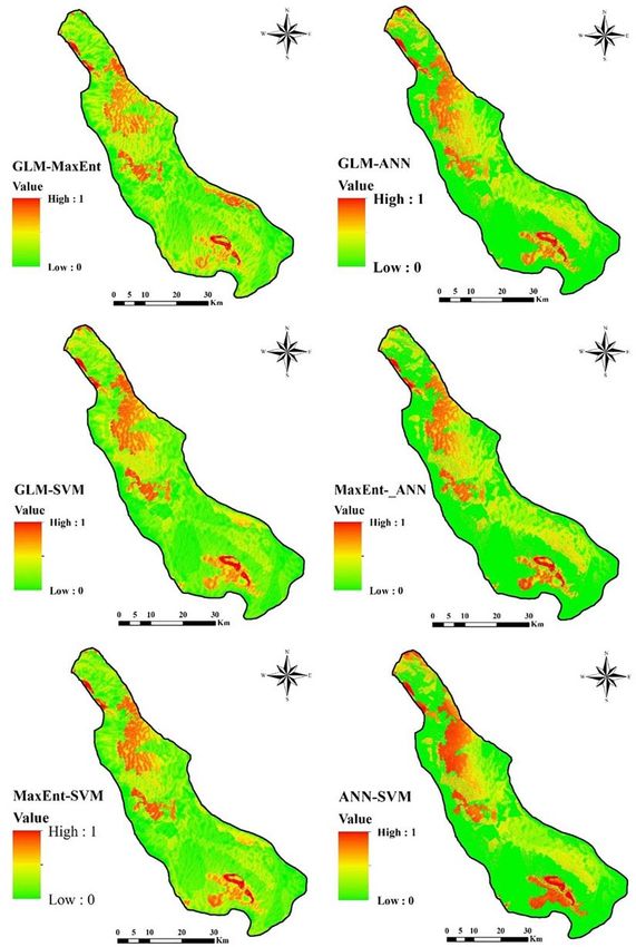
Arabameri et al.                                                                                          Performance Evaluation of GIS-Based Novel

INTRODUCTION                                                               The Phenomenon of climate change significantly increases the
                                                                           atmospheric temperature, as a result drought condition have
Land subsidence (LS) is a natural geo-hazard phenomenon that               been occurred and a large number of people greatly depends
occurs around the globe and causes extensive deformation of the            on groundwater, and gradually destruction of aquifers causes
earth’s surface. More specifically, subsidence may causes lowering         LS, particularly in the central and north-eastern parts of Iran
of the earth’s land surface by natural or human induced activities,        (Rateb and Abotalib, 2020). Land use change is one of the
most importantly mobilization of solid or fluid underground                most important factors for LS in arid and semi-arid climates
materials are the main causes (Herrera-García et al., 2021). In            (Tian et al., 2015; Pourghasemi et al., 2017). The pattern of
general, there is a downward motion of the rock and soil surface           land use land cover also impacted on groundwater availability
in an almost vertical direction or sometimes with a slight angle           and recharge capacity. Land use changes have been directly
that is known as LS (Cigna and Tapete, 2021). This phenomenon              supported by land subsidence, particularly in the extreme semi-
occurs suddenly or sometimes gradually due to a number of                  arid and arid climatic condition. As a result, the recovery of
natural as well as anthropogenic factors. The main factors for             deformation surface after LS is costly and time consuming, it
their occurrences are earthquakes, volcanic activity, floods, over-        is therefore essential to predict land subsidence susceptibility
exploitation of groundwater and its decline, mining activities,            mapping (LSSM) for proper management and optimal uses of
tunnel construction, and so on (Erkens and Stouthamer, 2020;               land resources. The occurrences of LS subsequently causes land
Lyu et al., 2020). Among all these possible factors, groundwater           degradation and it is destroy infrastructure, agricultural land and
exploitation and structural weakness are the most important                other natural resources. Therefore, to control and manage the
issues in this concern (Yu et al., 2020). Groundwater depletion            fertile agricultural land, infrastructure from LS it is necessary to
is most responsible for LS and it is a slow and gradual process            optimal mapping of LS by which land use planners management
(Galloway and Burbey, 2011). The overdraft aquifer systems                 the land resources in sustainable way (Ghorbanzadeh et al., 2018;
particularly in the agricultural and residential area are the most         Arabameri et al., 2021).
susceptible zone for the occurrences of LS (Shirzadi et al., 2018;            As a result, several geo-environmental conditioning factors,
Orhan et al., 2021). Like other natural geo-hazard phenomena,              along with different prediction models, have been used to
this incident also causes life loss and huge economic losses.              predict LSS. A number of hazard susceptibility maps have been
Essentially, land loss causes devastating damage to property               developed worldwide, based on qualitative and quantitative
and infrastructure, such as construction, communication with               methods (Oh et al., 2019; Mohammady et al., 2019). Advances
transport networks, drainage systems, underground pipelines,               in Remote Sensing and Geographic Information System (RS-
and many more (Cigna and Tapete, 2021). LS not only affected               GIS) technology, along with artificial intelligence, greatly help
environmental changes but also impacts on social and economic              in the mapping of a number of natural hazards with proper
activities. Apart from all these direct effects, several indirect          management of environmental issues through land use planning.
results such as minimizing groundwater storage capacity, water             Recently, Interferometric Synthetic Aperture Radar (InSAR)
contamination, increases flood hazards (Wang et al., 2018; Nhu             observations satellite data have been used to monitor and
et al., 2020), dissolution of calcareous rocks and stem faulting and       detected LS areas (Karimzadeh and Matsuoka, 2020). The spatial
mining. The phenomenon of LS is not a recent activities rather it          and temporal land deformation is measured through InSAR
has a long history. A body of literature studies has been shown            observations and it is a microwave remote sensing system (Orhan
that during the past century LS occurred due to the depletion              et al., 2021). Several machine learning algorithm (MLA) has
of groundwater over 200 places in 34 countries across the globe            been used over time to predict LSSM, such as logistic regression
(Herrera-García et al., 2021). Land subsidence on a spatial and            (LR) (Tien Bui et al., 2018), artificial neural network (ANN)
temporal scale is therefore causing significant environmental,             (Mohebbi Tafreshi et al., 2020), support vector machine (SVM)
socio-economic and financial damage across the globe.                      (Arabameri et al., 2021), logistic tree model (LTM) (Arabameri
    Iran, its geographical location and associated conditions have         et al., 2021), decision tree (DT) (Lee and Park, 2013) and so on.
favored a semi-arid and arid climatic region with frequency of             However, the most recent ensemble model, i.e. a combination of
drought in recent decades (Arabameri et al., 2021). Therefore,             several MLAs, has been widely used for better and meaningful
in order to overcome the drought, this country is faced                    results for this purpose. In another way, we can say that the
with an increasing demand for water supply through over-                   Ensemble Model was used for the accurate presentation of single
extraction of groundwater due to the expansion of urban and                classifiers along with its higher accuracy (Pham et al., 2017).
agricultural uses (Babaee et al., 2020; Pourghasemi et al., 2020).         Beside this, the ensemble model also has the capacity to deal
In the upcoming decades, population growth and associated                  with the difficult relationship between different scales of influence
economic activities will continue to increase the demand of                and spatial data (Kanevski et al., 2004). Several research studies
groundwater and groundwater depletion, and severe LS activities            on LSS mapping using MLA and their ensemble by various
are found in different regions of the world (Famiglietti, 2014).           researchers, such as Tien Bui et al. (2018); Abdollahi et al.
Thus, the most important natural resources, i.e., water levels,            (2019); and many more.
are gradually declining due to over-extraction for agricultural,              Thus, current research work on LSSM has been carried
domestic and industrial uses (Abdollahi et al., 2019; Guzy and             out in the arid and hyper-arid climate zone of the Kashan
Malinowska, 2020). Apart from this, climate change and its                 plain in the north of Esfahan Province to mitigate surface
associated phenomena have a major impact on LS in this region.             deformation and the proper management of surface structures.

Frontiers in Earth Science | www.frontiersin.org                       2                                        May 2021 | Volume 9 | Article 663678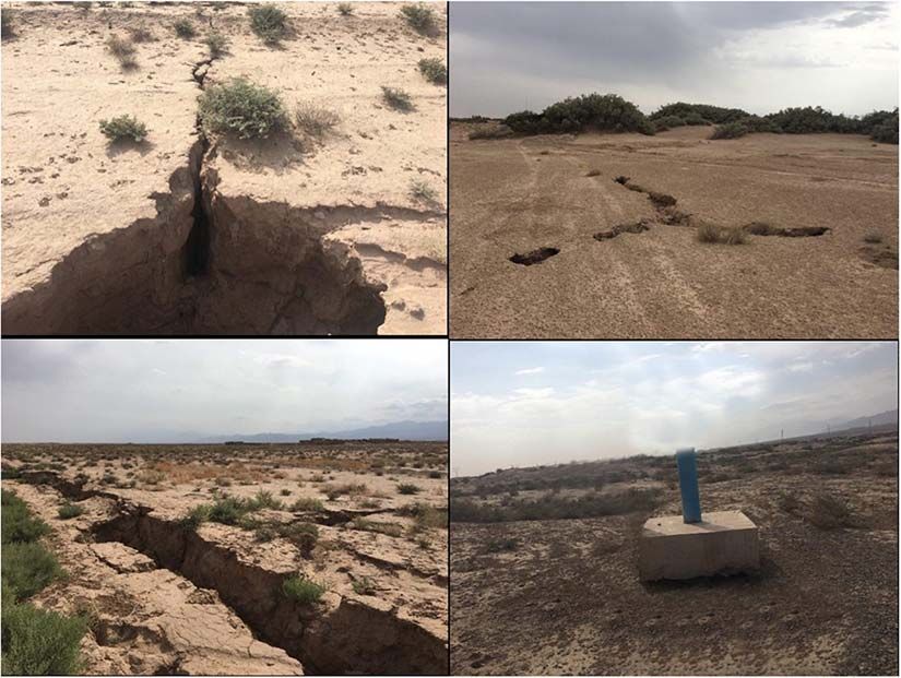
Arabameri et al.                                                                                          Performance Evaluation of GIS-Based Novel

A body of literature survey (Arabameri et al., 2020d, 2021;                 area has two classes of arid and hyper-arid. The minimum and
Babaee et al., 2020; Rezaei et al., 2020) and based on                      maximum temperature in this area is 16 and 22◦ C, respectively,
the local topographical, hydrological, climatological, geological           and also the minimum and maximum slopes in area are 0
and environmental condition, here we have selected twelve                   and 129%, respectively (Ghazifard et al., 2016; Goorabi et al.,
appropriate LS conditioning factors. Therefore, we used twelve              2020). Kashan plain is located in the foothills of the Karkas
geo-environmental conditioning factors namely elevation, aspect,            Mountains and on the margin of the central desert of Iran. Based
distance to road (DtR), groundwater drawdown, distance to                   on the land use map, poor rangeland the largest area (53.26%),
fault (DtF), topographic wetness index (TWI), distance from                 and then by agricultural (21.5%), barren land (16.19%) and the
stream (DtS), normalized differentiate vegetation index (NDVI),             remaining area is shared between afforest, sand dune, salt land
curvature, slope, land use and lithology to meet our objective.             and residential areas (Table 1). Based on the lithology map,
In this study, four popular MLAs namely the Maximum                         diverse lithological have covered the area in which the largest
Entropy (MaxEnt), general linear model (GLM), artificial neural             area pertains to the low level piedmont fan and valley terrace
network (ANN) and support vector machine (SVM) were                         deposits (68.33%), followed by unconsolidated windblown sand
used for modeling and mapping of LS, based on the state-                    deposits including sand dunes (18.83%) and the remaining area
of-the-art skillful characteristics and literature study (Abdollahi         is shared between other formations presented in detail in Table 1.
et al., 2019). The selection behind these MLAs are based on                 Based on the land type (geomorphology) map, plates the largest
their earlier involvement in different research work on natural             area (32.09%), and then by flood plain (26.98%), low land
hazard susceptibility studies and respective optimal prediction             (18.36%) and the remaining area is shared between mountains,
performance (Zamanirad et al., 2019; Mohebbi Tafreshi et al.,               scree and hill areas.
2020; Najafi et al., 2020). In the case of MaxEnt, it has the ability
to choose the correct estimation of the uncertain probability               Methodology
distribution and to select the highest entropy of the given                 The research work of the LSSM has been carried out in four
probabilistic constraints. The GLM algorithm is based on a                  steps (Figure 2).
logistic regression model and used for a fractional response
to handle a binary value dataset. Structured code input and                    • Preparing an LS inventory map using 239 LS points.
output nodes were determined by trial and error in ANN,                          Historical LS data were collected through field survey
and events and non-event phenomena were determined. SVM                          along with the help of Coppernnicus aerial view output
is mainly used for classification, error analysis; generalize the                and high resolution satellite images. A total of 12 geo-
overall function and find out about the two-class hyperplane in                  environmental control factors have been used to meet our
the dataset. Finally, a total of 11 ensembles, in which six are                  research objective.
two models ensemble and five are three-four models ensemble,                   • Multi-collinearity testing was conducted among the
have been developed for better predictive analysis of LSSM                       conditioning factors used in this study using inflation
in this region. A body of literature survey and best of our                      factor variance (VIF) and tolerance (TOL) techniques
knowledge it has been found that no research study on the                        (Band et al., 2020; Arabameri et al., 2021).
11 possible ensembles of aforementioned four ML algorithms                     • To map the LS susceptibility of a number of MLAs, i.e.,
were used in LS studies. The maximum ensemble methods were                       MaxEnt, GLM, ANN, and SVM have been used in this study
created using the aforementioned four popular ML algorithms                      together with a total of eleven ensemble methods.
to optimal estimation of LS prediction performance and this is                 • The performance of each model was validated by area under
the novelty in this research study. Thereafter, all of these output              curve (AUC) analysis.
results were validated by area under curve (AUC) analysis. As
a result, the LS susceptibility zones have been classified into             LS Inventory Map
five zones, i.e., very low, low, medium, high, and very high.               The LS Inventory Map (LSIM) is the primary mapping tool
Depending on the LS susceptibility zones, appropriate prevention            for LSSM. LSIM shows the spatial distribution of a number of
strategies should be taken to control future occurrences and                LS regions (Figure 1). It is well known that LS zones can be
proper management strategies.                                               predicted on the basis of both the historical and the current
                                                                            spatial distribution of LS. The current inventory map in this area
                                                                            has been prepared using RS-GIS technology. As a result, LS areas
MATERIALS AND METHODS                                                       have been identified from Coppernnicus aerial view output and
                                                                            extensive field surveys with the Global Positioning System (GPS)
Description of the Study Area                                               to locate the exact position in the field. In general, any type of
The Kashan plain is located in the North of the Esfahan Province            inventory map can be used to assess the relationship between
in the Kashan city (between 33◦ 400 0000 to 34◦ 350 0000 N, and             the distribution of a particular hazard location and the associated
51◦ 050 000 to 51◦ 550 0000 E) and covers about 2,231 km2 area              conditioning factors responsible for that hazard. A total of 239 LS
(Figure 1). Elevation in the study area ranges between 803 m                points were used in this study, in which 70% (167) was used as
and 1,671 m above mean sea level. The average annual rainfall               a training dataset and 30% (72) was used for dataset validation.
ranges between 75 and 185 mm and there is more rainfall                     In this study, we have followed the influence of data Splitting
in the west (Ghazifard et al., 2016). The climate of the study              performance (Nguyen et al., 2021) to divided the entire dataset

Frontiers in Earth Science | www.frontiersin.org                        3                                       May 2021 | Volume 9 | Article 663678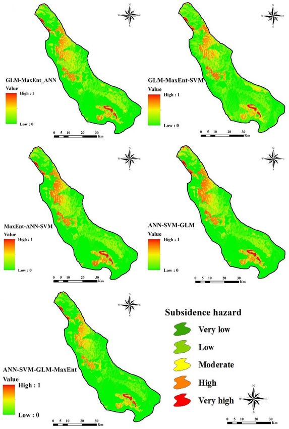
Arabameri et al.                                                                                                         Performance Evaluation of GIS-Based Novel

  FIGURE 1 | Location map of the study area.

TABLE 1 | Lithology of the study area.

Geo unit                                           Description                                                 Age                   Area (ha)           Area (%)

Qft2                             Low level piedmont fan and valley terrace deposits                         Quaternary              152464.36              68.34
OMq                  Limestone, marl, gypsiferous marl, sandy marl and sandstone (QOM FM)                Oligocene-Miocene           2337.61                1.05
Mur                  Red marl, gypsiferous marl, sandstone and conglomerate (Upper red Fm.)                  Miocene                 14054.89               6.3
Qft1                            High level piedmont fan and valley terrace deposits                         Quaternary               4826.55                2.16
Plc                                   Polymictic conglomerate and sandstone                                  Pliocene                3655.56                1.64
Qs,d                      Unconsolidated windblown sand deposit including sand dunes                        Quaternary               42023.55              18.84
Qcf                                                   Clay flat                                             Quaternary               3739.47                1.68

was splitting into 70:30 ratio. Some of the field photographs in                          into account for LSSM along with the geo-environmental
this study area are shown in Figure 3.                                                    conditions in this area. As already mentioned that in this
                                                                                          study we have selected a total of 12 suitable LSCFs based
                                                                                          on the literature survey and keeping in view the local geo-
Land Subsidence Conditioning Factors                                                      environmental conditions like topography, hydro-climatology
(LSCFs)                                                                                   and geological conditions. The 12 LSCFs used for this study
The quality of the predictive outcome of the LSSMs depends                                are elevation, aspect, distance to road (DtR), groundwater
to a large extent on the selection of control factors. The                                drawdown, distance to fault (DtF), topographic wetness index
evaluation of the relationship between the LS and their associated                        (TWI), distance from stream (DtS), normalized differentiate
conditioning factors is therefore very necessary as it influences                         vegetation index (NDVI), curvature, slope, land use and lithology
the modeling process. Twelve LSCFs have therefore been chosen                             (Figures 4A–L).
to prepare the LSSM for this area. There is no universal                                     Therefore, several data sources were used to prepare
criterion for the selection of these variables, although several                          these twelve conditioning factors. Different topographic and
literature studies have been conducted (Sahu et al., 2017).                               hydrological factors have been prepared from Advanced Land
The types of LS and the availability of data are also taken                               Observation satellite Phased Array type L-band Synthetic

Frontiers in Earth Science | www.frontiersin.org                                      4                                        May 2021 | Volume 9 | Article 663678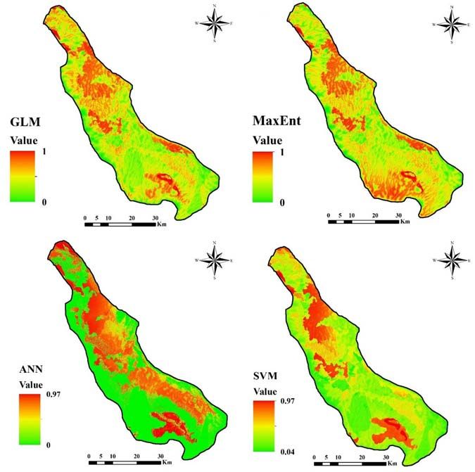
Arabameri et al.                                                                                          Performance Evaluation of GIS-Based Novel

     FIGURE 2 | Flowchart of research in this study area.

     FIGURE 3 | Some of mapped land subsidence in the study area.

Aperture Radar digital elevation model (ALOSPALSAR DEM)                     resolution of 10 m was used to prepare land use and NDVI map.
with a 12.5 m resolution which is freely available on the Alaska            Beside this, the topographic map was collected from National
Satellite Facility (ASF) website1 . Sentinel 2A satellite data with a       Geographic Organization of Iran2 at a scale of 1:1:50,000 to verify
1                                                                           2
    https://asf.alaska.edu/                                                     www.ngo-org.ir

Frontiers in Earth Science | www.frontiersin.org                        5                                       May 2021 | Volume 9 | Article 663678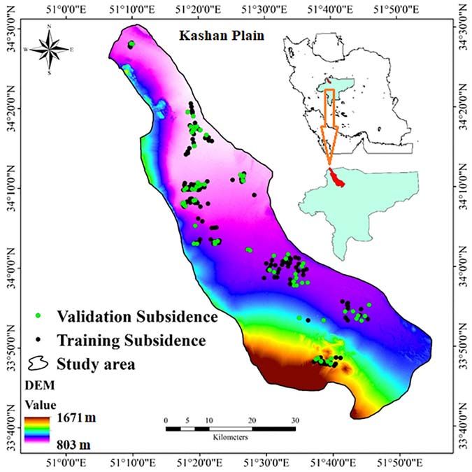
Arabameri et al.                                                                                                            Performance Evaluation of GIS-Based Novel

     FIGURE 4 | Land subsidence conditioning factors: (A) Elevation, (B) Aspect, (C) Distance to road, (D) Groundwater drawdown, (E) Distance from fault, (F) TWI,
     (G) Distance from stream, (H) NDVI, (I) Curvature, (J) Slope, (K) Lithology, and (L) Land use.

the land use map. The lithology map in this area was taken from                         803 to 1671 m (Figure 4A). The second side of the slope is
the Geological Maps of Iran collected from the Geological Society                       the derivative. Aspect is the altitude calculator and the slope
of Iran (GSI)3 at a scale of 1:100,000.                                                 direction of its eight neighbors. The aspect map of the present
    As a result, the elevation map was derived from the DEM                             study area (Figure 4B) has been shown. DtR is an important
analysis of the ArcGIS 10.5 platform, with values ranging from                          factor in the occurrence of LS due to surface pressure and may
                                                                                        cause LS in its surrounding area. The DtR range in this study
3
    http://www.gsi.ir/                                                                  ranges from 0 to 16,776 m (Figure 4C). Studies indicates that

Frontiers in Earth Science | www.frontiersin.org                                    6                                              May 2021 | Volume 9 | Article 663678
Arabameri et al.                                                                                                Performance Evaluation of GIS-Based Novel

several types of factors such as climate-hydrological and physical          natural hazard related susceptibility mapping and their optimal
factors significantly control soil moisture (Zhang et al., 2019).           prediction accuracy is based on suitable geo-environmental
   Among the various factors, groundwater depletion is the                  conditions (Arabameri et al., 2021). As a result, MC test has
most responsible conditioning factor for LS. The groundwater                been carried out in this study to analysis the specific relationship
map shows values from 1.8 to 21.1 m (Figure 4D). DtF is also                among all of these variables and minimize the bias. Generally,
responsible for the deformation of the soil surface through the             MC occurs when there is a high correlation among the two
use of LS. The value of a DtF map is between 0 and 16,679                   or more variables (Arabameri et al., 2017). In other words,
m (Figure 4E). The degree of water accumulation in the area                 MC test is required to ensure the independent conditioning
depends on the TWI, which is a secondary topographic variable.              factors in a dataset (Chen et al., 2020). Tolerance (TOL) and
The TWI map in this area was prepared using DEM on the                      variance inflation factors (VIF) techniques have been used by
ArcGIS 10.5 platform and the value ranges from 1.94 to 14.69                several researchers to test MC analyzes (Chowdhuri et al., 2020a).
(Figure 4F). The following equation has been used to calculate              Therefore, in this study, we also used these two techniques and
the TWI.                                                                  their respective equations were calculated as follows:
                                        As
                        TWI = log e                               (1)                                     TOL = 1 − R2j                                (3)
                                       tanβ

Where, As and β denotes cumulative catchment area (m2 ) and                                                           1
                                                                                                            VIF =                                      (4)
define slope angle, respectively.                                                                                    TOL
    The phenomenon of climate change and several human                      Where, R2j is the regression value of j variables in a dataset. The
induced activities are considered the two major drivers flow                MC occurred when the TOL value is < 0.10 or 0.20 and VIF value
pattern in a basin area and impacted on hydrological factors                is > 5 or 10 of a respective variables in a given dataset.
(Feng et al., 2020; Tian et al., 2020).
    DtS is also a significant factor for LS. The probability of LS          Modeling of LSSMs
is increasing away from the river, and vice versa. The DtS map
                                                                            Maximum Entropy (MaxEnt)
was shown in Figure 4G and ranged from 0 to 2,619 km. NDVI
                                                                            The MaxEnt algorithm is based on the principle of maximum
has the capacity to measure the growth and biomass of the
                                                                            entropy and is one of the most popular predictive machine
vegetation (Yilmaz, 2009). This factor also plays an important
                                                                            learning models (Woodbury et al., 1995). In general, MaxEnt
role in the LSSM, as land use largely affects the occurrence of LS.
                                                                            estimates the probability distribution of the target based on the
The NDVI value ranged from −0.72 to 0.82, with a lower value
                                                                            principle of maximum entropy and the probability distribution
indicating bare surface area and a higher value indicating forest
                                                                            of LS occurrences in this study. MaxEnt has always chosen the
cover (Figure 4H). The following equation was used to calculate
                                                                            highest entropy in a given probabilistic dataset. Apart from
the NDVI values using Sentinel 2A satellite data.
                                                                            this, the presence features are used only by the MaxEnt model
                                     Band8 − Band4                          and have a significant impact on inaccessible areas with a
                         NDVI =                                  (2)        reliable outcome (Reddy and Dávalos, 2003; Phillips et al., 2009).
                                     Band8 + Band4
                                                                            The relative influence of predictive variables (IPV) is estimated
Where, Band8 is near-infrared and Band4 is red reflectance of               using jackknife re-sampling techniques within this model to
the spectrum. Curvature represents the secondary geomorphic                 generate response curves. Model performance was calculated by
assets and shows the pattern of flow, sedimentation, erosion,               re-sampling the jackknife, excluding the predictor variables from
etc. (Yesilnacar, 2005). The curvature map in this study was                the data set (Yang et al., 2013). Basically, this model identifies
shown in Figure 4I and the values range from −4.77 to 5.66.                 the true distribution (π) of LS, i.e. target occurrences over area
The value of the slope map in this study area ranges from 0 to              X within a specific study area. Here, historical evidences of LS
129% (Figure 4J). LS is highly influenced by the slope of the area.         taken as a training dataset to define the true distribution (π). Let’s
Lithology is another key factor in the occurrence of LS as it affects       consider, the LS occurrence probability indicates the location of
the storage capacity of water. In this study, the lithological map          area X and the target probability distribution is π (X). Location
(Figure 4K) was classified into seven types. Table 1 shows details          X indicates the probability of LS occurring by P(y = 1|X) and the
of the lithological characteristics, such as their description, age
of formation, percentage area, etc. Finally, the land use map has
been prepared to understand the coverage of the surface area and            TABLE 2 | Land use classes in the study area.
its impact on the LS. The land use map (Figure 4L) for this area
                                                                            Land use                            Area (he)                        Area (%)
was classified into seven categories and their classes, along with
their respective areas, are shown in Table 2.                               Afforest                            10656.35                            4.78
                                                                            Agricultural                        47971.23                           21.50
Multi-Collinearity (MC) Analysis                                            Barren land                         36117.43                           16.19
MC can be defined as the linear relationship between two or more            Sand dune                           3277.57                             1.47
variables in the dataset (Alin, 2010). Linear dependency is the             Poor range                         118820.38                           53.26
top most priority given in this analysis and explained variables            Salt land                            613.01                             0.27
through correlation matrix (Saha et al., 2021b). Preparation of             Urban area                          5646.01                             2.53

Frontiers in Earth Science | www.frontiersin.org                        7                                              May 2021 | Volume 9 | Article 663678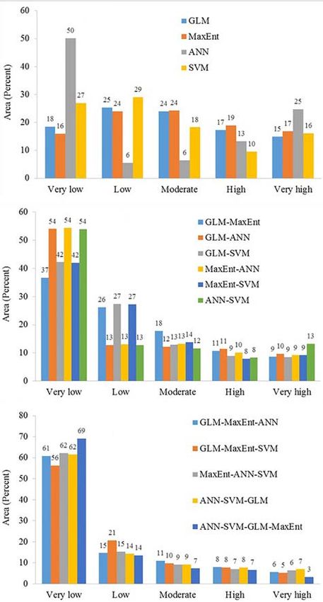
Arabameri et al.                                                                                               Performance Evaluation of GIS-Based Novel

Bayes rule has been applied to express this algorithm as follows:             Artificial Neural Network (ANN)
                                                                              One of the most popular MLAs, i.e., the ANN, is the most
                                                P y = 1 8(X)

                P y = 1 P(X|y = 1)                                           accurate and widely used forecasting model that has been
  P y=1 X =                                =                   (5)
                            P(X)                      1/|X|                   effectively applied in various areas of forecasting analysis, such
                                                                              as social, economic, stock issues, natural hazard susceptibility
Where, P y = 1 indicates success of LS occurrences and (X)

                                                                              mapping, etc. In general, ANN is a flexible statistical structure
indicates total number of occurrences over the whole study area.
                                                                              capable of identifying a non-linear relationship between input
π(X) is predicted through maximum entropy principle along
                                                                              and output variables of a dataset (Hsu et al., 1995). In modern
with Gibbs probability distribution. Thus, Gibbs probability
                                                                              times, this model has been used with the utmost precision
distribution may be expressed as follows:
                                                                              for forecasting, process control and pattern recognition in the
                                       n
                                                     !                        broader perspective of science and technology fields (Sudheer
                            1         X
                qλ (X) =         exp       λi fi (X)           (6)            et al., 2002). An ANN model has some unique features, and
                          Zλ (X)                                              the result of this model’s output forecast is more attractive
                                      i=1

                          X         X
                                                     !                        and accurate. The unique features of this model are based on
                 Zλ (X) =      exp      λi fi (x, y)           (7)            data-driven, self-adapted methods, the ability to generalize, and
                                    y          i                              the ability to manage complex non-linear relationships. Apart
                                                                              from that, among all non-linear classes, ANN is a universal
Where, Zλ (X) indicates normalization constant of a vector, λi                approximator capable of approximating complex class functions
indicates weights assigned of a vector. Furthermore, in the study             with high accuracy (Zhang and Qi, 2005). Among the various
area if m LS occurrences, variation between the regularization and            algorithms used in the ANN model, Multilayer Perceptron (MLP)
log likelihood is expressed as follows (Phillips and Dudík, 2008):            is the trendiest and widely used by a number of researchers
                                m                      n                      (Kosko, 1992). Therefore, within this MLP algorithm ANN model
                           1 X             X
                                                                              consists of three layers, i.e., input layer, hidden layer and output
               ψ (λ) =         In qλ (Xi ) −  βj λj                 (8)
                           m                                                  layer (Mandal and Mondal, 2019). If the function of the input
                               i=1                    j=1
                                                                              layer is not able to involve in a proper way than data structured
Where, βj represent the parameter of regularization for the jth               of the model is measured by hidden layer nodes (Arabameri
variables of predictor.                                                       et al., 2020c). The hidden layer is determined through trial and
                                                                              error method within this model (Gong et al., 1996). Thus, the
Generalized Linear Model (GLM)                                                model structure systematically predicts by input as well as hidden
The GLM was originally introduced and used by Nelder and                      layers and evaluates the output results. The output layer has been
Wedderburn (1972). In general, it is the probability of statistical           defined by Boolean value of 0 and 1. In this research study, 0
method with a logit function and widely used in the field                     indicates no LS and 1 indicates LS. According to Hagan et al.
of natural hazards analysis (Lucà et al., 2011). The simple                   (1995) the back propagation of an ANN model can be expressed
linear regression model was modified to form the GLM model.                   as follows:
One major advantages of this model is that its simplicity,                                                     p
                                                                                                              X
thus GLM extensively used in the wide fields of statistical                                          l
                                                                                                 net j (t) =     (yii−1 (t) wjil (t))         (10)
analysis (Vorpahl et al., 2012). The basic function of this model                                             i=o
is to develop multivariate regression between dependent and
independent variables. Basically, the extensive form of a simple              The net input of jth neuron of layer l and I iteration
linear regression model is therefore GLM’s ability to build up a                                                        (l )
non-normal distribution between datasets (Payne et al., 2012).                                         yjl (t) = f (net j (t)                        (11)
It also has the ability to develop binary datasets based on the                                                         1
presence and absence of data, using the logit link function                                           f (net) =                                      (12)
                                                                                                                    1 + e(−net)
for logistic regression. The GLM algorithm can easily handle
the binary data set with the fractional response of the logit                                          ej (t) = cj (t) − aj (t)                      (13)
link function (Garosi et al., 2018). The basic function of this
                                                                                                δlj (t) = elj (t) aj (t) 1 − aj x (t)

model fitting approaches includes finding out error distribution,                                                                                    (14)
determining the variables within this system and run the logit link
function. According to Bernknopf et al. (1988) the function of                δ factor for neuron jth in the output layer ith
GLM is as follows:                                                                                                   X l      (l+1)
                                                                                         δlj (t) = yjl (t) 1 − yj (t)  δj (t) wkj    (t)

                                                                                                                                                     (15)
                                        eC0 +C1 +X1 +···+Cn Xn
               Y = Pr y = 1 =                                       (9)
                                        1 + eC0 +C1 X1 +···+Cn Xn             δ factor for neuron jth in the hidden layer ith
Where, Y (logit-function) indicates the probability of an incident                                                 h                       i
happening and it varies from 0 to 1; X1 . . . Xn represent the                          wjil (t + 1) = wjil (t) + α wjil (t) − wjil (t − 1)
values of different controlling factors and C1 . . . Cn is their
                                                                                                            (l)    (l−1)
respective coefficient.                                                                                 + nδj (t) yj     (t)                         (16)

Frontiers in Earth Science | www.frontiersin.org                          8                                            May 2021 | Volume 9 | Article 663678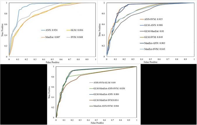
Arabameri et al. Performance Evaluation of GIS-Based Novel
Where, α is the momentum rate and n is the learning rate analysis (ROC-AUC) as it is a standard toll to do the same. ROC-
within this model. AUC is a statistical analysis and has been widely used by a number
of researchers to validate and assess the accuracy of several
Support Vector Machine (SVM) natural hazard susceptibility mappings (Moayedi et al., 2019;
The SVM is a supervised machine learning method and broadly Nguyen et al., 2019; Yuan and Moayedi, 2019; Zhang and Wang,
used in statistical test such as categorization and regression 2019). In general, it is a two-dimensional curve and consists of
analysis (Chen et al., 2017). The algorithm of SVM is based events and non-event phenomena (Frattini et al., 2010). It is a
on the principle of structural risk minimization and statistical graphical construction on X-axis known as sensitivity and Y-axis
learning (Vapnik, 2013). This model is binary classifiers and known as 1-speficity. The X and Y axis are false positive (FP) and
was introduced by Vapnik (2013) in 2013. In general, SVM true positive (TP), respectively. The four indices, i.e., true positive
has the capability of resolving the statistical dataset in the (TP), true negative (TN), false positive (FP) and false negative
way of classification and regression analysis. In SVM model (FN) have been used to assessment the ACC of ROC. In which,
errors are recognized through several classification functions true and false positive indicates LS and non-LS points correctly,
and finally generalize the overall function (Joachims, 1998). on the other side, true and false negative indicates LS and non-
The main two principles of SVM are the optimal hyper-plane LS points incorrectly. In the ROC-AUC sensitivity identifies LS
classification and the use of kernel function (Yao et al., 2008). and 1-specificity identifies non-LS accurately. The ROC-AUC
Therefore, the principle of hyper-plane is used to differentiate value ranges from 0.5 to 1. The lower value (0.5) indicates poor
into two classes, i.e., events and non-events, in this study it is performance and higher value (1) indicates good performance by
LS and non-LS. The situation of closeness of optimal hyper- the model. The following equations were used to calculate the
plane and training dataset is known as support vectors (Lee ROC-AUC value of a model.
et al., 2017). The statistical induced problems in a SVM model
TP
can be employed in two ways: optimal separating hyper-plane Sensitivity = (22)
from training dataset and conversion of non-linear data into TP + FN
linearly separable data through kernel function (Yao et al., 2008). TN
Specificity = (23)
In a SVM modeling, two classes have been created by hyper- FP + TN
plane, i.e., one is above the hyper-plane denoted by 1 and ( TP + TN)
P P
another is below the hyper-plane denoted by 0. The following AUC = (24)
(P + N)
equations have been used to calculate the hyper-plane in a SVM
model. Where, P indicates presence of LS and N indicates absence of LS.
n n n
X 1 XX
ϕi − ϕi ϕj yi yj xi , xj
Min (17) RESULTS
2
i=1 i=1 j=1
Subject to Multi-Collinearity Analysis
n
X The multi-collinearity analysis is the significant factor selection
Min ϕi yj = 0 and 0 ≤ αi ≤ D (18) method. It is the method where the land subsidence causative
i=1 factors (LSCFs) have been filtered from high correlations among
Where, x = xi , i = 1, 2,. . . n represent the input variables of vector, LSCF variables which have resulted in the erroneous output
y = yi , j = 1, 2,. . .n represent the output variables of vector and and uncertain predictions. In this study, the multi-collinearity
ϕi is Lagrange multipliers. analysis has been done through the Tolerance (TOL) and the
The decision function of SVM can be expressed as follows: Variance inflation factor (VIF) values of the LSCFs. When the
TOL value is below 0.1 and the VIF is above 5, it has a
X n problem with the multi-collinearity. Stream power index (SPI)
f (x) = sgn yi ϕi K xi , xj + a
(19) and drainage density followed the above rules and we removed
i=j the variables. Rests of the 12 variables have been considered as
LSCFs which have no multi-collinearity problems. The VIF of the
Where, a is the bias which indicate linear distance of hyper plane 12 LSCFs ranges from 2.864 to 1.085 and the TOL value ranges
from the origin, K xi , xj is kernel functions such as polynomial from 0.349 to 0.921 (Table 3).
(POL) and radial basis function (RBF) and, these can be expressed
as follow (Kavzoglu and Colkesen, 2009). Land Subsidence Susceptibility Maps
KPOL xi , xj = ( x ∗ y + 1)d
(20) (LSSMs)
2
The land subsidence susceptibility maps of the Kashan plain have
KRBF xi , xj = e−y||x−xi ||
(21) been created from the different single and ensemble classifier
machine learning (ML) models. Here, four-stage of machine
Validation and Accuracy Assessment learning land subsidence susceptibility models were used. First,
The Validation and evaluation of MLA and ensemble generated the four single or stand-alone ML; second, the two ensemble
LSSMs were done by using area under receiver operating curve models were created by the integrated of two single models;
Frontiers in Earth Science | www.frontiersin.org 9 May 2021 | Volume 9 | Article 663678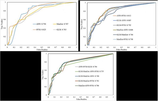
Arabameri et al. Performance Evaluation of GIS-Based Novel
FIGURE 5 | Land subsidence hazard mapping using: (A) GLM, (B) MaxEnt, (C) ANN, (D) SVM.
third, again three ensemble models were created by the integrated LSSMs were classified in five probability zones of very low, low,
of the three single ML models and last four ensemble models medium, high, and very high. There are many classification
were created by the integrated of the four single ML model. approaches to classify the land subsidence probability maps.
Each of the models has presented an LSSM (Figures 5–7). The These are natural break, quantile, equal interval, manual and
standard deviation. In this study, all the mentioned classification
methods have been applied and the natural break method
TABLE 3 | Multi-collinearity analysis of the subsidence factors. gave the best classification result for all the maps. Where
the spatial data have the big jump value, the natural break
Factors Collinearity classification scheme is suitable for classification probability
map (Ayalew and Yamagishi, 2005). The single ML and two,
Tolerance VIF
three, and four ensembles of LSSM have been analyzed in
Aspect 0.921 1.085 the next sections.
Elevation 0.492 2.031
Distance to road 0.611 1.621 LSSMs From Single ML Models
Groundwater withdraw 0.747 1.339 There are four single ML models have been used for the LSSM.
Distance to fault 0.801 1.248 The LSSMs of the GLM, MaxEnt, ANN, and SVM models have
Distance to stream 0.663 1.508 been presented in Figure 5 and indicate the same symbol for
Land use/land cover 0.617 1.620 each class. The areas of the very high, high, medium, low, and
Lithology 0.825 1.212 very low land subsidence susceptibility area in the GLM model
NDVI 0.770 1.299 are 15, 17, 24, 25, and 18% (Figure 8A). The percentage coverage
Curvature 0.871 1.112 of the very high, high, medium, low, and very low land subsidence
Slope 0.349 2.864 susceptibility area in the MaxEnt model are 17, 19, 24, 24, and 16.
TWI 0.416 2.403 The percent coverage of the very high, high, medium, low, and
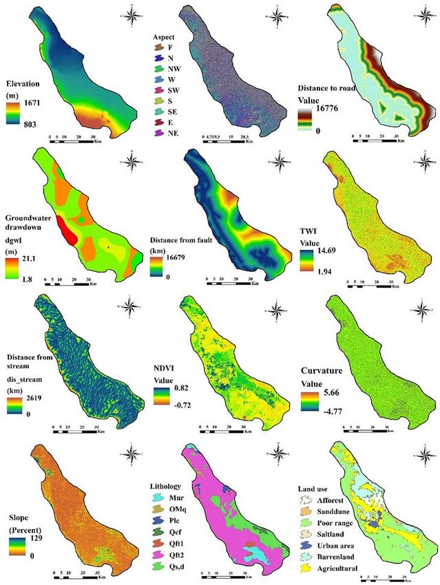
Frontiers in Earth Science | www.frontiersin.org 10 May 2021 | Volume 9 | Article 663678Arabameri et al. Performance Evaluation of GIS-Based Novel FIGURE 6 | Land subsidence hazard mapping using: (A) GLM-MaxEnt, (B) GLM-ANN, (C) GLM-SVM, (D) MaxEnt-ANN, (E) MaxEnt-SVM, (F) ANN-SVM. Frontiers in Earth Science | www.frontiersin.org 11 May 2021 | Volume 9 | Article 663678
Arabameri et al.                                                                                          Performance Evaluation of GIS-Based Novel

  FIGURE 7 | Land subsidence hazard mapping using: (A) GLM-MaxEnt-ANN, (B) GLM-MaxEnt-SVM, (C) MaxEnt-ANN-SVM, (D) ANN-SVM-GLM,
  (E) ANN-SVM-GLM-MaxEnt.

Frontiers in Earth Science | www.frontiersin.org                       12                                       May 2021 | Volume 9 | Article 663678
Arabameri et al.                                                                                                    Performance Evaluation of GIS-Based Novel

                                                                                       MaxEnt-ANN, MaxEnt-SVM, and ANN-SVM (Figure 6). The
                                                                                       very high probability of land subsidence areas varies from 9
                                                                                       to 10% in the above six ensemble models (Figure 8B). The
                                                                                       percentage of the high probability of land subsidence areas
                                                                                       ranges from 9 to 11. The percentage of medium probability
                                                                                       of land subsidence areas ranges from 12 to 18. The low and
                                                                                       very low probability area ranges from 13 to 27 and 37 to 54%,
                                                                                       respectively (Figure 8B). So the very high and high probabilities
                                                                                       of land subsidence classes have a good consistency in the six
                                                                                       ensemble models.

                                                                                       LSSMs From Second and Third Stage Ensemble
                                                                                       Models
                                                                                       In this stage, the possible ensemble models have been made by the
                                                                                       integration of three and four single ML models. These ensemble
                                                                                       models are GLM-MaxEnt-ANN, GLM-MaxEnt-SVM, MaxEnt-
                                                                                       ANN-SVM, and ANN-SVM-GLM-MaxEnt. The LSSMs were
                                                                                       prepared from these ensemble models presented in Figure 7.
                                                                                       In this second stage ensemble model, the percentage of very
                                                                                       high land subsidence susceptibility zone ranges from 5 to 6
                                                                                       (Figure 8C). The high land subsidence susceptibility probability
                                                                                       zone varies from 7 to 8%. The percentage of medium land
                                                                                       subsidence susceptibility probability zone ranges from 9 to
                                                                                       11. The low land subsidence probability zone varies from 15
                                                                                       to 21 and the very low land subsidence hazard probability
                                                                                       zone ranges from 56 to 69%. So there are no such differences
                                                                                       among the land subsidence hazard probability zone in second
                                                                                       stage ensemble models. The final ensemble model or the third
                                                                                       stage ensemble model was made through the integration of
                                                                                       all four single models. The final ensemble model has 3, 7,
                                                                                       7, 14, and 69% of land subsidence susceptible areas for the
                                                                                       very high, high, medium, low, and very low zone, respectively
                                                                                       (Figure 8C).

                                                                                       Evaluation of Land Subsidence Model
                                                                                       Validation is an important task for modeling based output
                                                                                       because of the accessibility of the model output determined
                                                                                       by the model output validation. The goodness of fit and
                                                                                       prediction accuracy of all ML ensemble models have been
  FIGURE 8 | Area percent classes in the different modeling: (A) one model, (B)
                                                                                       evaluated using training and validation land subsidence data
  two model, (C) three and four model.
                                                                                       applied the technique of area under curve (AUC) of the
                                                                                       receiver operating characteristic (ROC) curve. The evaluation
                                                                                       performance result of single ML and ensemble of two, three,
very low land subsidence susceptibility area in the ANN model                          and four ML models in training and validating stage have been
are 25, 13, 6, 6, and 50%. And the areas of very high to very                          shown in Figures 9, 10. All the single ML and ensemble two,
low land subsidence susceptibility area in the SVM model are                           three, and four ML methods showed the excellent goodness
16, 10, 18, 29, and 27%. The areas of probability classes of land                      of fit and prediction accuracy of the models. The AUC-ROC
subsidence in the models of GLM, MaxEnt, and SVM are almost                            of the single four ML model on the training stage showed
the same and they maintain consistency. The probability classes                        in Figure 9A. The ANN model has the highest AUC value
of LSSM in ANN model are slide difference from the other three                         (0.924) followed by SVM and GLM. On the validation stage
models (Figure 8A).                                                                    (Figure 10A), the SVM model got the highest (0.823) accuracy
                                                                                       among the single ML model and followed by ANN (0.794).
LSSMs From First Stage Ensemble Models                                                 In case of the ensemble of two ML methods (Figures 9B,
After the single ML land subsidence susceptibility model, the                          10B), the ensemble of the ANN-SVM model has higher AUC-
first stage ensemble models were created by the integrated of                          ROC in training (0.915) and validating (0.812) datasets and
two ML models. In this process, six ensemble models have                               followed by the GLM-ANN (0.808) and ANN-MaxEnt (0.805).
been created. These are GLM-MaxEnt, GLM-ANN, GLM-SVM,                                  The ensemble of three and four ML algorithms showed the

Frontiers in Earth Science | www.frontiersin.org                                  13                                      May 2021 | Volume 9 | Article 663678
Arabameri et al. Performance Evaluation of GIS-Based Novel FIGURE 9 | Area under the curves based on training datasets: (A) one model, (B) two model, (C) three and four model. FIGURE 10 | Area under the curves based on validation datasets: (A) one model, (B) two model, (C) three and four model. good accuracy of the model in both training and validating training and validating datasets. The result of the reliability of stage (Figures 9C, 10C). In the training stage, the highest AUC ML algorithms based on training datasets has depicted that the (0.89) value came from the ANN-SVM-GLM model followed ANN has the highest AUC (0.924) means this model is the by GLM-MaxEnt-ANN (0.884) and MaxEnt-SVM-ANN (0.884) best fit model for the land subsidence hazard mapping. And model. On the validating stage, the high prediction rate of the second and third best fit models are the ANN-SVM (0.915) AUC has come from GLM-MaxEnt-ANN (0.788) and followed and GLM-ANN (0.908). The prediction accuracy of the ML by MaxEnt-ANN-SVM (0.786). The AUC of the ensemble algorithms based on validating datasets showed the SVM has GLM-MaxEnt-ANN-SVM in training and validating stage are the highest AUC (0.823) followed by ANN-SVM (0.812) and 0.838 and 0.755. MaxEnt-ANN (0.808). The SVM model is the best model for the Table 4 shows the comparison of AUC-ROC for all single land subsidence susceptibility mapping because it has the finest ML and ensemble two, three, and four ML methods using prediction accuracy. Frontiers in Earth Science | www.frontiersin.org 14 May 2021 | Volume 9 | Article 663678
Arabameri et al.                                                                                                          Performance Evaluation of GIS-Based Novel

TABLE 4 | Area under the curve values of training and validation data in different models.

                                                                    AUC                                                        Prioritizing

Ro w                      Models                       Training             Validation            Priority based on training             Priority based on validation

1                           GLM                         0.816                 0.763                          12                                       14
2                         MaxEnt                        0.807                 0.767                          15                                       12
3                           ANN                         0.924                 0.794                           1                                       6
4                           SVM                         0.868                 0.823                           8                                       1
5                      GLM-MaxEnt                       0.81                  0.766                          14                                       13
6                        GLM-ANN                        0.908                 0.805                           3                                       4
7                        GLM-SVM                        0.849                 0.792                           9                                       7
8                      MaxEnt-ANN                       0.903                 0.808                           4                                       3
9                      MaxEnt-SVM                       0.843                 0.798                          10                                       5
10                       ANN-SVM                        0.915                 0.812                           2                                       2
11                   GLM-MaxEnt-ANN                     0.884                 0.788                           6                                       8
12                   GLM-MaxEnt-SVM                     0.814                 0.781                          13                                       11
13                  MaxEnt-ANN- S VM                    0.884                 0.786                           7                                       9
14                   ANN- S VM-GLM                      0.89                  0.784                           5                                       10
15                 GLM-MaxEnt-ANN-SVM                   0.838                 0.755                          11                                       15

DISCUSSION                                                                               models can give an optimal result and have controversy among
                                                                                         the researchers in this regards (Arabameri et al., 2020a). The
Several kinds of natural hazards related environment problems                            reliability and accurate result is the most predominate condition
has been solved by various research groups for sustainable                               for the LS hazard susceptibility mapping and researchers tried to
management and utilization of natural resources (Pradhan and                             form new novel ensemble models to produced good outcomes
Kim, 2017; Jiang et al., 2018; Tsai et al., 2019; Wang et al.,                           (Reichenbach et al., 2018). A lot of ML methods have been
2020; Xu et al., 2021) with the help of remote sensing (RS)                              applied in the previous past few years for the spatial probability
technology (Han et al., 2019; Hu et al., 2020; Zhang et al.,                             map of various kind of environmental hazards (Arabameri et al.,
2020c) and geographical information system (GIS) tool (Zuo                               2020c). The spatial analysis of LS indicates that subsidence
et al., 2015; Xu et al., 2018; Zhu et al., 2019; Yang et al., 2020b)                     specifically occurred in the flat areas particularly in the alluvial
and widespread progress in the computational facilities (Chao                            deposited land and agricultural areas located in arid regions
et al., 2018; Zhang et al., 2018, 2020b; Cao et al., 2020; Xu                            (Herrera-García et al., 2021). A present time, ML algorithms
et al., 2020; Feng et al., 2020). A noteworthy support from                              and their ensemble methods have been applied in various fields
the combination of RS and GIS technology gives efficiently                               for the susceptibility mapping and it has been shown to be
solution in the several types of natural hazards related problems                        effective in terms of predictive performance (Nguyen et al., 2019;
(Yang et al., 2018, 2020a; Zhang et al., 2019; Sun et al., 2021).                        Arabameri et al., 2020c; Feng et al., 2020; Liu et al., 2020; Zhang
Therefore, the geospatial technology, i.e., remote sensing and                           et al., 2020a; Saha et al., 2021b). Particularly, ensemble models
GIS has been providing high resolution multispectral satellite                           always enhanced the output result by integrated the several ML
data and their optimal processing which is immensely help to                             algorithms (Mojaddadi et al., 2017; Arabameri et al., 2020d;
analysis and solves several types of natural hazards related risk.                       Saha et al., 2021a).
The optimal data processing without any kinds of bias is done                                Thus, based on the literature survey and local geo-
through machine learning algorithms and their computation                                environmental conditions, different LSCFs have primarily
analysis has been presented through the help of GIS platform                             selected to perform the LSSM in this present study area.
(Pourghasemi and Rossi, 2017; Yang et al., 2015; Chen et al.,                            After that multi-collinearity assessment studies was carried
2019a; Zhu et al., 2019). Thus, in the present time, RS-GIS                              out and based on the result of multi-collinearity, a total
techniques and machine learning algorithms has been widely                               of 12 geo-environmental variables were selected for the LS
helped for optimal evaluation of many scientific problems (Yang                          susceptibility modeling (Chen et al., 2019b; Arabameri et al.,
et al., 2015; Wu et al., 2020).                                                          2020d). Thereafter, ML algorithms of GLM, MaxEnt, SVM, and
    Preparing of LS hazard susceptibility mapping is an important                        ANN were used and 11 possible ensemble models were developed
and one of the key challenging tasks among the land use planners                         to mapping LS susceptibility analysis. GLM or the logistic
(Arabameri et al., 2021). Therefore, several researchers proposed                        regression model is the most common statistical technique used
various kinds of models to address this key challenges and there                         for the prediction of landslide, flood, groundwater, gully erosion
has been great interest in improving the prediction performance                          susceptibility. The most advantages of GLM is that assumes a
of the hazards related susceptibility mapping through ML models                          linear relationship between a link function of the predictors
(Oh et al., 2019). It is also be mentioned here that no specific                         and response. The presence-only feature can be considered as

Frontiers in Earth Science | www.frontiersin.org                                    15                                            May 2021 | Volume 9 | Article 663678
Arabameri et al. Performance Evaluation of GIS-Based Novel advantages of MaxEnt because the determination of non-land CONCLUSION subsidence may result in uncertainty. SVM is a supervised based classification model and it is very capable of dealing The phenomenon of LS is one of the economic threats among with non-linear and high-dimensional grouping problems by the global people through the land degradation processes usually use of the different SVM based function (Huang and Zhao, induced by human misuse. Therefore, proper assessment and 2018). The ANN is an effective tool in a neural network, where management of this kind of natural hazard is crucial for the hidden and output layer nodes process their inputs (Lee sustainable development of any region. Hence, for the purpose et al., 2012) and successfully applied in this study. Ensemble of land management it is necessary to identification, modeling, models rapidly applied for the susceptibility modeling, but some assessment and analysis, and in the present research study it has author reported that ensemble models have better accuracy been carried out in the Kashan plain, Iran. Here, ML algorithms than the single models (Pham et al., 2019; Arabameri et al., of GLM, ANN, MaxEnt, SVM and their 11 possible ensemble 2020b; Chowdhuri et al., 2020b) consequently, some study classifier models were used for LS susceptibility modeling and reported that stand-alone ML models have better accuracy mapping. The final result indicates that the ANN model is the (Althuwaynee et al., 2014). best in training phase among the 15 models. But in the prediction In this study, we used a total of 15 models for land subsidence accuracy SVM model is the best among all models. Furthermore, modeling, but the ANN model was the best model by the success the consistency between the LSSMs was mentioned properly and rate of accuracy (AUC = 0.924) and the success rate AUC there are no such differences between the susceptibility zones. obtained from the training datasets. On the other hand, the Additionally, maximum ensemble models from the four ML SVM land subsidence hazard susceptibility model was the best models were developed in this study and in near future several model by the prediction accuracy rate (AUC = 0.823) and the others ML models can be used to compare and evaluate the predictive accuracy rate obtained from the validating datasets. An optimal result. Not only this, based on the optimal output of this ANN model is based on the non-linear statistical analysis of a study, these ensemble models can be used in further research given dataset and evaluation on the basis of observed coherence studies such as several environmental hazards potentiality network dynamics. Thus, ANN gives the highest accuracy in mapping and prediction. The best outcomes of the study are the training dataset. On the other side, SVM model try to land subsidence susceptibility maps which will help in the local relocate the idea based on the kernel function using unsupervised administrations and decision-makers in land use planning and function (Smits and Jordaan, 2002) and hence, gives the better proper management of land resources. As we know every research performance in validation dataset. The accuracy of the models study have some limitations, therefore this study also carried in success and prediction rate has been analyzed through the some limitation in terms of using limited LS causative factors and ROC- AUC curve. The ROC curve is a quantitative model lack of hydrological modeling. Another side, the strength of this evaluator successfully used for model performance evaluation in research study is the quality of the ML modeling and their optimal most of the studies (Su et al., 2017; Arabameri et al., 2020d). prediction result. The graphical presentation of the ROC- AUC curve created its most suitable model evaluator. The ROC- AUC curve result demonstrated that the 15 models performed well, but the SVM DATA AVAILABILITY STATEMENT and ANN-SVM models have made the best prediction of the gully erosion. Another study of LS in the Kashmar region, The original contributions presented in the study are included Iran based on MaxEnt models gives the result of ROC-AUC in the article/supplementary material, further inquiries can be is 88.9% (Rahmati et al., 2019a,b) which is significantly higher directed to the corresponding author/s. than the present study. Similarly, LS susceptibility studies in the Semnan province of Iran using ANN models gives the result of ROC-AUC is 0.919 (Arabameri et al., 2020d) which is less AUTHOR CONTRIBUTIONS than the our study result (AUC = 0.924). Therefore, studies indicate that the same ML models give different result in accuracy AA: conceptualization, methodology, software, validation, assessment from region to region, depending upon the local formal analysis, visualization, and resources. AA and SL geo-environmental factors. investigation. OA: data curation. AA and SL: writing—original Thus, in this study, the combination of remote sensing draft preparation. AA, SC, AS, IC, and HM: writing—review and and GIS techniques along with ML algorithms has given the editing. AA and SL: supervision. SL: funding. All authors have optimal result for land subsidence susceptibility mapping. read and agreed to the published version of the manuscript. Among the four ML algorithms, SVM gives the most optimal prediction performance outcome than the others. Therefore, based on the output maps of LS resulting FUNDING from hybrid ML algorithms will be very much helpful to the land use planners and policy makers for sustainable This research was supported by the Basic Research Project of the management and uses of land resources. The land degradation Korea Institute of Geoscience and Mineral Resources (KIGAM) process through LS is also control through taken proper and Project of Environmental Business Big Data Platform and management strategies. Center Construction funded by the Ministry of Science and ICT. Frontiers in Earth Science | www.frontiersin.org 16 May 2021 | Volume 9 | Article 663678
Arabameri et al.                                                                                                                        Performance Evaluation of GIS-Based Novel

REFERENCES                                                                                          for modeling landslide susceptibility. Catena 172, 212–231. doi: 10.1016/j.
                                                                                                    catena.2018.08.025
Abdollahi, S., Pourghasemi, H. R., Ghanbarian, G. A., and Safaeian, R. (2019).                   Chen, W., Shahabi, H., Shirzadi, A., Hong, H., Akgun, A., Tian, Y., et al.
   Prioritization of effective factors in the occurrence of land subsidence and                     (2019b). Novel hybrid artificial intelligence approach of bivariate statistical-
   its susceptibility mapping using an SVM model and their different kernel                         methods-based kernel logistic regression classifier for landslide susceptibility
   functions. Bull. Eng. Geol. Environ. 78, 4017–4034. doi: 10.1007/s10064-018-                     modeling. Bull. Eng. Geol. Environ. 78, 4397–4419. doi: 10.1007/s10064-018-
   1403-6                                                                                           1401-8
Alin, A. (2010). Multicollinearity. WIREs Comput. Stat. 2, 370–374. doi: 10.1002/                Chen, W., Xie, X., Wang, J., Pradhan, B., Hong, H., Bui, D. T., et al. (2017). A
   wics.84                                                                                          comparative study of logistic model tree, random forest, and classification and
Althuwaynee, O. F., Pradhan, B., Park, H.-J., and Lee, J. H. (2014). A novel                        regression tree models for spatial prediction of landslide susceptibility. Catena
   ensemble bivariate statistical evidential belief function with knowledge-based                   151, 147–160. doi: 10.1016/j.catena.2016.11.032
   analytical hierarchy process and multivariate statistical logistic regression for             Chowdhuri, I., Pal, S., Arabameri, A., Ngo, P., Chakrabortty, R., Malik, S., et al.
   landslide susceptibility mapping. Catena 114, 21–36. doi: 10.1016/j.catena.2013.                 (2020a). Ensemble approach to develop landslide susceptibility map in landslide
   10.011                                                                                           dominated Sikkim Himalayan region, India. Environ. Earth Sci. 79, 1–28. doi:
Arabameri, A., Asadi Nalivan, O., Chandra Pal, S., Chakrabortty, R., Saha, A.,                      10.1007/s12665-020-09227-5
   Lee, S., et al. (2020a). Novel machine learning approaches for modelling                      Chowdhuri, I., Pal, S. C., and Chakrabortty, R. (2020b). Flood susceptibility
   the gully erosion susceptibility. Remote Sens. 12:2833. doi: 10.3390/rs1217                      mapping by ensemble evidential belief function and binomial logistic regression
   2833                                                                                             model on river basin of eastern India. Adv. Space Res. 65, 1466–1489. doi:
Arabameri, A., Asadi Nalivan, O., Saha, S., Roy, J., Pradhan, B., Tiefenbacher, J. P.,              10.1016/j.asr.2019.12.003
   et al. (2020b). Novel ensemble approaches of machine learning techniques in                   Cigna, F., and Tapete, D. (2021). Present-day land subsidence rates, surface faulting
   modeling the gully erosion susceptibility. Remote Sens. 12:1890. doi: 10.3390/                   hazard and risk in Mexico City with 2014–2020 Sentinel-1 IW InSAR. Remote
   rs12111890                                                                                       Sens. Environ. 253:112161. doi: 10.1016/j.rse.2020.112161
Arabameri, A., Pourghasemi, H. R., and Yamani, M. (2017). Applying different                     Erkens, G., and Stouthamer, E. (2020). The 6M approach to land subsidence. Proc.
   scenarios for landslide spatial modeling using computational intelligence                        Int. Assoc. Hydrol. Sci. 382, 733–740. doi: 10.5194/piahs-382-733-2020
   methods. Environ. Earth Sci. 76:832.                                                          Famiglietti, J. S. (2014). The global groundwater crisis. Nat. Clim. Change 4,
Arabameri, A., Saha, S., Roy, J., Chen, W., Blaschke, T., and Tien Bui, D. (2020c).                 945–948. doi: 10.1038/nclimate2425
   Landslide susceptibility evaluation and management using different machine                    Feng, W., Lu, H., Yao, T., and Yu, Q. (2020). Drought characteristics and its
   learning methods in The Gallicash River Watershed, Iran. Remote Sens. 12:475.                    elevation dependence in the Qinghai–Tibet plateau during the last half-century.
   doi: 10.3390/rs12030475                                                                          Sci. Rep. 10, 1–11.
Arabameri, A., Saha, S., Roy, J., Tiefenbacher, J. P., Cerda, A., Biggs, T., et al.              Frattini, P., Crosta, G., and Carrara, A. (2010). Techniques for evaluating the
   (2020d). . A novel ensemble computational intelligence approach for the spatial                  performance of landslide susceptibility models. Eng. Geol. 111, 62–72. doi:
   prediction of land subsidence susceptibility. Sci. Total Environ. 26:138595. doi:                10.1016/j.enggeo.2009.12.004
   10.1016/j.scitotenv.2020.138595                                                               Galloway, D. L., and Burbey, T. J. (2011). Review: regional land subsidence
Arabameri, A., Yariyan, P., and Santosh, M. (2021). Land subsidence spatial                         accompanying groundwater extraction. Hydrogeol. J. 19, 1459–1486. doi: 10.
   modeling and assessment of the contribution of geo-environmental factors to                      1007/s10040-011-0775-5
   land subsidence: comparison of different novel ensemble modeling approaches.                  Garosi, Y., Sheklabadi, M., Pourghasemi, H. R., Besalatpour, A. A., Conoscenti, C.,
   Res. Sq. [Preprint]. doi: 10.21203/rs.3.rs-194202/v1                                             and Van Oost, K. (2018). Comparison of differences in resolution and sources
Ayalew, L., and Yamagishi, H. (2005). The application of GIS-based logistic                         of controlling factors for gully erosion susceptibility mapping. Geoderma 330,
   regression for landslide susceptibility mapping in the Kakuda-Yahiko                             65–78. doi: 10.1016/j.geoderma.2018.05.027
   Mountains, Central Japan. Geomorphology 65, 15–31. doi: 10.1016/j.geomorph.                   Ghazifard, A., Moslehi, A., Safaei, H., and Roostaei, M. (2016). Effects of
   2004.06.010                                                                                      groundwater withdrawal on land subsidence in Kashan Plain, Iran. Bull. Eng.
Babaee, S., Mousavi, Z., Masoumi, Z., Malekshah, A. H., Roostaei, M., and                           Geol. Environ. 75, 1157–1168. doi: 10.1007/s10064-016-0885-3
   Aflaki, M. (2020). Land subsidence from interferometric SAR and groundwater                   Ghorbanzadeh, O., Rostamzadeh, H., Blaschke, T., Gholaminia, K., and Aryal,
   patterns in the Qazvin plain, Iran. Int. J. Remote Sens. 41, 4780–4798. doi:                     J. (2018). A new GIS-based data mining technique using an adaptive neuro-
   10.1080/01431161.2020.1724345                                                                    fuzzy inference system (ANFIS) and k-fold cross-validation approach for land
Band, S. S., Janizadeh, S., Chandra Pal, S., Saha, A., Chakrabortty, R., Shokri,                    subsidence susceptibility mapping. Nat. Hazards 94, 497–517. doi: 10.1007/
   M., et al. (2020). Novel ensemble approach of deep learning neural network                       s11069-018-3449-y
   (DLNN) model and particle swarm optimization (PSO) algorithm for                              Gong, P., Pu, R., and Chen, J. (1996). Elevation and forest-cover data using neural
   prediction of gully erosion susceptibility. Sensors 20:5609. doi: 10.3390/                       networks. Photogr. Eng. Remote Sens. 62, 1249–1260.
   s20195609                                                                                     Goorabi, A., Karimi, M., Yamani, M., and Perissin, D. (2020). Land
Bernknopf, R. L., Campbell, R. H., Brookshire, D. S., and Shapiro, C. D. (1988).                    subsidence in Isfahan metropolitan and its relationship with geological
   A probabilistic approach to landslide hazard mapping in Cincinnati, Ohio,                        and geomorphological settings revealed by Sentinel-1A InSAR
   with applications for economic evaluation. Bull. Assoc. Eng. Geol. 25, 39–56.                    observations. J. Arid Environ. 181:104238. doi: 10.1016/j.jaridenv.2020.10
   doi: 10.2113/gseegeosci.xxv.1.39                                                                 4238
Cao, B., Wang, X., Zhang, W., Song, H., and Lv, Z. (2020). A many-objective                      Guzy, A., and Malinowska, A. A. (2020). State of the art and recent advancements
   optimization model of industrial internet of things based on private blockchain.                 in the modelling of land subsidence induced by groundwater withdrawal. Water
   IEEE Netw. 34, 78–83. doi: 10.1109/mnet.011.1900536                                              12:2051. doi: 10.3390/w12072051
Chao, L., Zhang, K., Li, Z., Zhu, Y., Wang, J., and Yu, Z. (2018).                               Hagan, M. T., Demuth, H. B., and Beale, M. H. (1995). Neural Network Design
   Geographically weighted regression based methods for merging satellite and                       (Electrical Engineering). Belmont, CA: Thomson Learning.
   gauge precipitation. J. Hydrol. 558, 275–289. doi: 10.1016/j.jhydrol.2018.                    Han, C., Zhang, B., Chen, H., Wei, Z., and Liu, Y. (2019). Spatially distributed
   01.042                                                                                           crop model based on remote sensing. Agric. Water Manag. 218, 165–173. doi:
Chen, W., Fan, L., Li, C., and Pham, B. T. (2020). Spatial prediction of landslides                 10.1016/j.agwat.2019.03.035
   using hybrid integration of artificial intelligence algorithms with frequency                 Herrera-García, G., Ezquerro, P., Tomás, R., Béjar-Pizarro, M., López-Vinielles, J.,
   ratio and index of entropy in Nanzheng County, China. Appl. Sci. 10:29. doi:                     Rossi, M., et al. (2021). Mapping the global threat of land subsidence. Science
   10.3390/app10010029                                                                              371, 34–36. doi: 10.1126/science.abb8549
Chen, W., Panahi, M., Tsangaratos, P., Shahabi, H., Ilia, I., Panahi, S., et al. (2019a).        Hsu, K., Gupta, H. V., and Sorooshian, S. (1995). Artificial neural network
   Applying population-based evolutionary algorithms and a neuro-fuzzy system                       modeling of the rainfall-runoff process. Water Resour. Res. 31, 2517–2530.

Frontiers in Earth Science | www.frontiersin.org                                            17                                                 May 2021 | Volume 9 | Article 663678
You can also read