Site suitability analysis for potential agricultural land with spatial fuzzy multi criteria decision analysis in regional scale under semi arid ...
←
→
Page content transcription
If your browser does not render page correctly, please read the page content below
www.nature.com/scientificreports
OPEN Site suitability analysis
for potential agricultural land
with spatial fuzzy multi‑criteria
decision analysis in regional
scale under semi‑arid terrestrial
ecosystem
Barış Özkan1, Orhan Dengiz2* & İnci Demirağ Turan3
The main purpose of this study is to identify suitable potential areas for agricultural activities in
the semi-arid terrestrial ecosystem in the Central Anatolia Region. MCDA was performed in fuzzy
environment integrated with GIS techniques and different geostatistical interpolation models,
which was chosen as the basis for the present study. A total of nine criteria were used, as four terrain
properties and five soil features to identify potential sites suitable for agriculture lands in Central
Anatolia which covers approximately 195,012.7 km2. In order to assign weighting value for each
criterion, FAHP approach was used to make sufficiently sensitive levels of importance of the criteria.
DEM with 10 m pixel resolution used to determine the height and slope characteristics, digital geology
and soil maps, CORINE land use/land cover, long-term meteorological data, and 4517 soil samples
taken from the study area were used. It was identified that approximately 30.7% of the total area
(59,921.8 ha) is very suitable and suitable for potential agriculture activities on S1 and S2 levels, 42.7%
of the area is not suitable for agricultural uses, and only 27% of the area is marginally suitable for
agricultural activities. Besides, it was identified that 34.8% of the area is slightly suitable.
Lands are one of the most important wealth of countries. Their quality and quantity are directly related to
agricultural development and food safety. Therefore, sustainable agricultural production is the most important
goal of developed or developing countries’ agricultural policies. On the other hand, the pressure on the lands
is increasing day by day with the increasing population. Particularly, the socio-economic needs of the rapidly
growing population in developing countries forced the allocation of land resources for different uses for food
production as the main goal. Therefore, the basis of the socio-economic development of countries depends on
the abundance of natural resources and policies of using these resources. In addition, the pressure of growing
population and competition arising from differences in land use requires more efficient land use and manage-
ment. Rational and sustainable land use is an important issue for the benefit of the present and future population
for land users and decision makers interested in the conservation of land resources. However, especially fertile
farmlands have been negatively affected under the influence of industrialization, urbanization and wrong land
use. Also, these fertile farmlands are exposed to excessive fertilization, disinfestation, domestic and industrial
wastes. This pressure on soils leads to irreversible consequences.
Amount of arable land in the Turkey was about 27.5 million ha in the ‘80 s. According to the data of recent
years, approximately 31% of the total land area of 78 million hectares in Turkey, i.e., approximately 24 million ha
is considered as agricultural land1. Turkey has been faced the risk of land degradation and inappropriate use due
to natural (i.e. climatic, topographic) and anthropogenic conditions. Especially the loss of agricultural land by
erosion causes irreversible consequences. This case has been particularly felt in the Central Anatolia Region. This
1
Department of Industrial Engineering, Faculty of Engineering, Ondokuz Mayıs University, 55139 Samsun,
Turkey. 2Department of Soil Science and Plant Nutrition, Faculty of Agriculture, Ondokuz Mayıs University,
55139 Samsun, Turkey. 3Department of Geography, Faculty of Economic, Administrative and Social Sciences,
Samsun University, 55139 Samsun, Turkey. *email: dengizorhan@gmail.com
Scientific Reports | (2020) 10:22074 | https://doi.org/10.1038/s41598-020-79105-4 1
Vol.:(0123456789)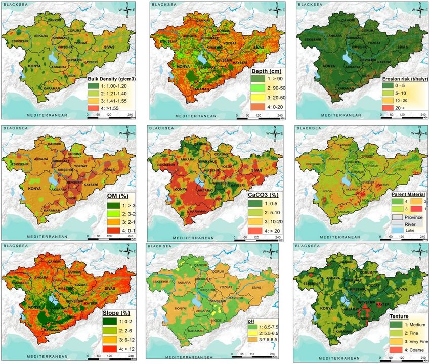
www.nature.com/scientificreports/
is why, identification of climate, vegetation, soil, and topographic features to make the most suitable decisions on
land use and identification of suitable areas for cultivation land to reveal the correct uses by making comparisons
between different lands, land evaluation and land use planning studies are quite important.
Identifying the suitability and quality of the lands has great importance for deciding on the use of land
according to its potential and protecting natural resources for future generations. In this case, especially poten-
tial agricultural land should be identified and land use planning should be performed to make rational analysis
and evaluation of fast, accurate, sufficient information and data about soil and land resources by using today’s
technologies2.
The development of methodologies facilitating the quantification of land suitability has been the main objec-
tive of the studies assessing the land evaluation3–5. In general, land evaluation methods are divided into two as
qualitative methods based on expert knowledge and quantitative models based on simulation m odels6. Quanti-
tative models are highly detailed for land performance and they often require much data, time and cost. On the
other hand, land and soil features in the identification of agricultural land suitability in qualitative approaches
are expressed in mathematical formulas. In this context, the evaluation of land suitability for agricultural activi-
ties is naturally regarded as a complex problem with multiple criteria. In other words, an evaluation approach
involving multiple criteria would be more appropriate for land evaluation analysis studies. Today, besides the
current techniques such as remote sensing and Geographic Information Systems (GIS), these challenges can
be overcome by using approaches such as Multi-Criteria Decision Analysis (MCDA) to make rational analyses
and evaluations7–12. Analytic Hierarchy P rocess13 (AHP) assigning weights to evaluation criteria belongs to often
used MCDA methods. AHP is capable of identifying and incorporating inconsistencies in decision-making14.
Typically, a priority vector is calculated based on the pair-wise comparison rising from a value determined by
experts on a 1–9 scale. On the other hand, setting the explicit numerical values to evaluation criteria may be
difficult or imprecise15 in reality. As a result, the evaluation criteria usually cannot be assigned precisely and
decision makers indicate their weights in linguistic t erms16. Applying fuzzy logic accommodates a mathemati-
cal strength to cover the uncertainties related to human cognitive p rocess17. Buckley (1985)18 integrates fuzzy
sets with AHP for uncertainty contemplation. Moreover, this approach has been used for different problems,
including prioritization of dimensions of visual m erchandising19, assessment of mine security r isk20, assessment
of surface water q uality21, evaluation of occupational s tress22, location selection of chromite processing p lant23,
24 25
selection of optimum maintenance s trategy , and ranking of geological risks .
Identification of potential land suitability classes in the MCDA approach is usually developed using a four-
stage process. These stages are (i) indicator selection, (ii) indicator categorization and scoring, (iii) weighting the
indicators according to their significance, and (iv) calculating the scores according to a selected model5,12,26,27.
However, the developed land quality indexes generally applicable under certain purposes and environmental
conditions on a limited scale28. Therefore, no land quality index can be used universally and suitable for all
kinds of geography29. Hence, indices that can identify the land quality of land and soil properties, usage type and
plant species for all geographies cannot be expected 30,31. Also, the development of a model that can represent
all ecological variables and socio-cultural habits is not practically possible and in theory, it is not economical in
terms of time, labour and c ost32.
In this study, it is aimed to identify the potential areas suitable for agricultural activities by taking into the
MCDA approach in the Fuzzy Analytic Hierarchy Process (FAHP) environment in Central Anatolia Region
that has a semi-arid terrestrial ecosystem. In addition, the fundamental basis hypothesis of this study is not only
assisting to identify lands suitable for agricultural applications but also it is aimed to assist sustainable use and
management of lands by taking into consideration the characteristics of soils, which are the most important
sensitive elements of arid and semiarid terrestrial ecosystem against to land degradation and desertification.
Materials and methods
Field description of the study area. The study area is between 30° 01′ 07″ and 38° 43′ 19″ east lon-
gitudes and 36° 18′ 08″ and 41° 07′ 11″ north latitudes and has a surface area of approximately 195,013 km2
(Fig. 1). The study area is within the borders of Bolu, Karabük, Çankırı, Çorum, Kırıkkale, Ankara, Eskişehir,
Yozgat, Kırşehir, Aksaray, Konya, Niğde, Kayseri, Sivas, and Karaman provinces. The elevation of the study area
is between 1600 and 3800 m above sea level. The region has an average elevation of 1200 m.
With an average slope of 9.6%, Central Anatolia Region is generally composed of flat fields and volcanic
mountains rising in these fields. The area around Lake Tuz and Konya province have large flat fields. However,
slope exceeds 30% towards the southeast and north of the study area, which is regarded as very steep. Also, 36.4%
of the Central Anatolia Region is distributed in the southeast, south, and southwest aspect while, 38.1% is located
in the north, northeast and northwest (Fig. 2).
The geological material of the Central Anatolia Region is composed of metamorphic, granitic and ophiolitic
units, and this is regarded as Central Anatolian Crystalline Complex. The sedimentary origin main rock units
of the Central Anatolian Crystalline Complex composed of Precambrian and early Paleozoic meta-clastic and
meta-magmatic rocks (para-orthogneiss and rare carbonate arabantic schists) at the bottom, and late Paleozoic
and Mesozoic meta-clastic rocks, calc-schist and marbles at the top. Non-metamorphic Upper-Maastrichtian-
Lower Paleocene cover units on top of these units are covered by Paleocene-Eocene volcanic, volcaniclastic
and carbonate rocks, Oligocene–Miocene evaporites, continental clastics with volcaniclastic and volcanic rocks
represent the younger cover units of the Central Anatolian Crystalline C omplex33.
The humid air of the seas cannot easily penetrate the Central Anatolia Region due to it is surrounded by high
mountains. Therefore, the region is dominated by terrestrial climatic conditions where summers are usually hot
and dry in summers and winters are cold and snowy. The degree of terrestrial climate increases towards the east
with increasing altitude in the region. In this context, it can be said that semi-continental and semi-arid climatic
Scientific Reports | (2020) 10:22074 | https://doi.org/10.1038/s41598-020-79105-4 2
Vol:.(1234567890)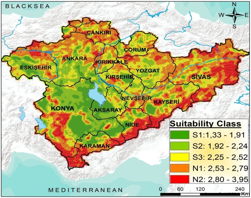
www.nature.com/scientificreports/
Figure 1. Location map of the study area (the map was created by the authors using the ArcGIS 10.2, http://
esri.com).
conditions are more effective in the Central Anatolia Region. While the average annual temperature ranges from
8 °C to 12 °C at 0–1500 m elevations, it is well-known that the average temperature falls below 4 °C in higher
elevations, such as Mount Erciyes. Central Anatolia Region is the region with the least rainfall in Turkey (Konya
326 mm, Karapınar 250 mm, Kayseri 375 mm, Kırşehir 378 mm, Çankırı 400 mm). The most rainfall occurs
during the spring season in the east of the region and during the winter season in the west of the region. It can be
said that semi-arid climatic conditions dominate most of the region when rainfall efficiency is considered. While
the average annual relative humidity in the central part of Central Anatolia is around 55–60%, there are areas
where relative humidity rises to 60–65% due to an increase in elevation and a decrease in air temperature. The
relative humidity, which is reaching up to 80% in the winter season, is around 40–50% in summer. In addition
to this, in summer some days, especially in August, the relative humidity in the air decreases up to 2%, which
increases the evaporation extremely34.
The low biomass in grass (steppe) vegetation due to drought and terrestrial conditions that dominate the
summer seasons in the lower elevations of the Central Anatolia Region caused the soil to be poor in organic
substances. Sparse and arid forests are available, where oaks dominate the bottom part and black pines dominate
the top part, in areas up to 2000 m starting over the steppes in Central Anatolia Region. However, anthropogenic
steppes have become dominant since most of these forests have been d estroyed35. According to ecological condi-
tions in Central Anatolia, steppe fields are available in the area starting from Konya-Eregli plains in the south
and extending to the Eskişehir Plain along the Sakarya and Porsuk brooks from the northwest of Lake Tuz36.
The dominant species that make up the steppe vegetation in Central Anatolia are; Artemisia fragrans, Thymus
squarrosus, Festuca valesiaca, Ambyliopyrum muticum, Agropyron divaricatum, Hordeum murinum, Onopordon
acanthium, Satureja cuneifolia, Stipa sp., Bromus sp., Festuca sp., Alyssum sp., Ajuga sp., Centaurea sp., Galium sp.,
Medicago sp., Marrubium sp., Nigella sp., Papaver sp., Convolvulus sp., Crucianella sp., Trifolium sp., Salvia sp.,
Senecio sp., Sideritis sp., Ziziphora sp., Leontodon asperrimum’dur. Başlıca çalılar ise; Prunus spinosa, Jasminum
fruticans, Rosa sulphurea, Crataegus orientalis, Lonicera etrusca, and Clematis vitalba36. According to the Central
Anatolia Region CORINE-2012 land use-land cover classification, 40% of the area is agricultural area and this
is followed by pasture area with 35.7% and forests with %14.5 (Fig. 2).
Soil sampling and soil physico‑chemical analyses. Total 4517 coordinated soil samples were taken
from a depth of 0–30 cm from the study area (Fig. 3). Samples brought to the laboratory are prepared for physical
and chemical analysis after the separation from roots and coarse particles. Soil properties were determined with
the following methods: soil particle size distribution by the hydrometer method; pH and electrical conductivity
(EC) in 1:2.5 (w/v) in soil/water suspension by pH-meter and EC-meter, respectively; C aCO3 content by the
volumetric method37. All soil samples were sieved through a 150 μm mesh before determination of the total
organic matter content with the wet oxidation (Walkley-Black) method with K 2Cr2O738.
Interpolation analyses and descriptive statistics. In this study, different interpolation methods
(Inverse Distance Weighing-IDW with the weights of 1, 2, 3 and radial basis function-RBF with thin plate spline
(TPS), simple kriging (OK) with spherical, exponential and gaussian variograms, ordinary kriging (OK) with
spherical, exponential and gaussian variograms, universal kriging (OK) with spherical, exponential and gauss-
Scientific Reports | (2020) 10:22074 | https://doi.org/10.1038/s41598-020-79105-4 3
Vol.:(0123456789)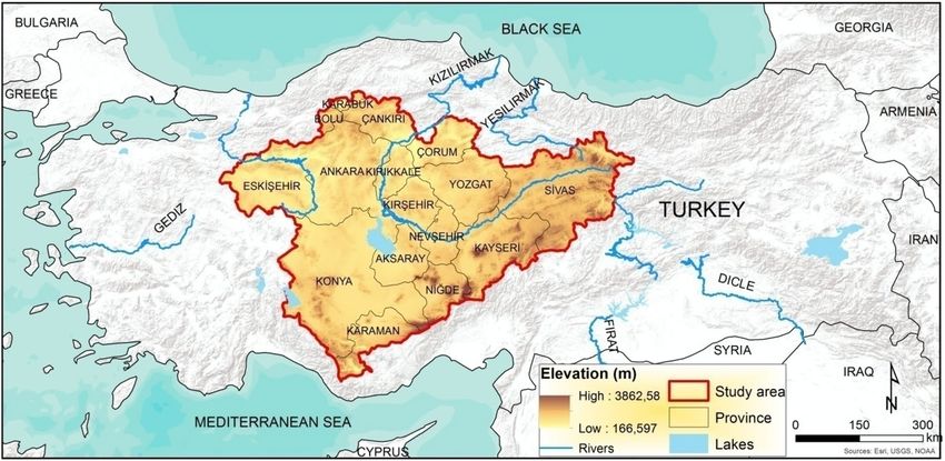
www.nature.com/scientificreports/
Figure 2. Elevation, slope, aspect and land cover-land use maps of the Central Anatolia Region (the maps were
created by the authors using the ArcGIS 10.2, http://esri.com).
ian variograms) were applied for predicting the spatial distribution of soil some parameters texture, pH, bulk
density, lime and organic matter content) with ArcGIS 10.2.2v.
In the present study, root mean square error (RMSE) was used to assess and figure out the most suitable
interpolation model. That’s why, the lowest RMSE indicates the most accurate prediction. Estimates are deter-
mined by using Eq. (1).
(zi∗ − zi )2
RMSE = (1)
n
where; RMSE: root mean square error, Zi is the predicted value, Zi* is the observed value, and n is the number
of observations.
Descriptive statistics as minimum, maximum, mean, standard deviation, skewness, kurtosis coefficient and
coefficients of variation of physico-chemical properties of surface soil samples were calculated.
Multi criteria assessment approach. The selection of indicators to be used to identify suitable areas for
potential agricultural lands is very important29. Because there are many properties that affect the quality of the
lands in different agricultural uses in varying proportions and it is not possible to use all of t hem39. Regarding
this issue, Doran and Parkin (1996)32 proposed to use as few parameters as possible in modeling approaches.
As a matter of fact, it is known that there is a high correlation between some physical, chemical and biological
properties. As using all of them at the same time as a criterion is practically impossible, it is also known that
it is contrary to the basic principles of the land evaluation measurement p aradigm26. This is why, taking into
Scientific Reports | (2020) 10:22074 | https://doi.org/10.1038/s41598-020-79105-4 4
Vol:.(1234567890)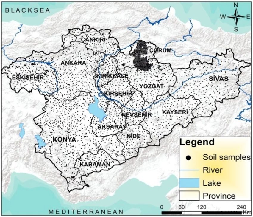
www.nature.com/scientificreports/
Figure 3. Soil samples in the study area (the map was created by the authors using the ArcGIS 10.2, http://esri.
com).
account the indicator eligibility of representing one or more of the soil characteristics, nine different evaluation
parameters, which are affecting plant growth in agricultural suitability index and also proposed/used by De La
Rosa et al. (1981)40, Dengiz (2007)41, Hazelton and Murphy (2007)42, Iojă et al. (2014)43, Zhang et al. (2015)29,
Mustafa et al. (2017)44, Demirağ Turan and Dengiz (2017)45, Aldababseh et al. (2018)46, were selected. In this
current study, the following soil characteristic: soil texture, OM, BD, pH, and C aCO3 were suggested by many
researchers due to their effects on water holding capacity, pore size, soil structure, and aggregate stability, root
growth, soil fertility, availability plant nutrient elements, e tc47–49. Demirağ Turan et al. (2019)50 indicated that soil
organic matter content represents a key indicator for soil quality, both for agricultural functions (i.e. produc-
tion and economy) and for environmental functions (i.e. carbon sequestration and air quality). Lime content of
soil in cultivated area is main reason for available nutrient element behaviour and influences also soil reaction.
According to Eyüpoğlu (1999)51 lime (CaCO3) content of Turkey’s territory has been studied and it was deter-
mined that 58.6% of the territory is calcareous soils due to parent material and low precipitation and located
mostly around Central Anatolia Region. In addition, some land characteristics such as slope, depth, erosion,
parent material have also crucial role for arable lands. Particularly increasing of slope degree negatively influ-
ences the drainage-irrigation and field traffic or mechanization p ractices41,52. In addition, the high slope degree
causes along the risk of soil erosion and this leads to organic matter and nutrient loss, especially in surface soil53.
For these reasons, slope factor has been adopted and used as a limiting factor for land suitability in the arable
land according to the FAO F ramework54. Selected parameters and activities for identifying potential agricultural
areas are presented in Table 1.
Karaca et al. (2020)70 reported that it was generally accepted that land and soil quality indicators can be
separated as either inherent or dynamic. The inherent factors are for example soil texture or mineralogical
composition, while the dynamic characteristic pointed out that dynamic factors are considered to evaluate how
soil management decisions affect soil properties. This study was performed at reginal scale. That is why, mostly
the inherent indictors were preferred for site suitability of potential agricultural land. A total of nine criteria
were used, as four terrain properties including slope, depth, erosion, and parent material and five soil features
including organic matter, bulk density (BD), texture, pH and lime content (CaCO3), in this study to identify
potential sites suitable for agriculture uses. Also, classifications for each criterion have been created and scores
between 1 and 4 are given for classifications each of these classifications to identify the suitability for potential
agricultural activities. If criteria classifications are at an optimum level of suitability for potential agriculture
uses, they are scored as 1 and if they have low suitability, they are scored as 4. Between two values is evaluated
as classifying factor and degree (Table 2).
The relative importance of these criteria should be determined (weighting) since they are not equally effec-
tive in identifying potential agriculture areas. In this study, the FAHP method was used to weight the criteria.
Detailed information about the method is included in the following sections of the study.
Once the relative importance levels of the criteria have been determined, the Weighted Linear Combination
(WLC) method was used for the identification of potential agricultural areas. WLC is also known as simple
additive weighting (SAW), weighted calculation, weighted linear mean and weighted thrust71. WLC method
calculates the value of the suitability of a potential region by using the formula in Eq. (2).
Scientific Reports | (2020) 10:22074 | https://doi.org/10.1038/s41598-020-79105-4 5
Vol.:(0123456789)www.nature.com/scientificreports/
Criterion Effectiveness Literatures
Sarkar et al., 201455; Bandyopadhyay
Depth Root development, water retention
et al. (2009)56
FAO, 197657; Feizizadeh and
Slope Field traffic, runoff,
Blaschke, 201258
Land criteria
Dengiz, 200741; Demirağ Turan and Dengiz,
Erosion Soil loss
201745
Bera et al., 201759; Pramanik, 201660; Dengiz et al.,
Parent material Soil formation
201961
Infiltration, structure development, soil–water
Texture Ahmed et al., 20164; Ashraf et al., 200262
relationship
Bulk density Soil compaction, aeration, infiltration Şeker ve Işıldar, 200063; Pagliai et al., 200364
Availability of nutrient elements, pH regulation in Gezgin and Hamurcu 200665; Feizizadeh and
Lime content
acid condition Blaschke, 201258
Soil criteria
Baridón et al., 201466; Feizizadeh and
pH Availability of nutrient elements, microbial activity
Blaschke, 201258
Riley et al., 200867; Kurzatkowski, 200468; Ban-
Organic Material Soil quality, biological activity dyopadhyay
et al., 2 00956; Guo et al., 201569
Table 1. Selected criteria for land suitability for agricultural usage and their effectiveness.
Land criteria
C2. Erosion (ton/
C. Parent material ha/year) C3. Soil depth (cm) C4. Slope (%)
Class Value Class Value Class Value Class Value
Alluvial deposits 1 0–5 1 0–20 4 0–2 1
Basic-ultrabasic magmatic and eruptions, melange, ophiolitic and
serpentine, shale, metamorphic rocks such as schist, phyllite clay 2 5–10 2 20–50 3 2–6 2
stone, marl
Siltstone, mudstone, conglomerate, travertine, limestone, dolo-
3 10–20 3 50–90 2 6–12 3
mite, marble
Acid magmatic, cherty, gneiss, dunes, volcanic ashes, tuff, agglom-
4 > 20 4 > 90 1 > 12 4
erate, breccia, evaporates, pebble stone, sand stone
Soil criteria
C6. Bulk density
C5. Organic matter (%) (g/cm3) C7. Texture C8. pH C9. CaCO3 (%)
Class Value Class Value Class Value Class Value Class Value
>3 1 1.0–1.2 1 Medium (L, Si, SiL, fSL) 1 6.5–7.5 1 0–5 1
3–2 2 1.2–1.4 2 Fine (C < %45, CL, SiL, SCL) 2 5.5–6.5 2 5–10 2
2–1 3 1.4–1.55 3 Very fine (fC > %45, SiCL, SC) 3 7.5–8.2 3 10–20 3
0–1 4 > 1.55 4 Coarse (S, SL, LS) 4 < 5.5- > 8.2 4 > 20 4
Table 2. Criteria, sub-criteria and their index values used for land suitability classes of agriculture usages.
l
Si = wk aik (2)
k=1
where (Eq. 2), Si represents the suitability value of the potential agricultural area; wk represents the relative
importance of the criterion k, aik represents the standard value under criterion k in i suitability area and l rep-
resents the total number of c riteria72.
After studies carried out considering the frequency distribution of values and statistical information, it is
considered appropriate to be shown in 5 classifications with Natural Breaks Jenks method73. This method is used
when data is not evenly distributed, there are huge differences between values and differences between classifica-
tions that need to be presented explicitly. Suitability classifications and index values for
these classifications for
potential agricultural areas are shown in Table 3.
Fuzzy logic sets. Zadeh (1965)74 first introduced the fuzzy set theory, whose application enables decision
makers to effectively deal with the uncertainties. In classical set theory, an element either belongs or does not
belong to the set. Fuzzy sets are sets whose elements have degrees of membership. A triangular fuzzy number
(TFN) is a type of fuzzy number and, according to Van Laarhoven and Pedrycz (1983)75, should possess the some
basic properties. The membership function of the TFN is as f ollows76:
Scientific Reports | (2020) 10:22074 | https://doi.org/10.1038/s41598-020-79105-4 6
Vol:.(1234567890)www.nature.com/scientificreports/
Class Index Definition
S1 1.33–1.91 Very high suitable
S2 1.92–2.24 High suitable
S3 2.25–2.52 Marginally suitable
N1 2.53–2,79 Currently non suitable
N2 2.80–3.95 Permanently non suitable
Table 3. Land suitability classes and their index values for agriculture usages.
∼ ∼
A fuzzy number A on R to be TFN if it is membership function x ∈A, µ∼ (x) : R → [0, 1] is equal to
A
(x − l)/(m − l), l ≤ x ≤ m,
µ∼ (x) = (u − x)/(u − m), m ≤ x ≤ u, (3)
A
0, otherwise
∼
where l and u stand fort he lower and upper ∼ bounds of the fuzzy number A , respectively, and m for the
modal
∼ value. The TFN∼ can be denoted by A= (l, m, u) and the following is the operational laws of two TFNs
A1 = (l1 , m1 , u1 ) and A2 = (l2 , m2 , u2 ).
Addition of fuzzy number ⊕
∼ ∼
A1 ⊕ A2 = (l1 + l2 , m1 + m2 , u1 + u2 ) (4)
Multiplication of a fuzzy number ⊗
∼ ∼
A1 ⊗ A2 = (l1 l2 , m1 m2 , u1 u2 ), (5)
for l1 l2 > 0; m1 m2 > 0; u1 u2 > 0
Subtraction of a fuzzy number ⊖
∼ ∼
A1 ⊖ A2 = (l1 − u2 , m1 − m2 , u1 − l2 ), (6)
Division of a fuzzy number ⊘
∼ ∼
A1 ⊘ A2 = (l1 /u2 , m1 /m2 , u1 /l2 ), (7)
for l1 l2 > 0; m1 m2 > 0; u1 u2 > 0
Reciprocal of a fuzzy number
∼ −1
A1 = (l1 , m1 , u1 )−1 = (1/u1 , 1/m1 , 1/l1 ) (8)
for l1 l2 > 0; m1 m2 > 0; u1 u2 > 0
Fuzzy‑AHP. The AHP method developed by Thomas L. Saaty is a mathematical method considering the
priorities of the group or individual, and evaluating qualitative and quantitative variables together in decision
making13. The AHP method is frequently used in solving multiple criteria decision-making problems since it is
easy to understand and includes simple mathematical calculations. However, the use of linguistic expressions
such as "very good", "good", "bad", and "very bad" instead of using numbers while decision-makers making pair-
wise comparisons during the implementation of the AHP method, is easier and better reflects the thinking style.
FAHP is introduced by integrating the traditional method with fuzzy logic in order to prevent this deficiency of
AHP method in decision making.
There are different FAHP methods proposed by different researchers in the literature18,75,77–79. Buckley (1985)18
calculates the fuzzy weights of the criteria using the geometric mean method. In this present study, Buckley’s
method was used to calculate criterion weights. The steps of the method implemented using Buckley’s method
are as follows.
Stage 1. Pairwise comparison matrices are created between all criteria in the hierarchical structure. Linguis-
tic expressions corresponding to pairwise ∼ comparison matrices are assigned by asking which is more important
for each of the two criteria as in matrix A.
∼ ∼ ∼ ∼
1 a 12 · · · a 1n 1 a 12 · · · a 1n
∼ ∼ ∼ ∼
∼ a 21 1 · · · a 2n 1/ a 21 1 · · · a 2n
=
A .
.. . .
=
. .
.. . . .
(9)
.. . . .. .. . . ..
∼ ∼ ∼ ∼
a n1 a n2 ··· 1 1/ a n1 a n2 · · · 1
where;
Scientific Reports | (2020) 10:22074 | https://doi.org/10.1038/s41598-020-79105-4 7
Vol.:(0123456789)www.nature.com/scientificreports/
Fuzzy number Linguistic scales Scale of triangular fuzzy number Scale of triangular reciprocal fuzzy number
∼
1 Equal (1,1,1) (1,1,1)
∼
2 Weak advantage (1,2,3) (1/3,1/2,1)
∼
3 Not bad (2,3,4) (1/4,1/3,1/2)
∼
4 Preferable (3,4,5) (1/5,1/4,1/3)
∼
5 Good (4,5,6) (1/6,1/5,1/4)
∼
6 Fairly good (5,6,7) (1/7,1/6,1/5)
∼
7 Very good (6,7,8) (1/8,1/7,1/6)
∼
8 Absolute (7,8,9) (1/9,1/8,1/7)
∼
9 Perfect (8,9,10) (1/10,1/9,1/8)
Table 4. Triangular fuzzy conversion scale.
1̃, 2̃, 3̃, 4̃, 5̃, 6̃, 7̃, 8̃, 9̃
aij = 1
−1 −1 −1 −1 −1 −1 −1 −1 −1
1̃ , 2̃ , 3̃ , 4̃ , 5̃ , 6̃ , 7̃ , 8̃ , 9̃
criterion i is relative importance to criterion j
i=j
criterion i is relative less importance to criterion j
Stage 2. Linguistic expressions in pairwise comparison matrices are converted to triangular fuzzy numbers.
In this study, the scale created by Gumus (2009)80 was used for the conversion of linguistic expressions into
triangular fuzzy numbers (Table 4).
Stage 3. The geometric mean technique proposed by Buckley (1985)18 is used to calculate the fuzzy geomet-
ric mean and fuzzy weight of each criterion.
∼
∼ ∼ ∼
1/n
r i = a i1 ⊗ a i2 ⊗ · · · ⊗ a in (10)
∼ ∼ ∼ −1
∼
wi = r i ⊗ r 1 ⊕ · · · ⊕ r n (11)
∼ ∼
a in is a fuzzy pairwise comparison value of criteria i. and criteria∼n. Accordingly, r i is the geometric mean of
the∼fuzzy pairwise comparison value of criteria i. with each criterion. w i is fuzzy weight of criteria i . and expressed
as w i = (lw i , mw i , uw i ). lw i, mw i and uw i represents the lower, middle and upper values of fuzzy weight of criteria
i, respectively.
Stage 4. The criterion weights obtained are a triangular fuzzy number. Fuzzy numbers should be clarified to
be converted into real numbers. The Center of Area (COA) method is one of the commonly used clarification
methods because it is∼ a simple and practical method81. The Best Non-fuzzy Performance (BNP) value of trian-
gular fuzzy number w i is calculated by the formula in Eq. (12).
(uw i − lw i ) + (mw i − lw i )
BNP i = lw i + , ∀i. (12)
3
Results and discussion
Some soil physico‑chemical properties. The some physical and chemical properties considered in this
study showed variability as a result of dynamic interactions among natural environmental factors, including the
degree of soil development and land use land cover types. Descriptive statistics of soil properties were given in
Table 5. The value of pH in soil samples ranged between 6.40 and 9.47, BD had maximum 1.84, minimum 0.72
gr/cm3. In addition, minimum and maximum values of C aCO3 varied from 0.01% to 95.24% while, OM varied
between 0.42% and 13.0%. Moreover, clay varied between 0.42% and 80.94%, silt varied between 1.01% and
81.16%, sandy varied between 1.38% and 93.84%. The texture components of basin soils exhibit normal distribu-
tions of clay, silt and sand content. On the other hand, other properties don’t exhibit normal distribution. The pH
and BD show skewness characteristics to the left and OM, C aCO3, clay, silt and sand content have skewness char-
acteristics to the right. The CV is the most important factor in defining the variability of soil properties82. If the
Scientific Reports | (2020) 10:22074 | https://doi.org/10.1038/s41598-020-79105-4 8
Vol:.(1234567890)www.nature.com/scientificreports/
Criteria Mean SD CV Variance Min Max Skewness Kurtosis
Clay (%) 29.03 13.43 80.51 190.45 0.43 80.94 0.36 − 0.22
Silt (%) 25.90 9.43 80.14 89.07 1.01 81.16 0.47 1.55
Sand (%) 43.98 16.68 92.46 278.51 1.38 93.84 0.24 − 0.26
BD (g/cm3) 1.37 0.13 1.11 0.02 0.72 1.84 -0.08 − 0.31
pH 7.60 0.48 5.03 0.23 6.40 9.47 -0.91 3.27
CaCO3 (%) 16.72 15.36 95.23 236.23 0.01 95.24 1.21 1.32
OM (%) 1.70 1.23 13.0 1.65 0.86 13.0 2.15 8.89
Table 5. Descriptive statistics some physico-chemical properties of soil samples. OM organic matter, BD bulk
density, SD standard deviation, CV coefficient of variation, Min minimum, Max maximum.
Soil criteria
Interpolation models Semivariogram modeller OM BD pH CaCO3 Texture
IDW-1 1.139 0.128 3.245 11.963 12.099
Inverse distance weighting (IDW) IDW-2 1.197 0.133 3.559 12.226 12.465
IDW-3 1.269 0.138 3.841 12.655 12.985
TPS 6.285 1.955 4.837 11.798 12.098
Radial basis functions (RBF) CRS 1.157 0.125 3.187 11.745 12.012
SWT 1.172 0.125 3.183 11.787 12.013
Gaussian 1.148 0.127 3.096 12.155 12.256
Ordinary Exponential 1.145 0.128 3.147 11.875 12.158
Spherical 1.149 0.127 3.114 11.988 12.198
Gaussian 1.132 0.363 3.136 12.231 19.897
Kriging Simple Exponential 1.135 0.135 3.793 11.910 12.688
Spherical 1.123 0.139 3.222 12.094 13.280
Gaussian 1.148 0.126 3.096 12.155 12.256
Universal Exponential 1.145 0.128 3.147 11.875 12.158
Spherical 1.149 0.127 3.114 11.988 12.198
Table 6. Interpolation models and RMSE of soil criteria. TPS thin plate spline, CRS completely regularized
spline, SWT spline with tension, OM organic matter, BD bulk density.
CV value is ≤ 15%, between 15 and 30%, or ≥ 30%, the variability is low, medium or high83. In this study, the low-
est and highest CVs obtained for soil samples were 1.11% for BD, and 95.23% for CaCO3 content, respectively.
Determination of the suitable interpolation model. Fifteen interpolation models were applied in
order to create soil criteria distribution maps and the lowest RMSE values found are given in Table 6. Accord-
ing to this, Kriging Simple Spherical model was determined as the most suitable for organic substance, Radial
Basis Functions Spline with Tension was determined as the most suitable for volume weight, and Kriging Simple
Gaussian model was determined as the most suitable for pH. Also, Radial Basis Functions Completely Regular-
ized Spline was determined as the most suitable for lime and texture in order to generate their spatial distribu-
tion maps.
Determination of the criteria weight with FAHP. A decision-making team consisting of three experts
was formed at application stage. Nine criteria were determined to be used in the study of identifying the areas
suitable for potential agriculture in the study area with the literature support and the opinions of the expert team,
and these criteria can be found in Table 2. These criteria representing the land and soil characteristics of the
region have different importance levels in determining the areas suitable for agriculture. In this study, the FAHP
method was used to weight the criteria.
Firstly, decision-makers were asked to make pairwise comparisons using the linguistic scale in Table 4 in
determining the criterion weights. Values obtained in the pairwise comparison process are determined as a
result of the joint study of decision-making team members. The fuzzy numbers corresponding to the linguistic
expressions obtained as a result of pairwise comparisons are given in Table 7. Pairwise comparison values were
converted to triangular fuzzy numbers using the scale in Table 8. ∼
After the pairwise comparison matrix was transformed into triangular ∼
fuzzy numbers, firstly r i value was
calculated by using Eq. (10) to calculate the fuzzy weights of criteria. For 1 as example:
r
Scientific Reports | (2020) 10:22074 | https://doi.org/10.1038/s41598-020-79105-4 9
Vol.:(0123456789)www.nature.com/scientificreports/
C.1 C.2 C.3 C.4 C.5 C.6 C.7 C.8 C.9
∼−1 ∼−1 ∼−1 ∼−1 ∼−1 ∼−1 ∼−1 ∼
C.1 1 3 3 5 5 2 3 2 2
∼ ∼−1 ∼−1 ∼ ∼ ∼ ∼ ∼
C.2 3 1 3 3 3 3 3 5 5
∼ ∼ ∼−1 ∼ ∼ ∼ ∼ ∼
C.3 3 3 1 1 3 5 3 3 5
∼ ∼ ∼ ∼ ∼ ∼ ∼
C.4 5 3 1 1 5 5 2 5 5
∼ ∼−1 ∼−1 ∼−1 ∼ ∼−1 ∼ ∼
C.5 5 3 3 5 1 3 3 3 5
∼ ∼−1 ∼−1 ∼−1 ∼−1 ∼−1 ∼ ∼
C.6 2 3 5 5 3 1 3 3 5
∼ ∼−1 ∼−1 ∼−1 ∼ ∼ ∼ ∼
C.7 3 3 3 2 3 3 1 2 5
∼ ∼−1 ∼−1 ∼−1 ∼−1 ∼−1 ∼−1 ∼
C.8 2 5 3 5 3 3 2 1 3
∼−1 ∼−1 ∼−1 ∼−1 ∼−1 ∼−1 ∼−1 ∼−1
C.9 2 5 5 5 5 5 5 3 1
Table 7. Pairwise comparison matrix.
C.1 C.2 C.3 C.4 C.5 C.6 C.7 C.8 C.9
C.1 (1, 1, 1) (1/4, 1/3, 1/2) (1/4, 1/3, 1/2) (1/6, 1/5, 1/4) (1/6, 1/5, 1/4) (1/3, 1/2, 1) (1/4, 1/3, 1/2) (1/3, 1/2, 1) (1, 2, 3)
C.2 (2, 3, 4) (1, 1, 1) (1/4, 1/3, 1/2) (1/4, 1/3, 1/2) (2, 3, 4) (2, 3, 4) (2, 3, 4) (4, 5, 6) (4, 5, 6)
C.3 (2, 3, 4) (2, 3, 4) (1, 1, 1) (1, 1, 1) (2, 3, 4) (4, 5, 6) (2, 3, 4) (2, 3, 4) (4, 5, 6)
C.4 (4, 5, 6) (2, 3, 4) (1, 1, 1) (1, 1, 1) (2, 3, 4) (4, 5, 6) (1, 2, 3) (4, 5, 6) (4, 5, 6)
C.5 (4, 5, 6) (1/4, 1/3, 1/2) (1/4, 1/3, 1/2) (1/6, 1/5, 1/4) (1, 1, 1) (2, 3, 4) (1/4, 1/3, 1/2) (2, 3, 4) (4, 5, 6)
C.6 (1, 2, 3) (1/4, 1/3, 1/2) (1/6, 1/5, 1/4) (1/6, 1/5, 1/4) (1/4, 1/3, 1/2) (1, 1, 1) (1/4, 1/3, 1/2) (2, 3, 4) (4, 5, 6)
C.7 (2, 3, 4) (1/4, 1/3, 1/2) (1/4, 1/3, 1/2) (1/3, 1/2, 1) (2, 3, 4) (2, 3, 4) (1, 1, 1) (1, 2, 3) (4, 5, 6)
C.8 (1, 2, 3) (1/6, 1/5, 1/4) (1/4, 1/3, 1/2) (1/6, 1/5, 1/4) (1/4, 1/3, 1/2) (1/4, 1/3, 1/2) (1/3, 1/2, 1) (1, 1, 1) (2, 3, 4)
C.9 (1/3, 1/2, 1) (1/6, 1/5, 1/4) (1/6, 1/5, 1/4) (1/6, 1/5, 1/4) (1/6, 1/5, 1/4) (1/6, 1/5, 1/4) (1/6, 1/5, 1/4) (1/4, 1/3, 1/2) (1,1,1)
Table 8. Fuzzy pairwise comparison matrix.
∼
1/9
= 1 × ( 41 × 41 × 16 × 61 × 13 × 41 × 13 ) × 1 , (1 × ( 13 ) × ( 13 ) × ( 15 ) × ( 15 ) × ( 21 ) × ( 13 )
r1
1/9
×( 21 ) × 2) ,
1/9
(1 × ( 12 ) × ( 12 ) × ( 41 ) × ( 41 ) × 1 × ( 21 ) × 1 × 3) = (0.331, 0.449, 0.659)
∼
Similarly, the remaining r i values were calculated, there are:
∼ ∼ ∼ ∼ ∼
r 2 =(1.361,1.825,2.364), r 3 =(2.000,2.633,3.217), r 4 =(2.333,2.984,3.566), r 5 =(0.819,1.058,1.379), r 6 =
∼ ∼ ∼
(0.533,0.708,0.938),
∼
r 7 =(0.956,1.351,1.876), r 8 =(0.404,0.548,0.769),
∼
r 9 =(0.230,0.280,0.367)
Then,
∼
w i values were calculated using Eq. (11). For w 1 as example:
w 1 = (0.331, 0.449, 0.659)⊗ (1/(0.659 + 2.364 + 3.217 + 3.566 + 1.379 + 0.938 + 1.876 + 0.769 + 0.367),
1/(0.449 + 1.825 + 2.633 + 2.984 + 1.058 + 0.708 + 1.351 + 0.548 + 0.280), 1/(0.331+1.361
+2.000 + 2.333 + 0.819 + 0.533
∼
+ 0.956 + 0.404 + 0.230)) = (0.022, 0.038, 0.073)
Similarly,
∼
the remaining w∼i values were calculated, there
∼
are: ∼ ∼
w 2 =(0.090,0.154,0.264), w 3 =(0.132,0.222,0.359), w 4 =(0.154,0.252,0.398), w 5 =(0.054,0.089,0.154),w 6 =
∼ ∼ ∼
(0.035,0.060,0.105),w 7 =(0.063,0.114,0.209), w 8 =(0.027,0.046,0.086),w 9 =(0.015,0.024,0.041)
The COA defuzzification method (Eq. 12) was used to calculate BNP weights of criteria. For BNP 1 as example:
BNP 1 = 0.022 + [(0.073 − 0.022) + (0.038 − 0.022)]/3 = 0.044
Similarly, the remaining BNP weights of criteria were calculated. After all BNP scores are calculated, nor-
malization is performed for all BNP values.
In regional studies, although the weight value, such as the parent material and lime content, which have lit-
tle effect on potential agricultural suitability, is lower than other parameters, the degree of slope and effective
soil depth which are factors that improving or replacing in the land is the limiting factor for non-economic and
agricultural mechanization activities were determined as the criteria with highest weight values. Also, the higher
weighting is recommended for properties that pose a continuous risk (erosion)4,11,84. Besides, it is known that
parameters, which the presence in the environment is not absolutely necessary for vegetative production however
effective on soil quality (e.g. organic matter), should have a moderate weight r atio67. Based on these evaluations,
which the weight values obtained considering the region ecology, the degree of influence of the criteria for
Scientific Reports | (2020) 10:22074 | https://doi.org/10.1038/s41598-020-79105-4 10
Vol:.(1234567890)www.nature.com/scientificreports/
determining potential agricultural land was evaluated in 3 groups as high, moderate and low. It was determined
that slope (0.245), depth (0.217) and erosion (0.155) criteria are high and texture (0.118), organic matter (0.091)
and bulk density (0.061) moderate weight and pH (0.48), parent material (0.041) and lime content (0.024) are
low coefficients. As can be seen in this order, the slope criterion with a weight value of 0.245, has obtained as
the criterion with the highest weight. Dengiz and Sarıoğlu (2013)11 found similar results in their studies and
proposed slope should not exceed 10–12% for cultivation without taking soil erosion measures or taking very
few measures and therefore, Verdoodt and Van Ranst (2003)85 stated that slope is the most important criterion
in land capability classification and agriculture practices in field. Because, slope plays an important role in soil
erosion and has performing the activities correctly such as in-field mechanization or field traffic. Depth and ero-
sion come in second and third place among the high classification for the criteria being addressed. These criteria
are closely related to the retention of water and plant nutrients in the soil and land capability classification, soil
fertility and quality characteristics such as plant root development 41,86. Considering the ecological characteristics
of the region, the parent material in terms of its contribution to soil formation and some agricultural applications
(pH regulators, fertilization, etc.) for eliminating the adverse effects of CaCO3 content and soil reaction, led the
weight values of these criteria were determined to be low.
At the same time, the fact physical properties that can be improved by the improvement of land conditions
and organic matter enhancing applications are able to change land suitability and land quality classification
positively is an important factor in weighting. As a matter of fact, it is specified that mechanization is facilitated
and germination, plant output and yield values increased by the development of the structure by increasing
organic matter in agricultural land87,88. Besides, the positive effects of the organic matter on water retention,
soil compaction, aeration, and biological activity reduce the limiting effect of bulk density and available water
capacity and increase soil q uality68,69.
Spatial distribution of criteria and potential land suitability for agricultural usages. Site suit-
ability assessment for agricultural applications includes the assessment of a large amount and variety of internal
soil condition (depth, organic matter, texture, soil reaction etc.), and external soil conditions (topography, ero-
sion etc.).
The areal and proportional distributions of land and soil criteria for identifying the Central Anatolia potential
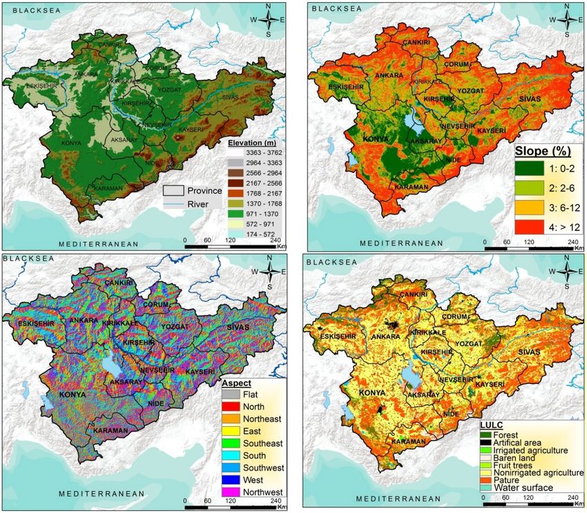
agricultural areas are given in Table 9 and Fig. 4. RUSLE (Revised Universal Soil Loss Equation) model was used
to estimate the spatial amount of erosion. It is observed that approximately 7% of Central Anatolia has severe and
very severe erosion risk whereas, 83.6% of the region has a slight or low risk of erosion. This situation is parallel
with the erosion severity classes of Turkey and according to Turkey’s water erosion a tlas89, the erosion risk of
country’s surface area consists of 60.28% very low, 19.13% lowt, 7.93% moderate, 5.97% severe and 6.7% very
severe. Kosmos et al. (2014)90 also used actual soil erosion to define categories of land quality risk, based on the
type of environmental sensitivity area (ESA) as an indicator for their empirical approach which was applied in 17
study areas in the Mediterranean region, Eastern Europe, Latin America, Africa and Asia. Moreover, Symeonakis
et al. (2014)91 estimated the ESAs on the island of Lesvos, Greece through a modified ESA, which included 10
additional indicators related to soil erosion, groundwater quality, demographics and grazing pressure between
two years, 1990 and 2000. Results showed that about 85% of the island is fragile or critically sensitive in both
periods: 81% in 1990 and 77% in 2000.
33.1% of the study area is considered deep, while 38.8% considered very deep for soil depth criterion, which is
an important parameter both in plant nutrient and water storage and root development in processed agricultural
applications10,46. Deep soils are mostly distributed in Konya, Aksaray, in some parts of Ankara, Çorum and Sivas,
which are located in the center of Central Anatolia, while shallow soils are widely distributed in the mountain-
ous areas around as well as Karaman, Çankırı, Yozgat and Kayseri provinces. Approximately half of the parent
material distribution of the study area (45.3%) consists of acid magmatic, cherty, gneiss, dunes, volcanic ashes,
tuff, agglomerate, breccia, evaporites, sand stone, while approximately one third (37.3%) consists of basic-ultra
basic magmatic and eruptions, melange, ophiolitic and serpentine, shale, etc. schist, metamorphic rocks, such
as phyllite, claystone, and marl. Only very little of the main material (0.3%) consists of young alluvial deposits.
The slope is considered as an important criterion in almost all of the areas for agricultural suitability in evalu-
ation studies. Therefore, the slope degree could be considered a restriction to land capability particularly for
irrigated agriculture Sauer et al. (2010)88 as it negatively restricts management and machinery applications such
as irrigation, tillage and drainage92 and determines the type of the irrigation system to be used and the flow rate,
hence affecting crop yields and irrigation cost. Slope also affects land productivity as high steep lands suffer from
soil loss41. According to Table 5, 64.3% of the Central Anatolian lands have a slope less than 12% slope which
is the limit value for machinery agriculture, while 35.7% has a high slope. The areas where the slope is flat and
moderately sloped are mostly distributed in the central area (Fig. 4). Most of the soils in the area (about 84%)
have very low organic matter content, which is usually between 1 and 2%. This situation is also in parallel with
Turkey Soil Organic Carbon Study93, the area has the highest 67.83 t C ha−1 soil organic carbon in the Black Sea
Region whereas, it has the second-lowest soil organic carbon stock with 38.5 t C ha-1 after Southeast Anatolia
Region (29.46 t C h a−1) due to low rainfall and vegetation effect.
Approximately 98% of the texture of the Central Anatolian soils are consisting of loam, clay loam, sandy clay
loam and clay (< 45% clay content), which are considered medium and fine classes, very few (3.0%) have very
fine (> 45% clay content) and coarse (sand, sandy loam and loamy sand) texture. In addition, more than 95% of
the soil has medium and high bulk density and they range from 1.21 gr c m−3 to 1.55 gr c m−3. Central Anatolia
Region lands do not contain soils with strong acid pH while more than half of the lands range from slightly to
moderate alkali. 16% of the soil has low lime content, while more than half of the lands have high and very high
content of lime.
Scientific Reports | (2020) 10:22074 | https://doi.org/10.1038/s41598-020-79105-4 11
Vol.:(0123456789)www.nature.com/scientificreports/
Area
Criteria Class Description ha %
1: 0–5 Very low 16,305,597 83.6
2: 5–10 Moderate 1,577,389 8.1
Erosion (ton/ha/year)
3: 10–20 High 924,183 4.7
4: 20 + Very high 694,102 3.6
1: 90 + Deep 3,818,409 19.6
Depth 2: 50–90 Moderate deep 2,637,154 13.5
(cm) 3: 20–50 Shallow 5,474,580 28.1
4: 0–20 Very shallow 7,571,129 38.8
1: 0–2 Flat 3,845,512 19.7
2: 2–6 Gently slope 4,360,510 22.4
Slope (%)
3: 6–12 Moderate slope 4,325,500 22.2
4: 12–20 High slope 6,969,750 35.7
1: – 59,250 0.3
2: – 7,267,910 37.3
Parent material
3: – 3,343,580 17.1
4: – 8,830,532 45.3
1: > 3 High 95,738 0.5
2: 3–2 Moderate 3,039,547 15.6
Organic matter (%)
3: 2–1 Low 11,840,528 60.7
4: < 1 Very low 4,525,459 23.2
1: 1.00–1.20 Low 806,082 4.1
2: 1.21–1.40 Moderate 10,760,485 55.2
Bulk density (g cm−3)
3: 1.41–1.55 High 7,832,192 40.2
4: > 1.55 Very high 102,513 0.5
1: Medium 10,300,571 52.8
2: Fine 8,607,234 44.1
Texture (%)
3: Very fine 182,112 0.9
4: Coarse 411,355 2.1
1: 6.5–7.5 Slightly acid or alkaline 8,997,319 46.1
2: 5.5–6.5 Slightly to moderate acid 178,496 0.9
pH
3: 7.5–8.5 Slightly to moderate alkaline 10,325,457 52.9
4: < 5.5- > 8.5 Strong acid or alkaline – –
1: 0–5 Low 3,121,923 16.0
2: 5–10 Moderate 5,849,441 30.0
Lime content-CaCO3 (%)
3: 10–20 High 9,401,612 48.2
4: > 20 Very high 1,128,296 5.8
Table 9. Spatial and proportional distribution of some criteria for land suitability for agriculture usages in
Central Anatolia Region.
As a result of the identification of potential agricultural lands of the study area by the FAHP approach, the
spatial and proportional distribution of the suitability classifications for each province is given in Table 10 and
Fig. 5. Approximately 30.7% (59,922 k m2) of the total area is determined as being very suitable and suitable for
agriculture uses at S1 and S2 levels, whereas 12.6% is not suitable for low-till agricultural activities. Potentially
suitable and very suitable areas for agriculture activities are mainly distributed among Konya, Aksaray, Nevşehir,
Kayseri, Yozgat, Kırşehir provinces. Areas of the region that are currently or not at all suitable (N1 and N2) for
agriculture uses are widely distributed in Sivas, Niğde, Çorum and Kırıkkale provinces and some areas are also
identified disconnectedly in the southern part of the study area. The most important factors that restrict agri-
cultural practices in these areas are high slope degree and shallow soil depth. Besides, it was determined that
26.6% of the area is slightly suitable (S3). Among the provinces, Konya has the largest surface area in the Central
Anatolia region with an area of 38,869.7 k m2, which corresponds to 19.9% of the total area and 2,354,450 ha
area of this area is very suitable (S1) and suitable (S2) areas for agricultural applications as the widest area in
the region, and Sivas province has the highest N1 and N2 suitability classes with an area of 19,571.6 k m2 in the
Central Anatolia region.
The land capability classification (LCC) system is put into classes ranging from best (Class I) to worst (Class
VIII) and gives an indication of the inherent capability of the land for general agricultural p roduction94. While it
can be assessed I, II, III classes of LCC system suitable for agricultural usage, IV class can be considered as slightly
Scientific Reports | (2020) 10:22074 | https://doi.org/10.1038/s41598-020-79105-4 12
Vol:.(1234567890)www.nature.com/scientificreports/
Figure 4. Spatial distribution of some criteria for land suitability for agriculture usages (the maps were created
by the authors using the ArcGIS 10.2, http://esri.com).
suitable for arable land and other classes are not suitable for cultivation area. General Directory of Rural S ervice95.
produced LCC maps in regional and national scales in Turkey. According to GDRS’s report, approximately 33.4%
of the total area was found as being in three classes for agriculture uses at I, II, and III, whereas 54.2% is not
suitable for agricultural applications. Moreover, it was determined that 12.4% of the area is slightly suitable (IV.
class). When compared to current results of the study, amount of agricultural suitable lands decreased about 2.7%,
whereas slightly suitable area was significantly changed from 12.4% to 26.6%. On the other hand in the current
study non-suitable area was determined 11.2% less. It can be said that these differences resulted from actuality
and quality of data, sensitive methodological approach and changings of land use managements.
Scientific Reports | (2020) 10:22074 | https://doi.org/10.1038/s41598-020-79105-4 13
Vol.:(0123456789)www.nature.com/scientificreports/
Suitability classes
Very high Marginally Currently non Permanently
suitable High suitable suitable suitable non suitable
Provinces S1 S2 S3 N1 N2
(km2) % km2 % km2 % km2 % km2 % km2 %
Aksaray (7905.1) 4.1 3041.5 1.6 2585.4 1.3 1912.5 1.0 365.8 0.2 0.0 0.0
Ankara (25,142.3) 12.9 1671.0 0.9 7044.5 3.6 7408.3 3.8 7631.0 3.9 1387.5 0.7
Bolu (1585.4) 0.8 119.5 0.1 246.3 0.1 502.8 0.3 554.4 0.3 162.5 0.1
Çankırı (8337.8) 4.3 0.0 0.0 360.0 0.2 2158.5 1.1 5051.0 2.6 768.3 0.4
Çorum (8346.8) 4.3 87.0 0.0 1587.3 0.8 3716.3 1.9 2773.8 1.4 182.5 0.1
Eskişehir (13,709.7) 7.0 1482.8 0.8 3482.8 1.8 3930.8 2.0 3858.2 2.0 955.3 0.5
Kırıkkale (4947.5) 2.6 0.0 0.0 613.5 0.3 1957.5 1.0 2202.5 1.1 174.0 0.1
Kırşehir (6750.7) 3.5 689.5 0.4 1011.5 0.5 3108.3 1.6 1677.0 0.9 264.5 0.1
Karabük (1120.3) 0.6 0.0 0.0 16.5 0.0 170.3 0.1 866.3 0.4 67.3 0.0
Karaman (8619.3) 4.4 1026.0 0.5 1150.8 0.6 983.8 0.5 2379.3 1.2 3079.5 1.6
Kayseri (17,030.2) 8.7 840.8 0.4 2153.8 1.1 4999.8 2.6 5305.3 2.7 3730.7 1.9
Konya (38,869.7) 19.9 11,201.7 5.7 12,342.8 6.3 5313.3 2.7 5947.5 3.0 4064.5 2.1
Nevşehir (5466.9) 2.8 52.3 0.0 1141.0 0.6 2764.5 1.4 1328.8 0.7 180.4 0.1
Niğde (6414.4) 3.3 762.3 0.4 1399.0 0.7 1313.5 0.7 1171.3 0.6 1768.2 0.9
Sivas (26,767.5) 13.9 56.3 0.0 893.8 0.5 6245.0 3.3 12,479.3 6.5 7092.6 3.7
Yozgat
7.2 15.0 0.0 2847.1 1.5 5360.1 2.6 5130.8 2.6 645.5 0.3
(13,999.3)
Total area (195,012.7) 100 21,045.7 10.8 38,876.1 19.9 51,845.3 26.6 58,722.3 30.1 24,523.3 12.6
Table 10. Land suitability classes for agriculture usages of each province in the Central Anatolia Region.
Conclusion
Identifying the suitability and quality of the lands has great importance for deciding on the use of land according
to its potential and protecting natural resources for future generations. In this study, identification of suitable
areas for agricultural land by taking soil and land indicators into account at regional scale carried out in the
Central Anatolia Region, which covers approximately 25% of Turkey with 78 million ha. In the current study,
land suitability for agriculture usages of the Central Anatolia Region was assessed on the basis of a comprehen-
sive set of criteria associated with multi criteria decision management taking into consideration of the FAHP
approach. The integration of fuzzy sets with AHP significantly contributed to the elimination of uncertainties
in expert opinions. In light of study results, it was seen that one third % of the study area has high and very
high suitable, whereas currently and permanently non suitable areas cover about half of the study area (42.7%),
suggesting that the areas are highly sensitive to agricultural activities or cultivations. However, when the results
are compared with CORINE 2012 land use-land cover, CORINE 2012 classification shows a distribution of
approximately 40% as agricultural area, while this study found that approximately 30% of the area is suitable for
agricultural activities but it is also found that agricultural activities take place in areas that are not suitable for
agriculture or in marginal agricultural areas, which corresponds approximately 12% of the area. Moreover, this
study can contribute important approach by applying fuzzy sets with AHP for land suitability for agriculture
usage estimation in regional scale.
Identification of suitable areas for agricultural fields is therefore based on the permanent biophysical features
of the land and does not take into account the economics of agricultural production, distance from markets,
social or political factors. That is why, this methodology should be integrated with thematic and/or detailed
additional information such as climate and socio-economic data, local land use processes and/or yield outputs,
and demographics to achieve more sensitive approach for determination of potential site suitability lands for
agriculture applications. Moreover, the results of the current study can guide the implementation of the strategic
objectives of the National Strategy and Action Plan in order to determine agricultural suitable area for sustain-
able land recourse.
Scientific Reports | (2020) 10:22074 | https://doi.org/10.1038/s41598-020-79105-4 14
Vol:.(1234567890)You can also read