If They Come, Where will We Build It? Land-Use Implications of Two Forest Conservation Policies in the Deep Creek Watershed - MDPI
←
→
Page content transcription
If your browser does not render page correctly, please read the page content below
Article
If They Come, Where will We Build It? Land-Use
Implications of Two Forest Conservation Policies in
the Deep Creek Watershed
Markandu Anputhas 1 , Johannus Janmaat 1, *, Craig Nichol 2 and Adam Wei 2
 1    Department of Economics, Philosophy and Political Science, I.K. Barber School of Arts and Sciences,
      The University of British Columbia, Kelowna, BC V1V 1V7, Canada
 2    Department of Earth, Environmental and Geographic Sciences, I.K. Barber School of Arts and Sciences,
      The University of British Columbia, Kelowna, BC V1V 1V7, Canada
 *    Correspondence: john.janmaat@ubc.ca; Tel.: +1-(250)-807-8021

 Received: 1 June 2019; Accepted: 9 July 2019; Published: 12 July 2019

 Abstract: Research Highlights: Forest conservation policies can drive land-use change to other
 land-use types. In multifunctional landscapes, forest conservation policies will therefore impact
 on other functions delivered by the landscape. Finding the best pattern of land use requires
 considering these interactions. Background and Objectives: Population growth continues to drive
 the development of land for urban purposes. Consequently, there is a loss of other land uses, such
 as agriculture and forested lands. Efforts to conserve one type of land use will drive more change
 onto other land uses. Absent effective collaboration among affected communities and relevant
 institutional agents, unexpected and undesirable land-use change may occur. Materials and Methods:
 A CLUE-S (Conversion of Land Use and its Effects at Small Scales) model was developed for the
 Deep Creek watershed, a small sub-basin in the Okanagan Valley of British Columbia, Canada.
 The valley is experiencing among the most rapid population growth of any region in Canada.
 Land uses were aggregated into one forested land-use type, one urban land-use type, and three
 agricultural types. Land-use change was simulated for combinations of two forest conservation
 policies. Changes are categorized by location, land type, and an existing agricultural land policy.
 Results: Forest conservation policies drive land conversion onto agricultural land and may increase
 the loss of low elevation forested land. Model results show where the greatest pressure for removing
 land from agriculture is likely to occur for each scenario. As an important corridor for species
 movement, the loss of low elevation forest land may have serious impacts on habitat connectivity.
 Conclusions: Forest conservation policies that do not account for feedbacks can have unintended
 consequences, such as increasing conversion pressures on other valued land uses. To avoid surprises,
 land-use planners and policy makers need to consider these interactions. Models such as CLUE-S can
 help identify these spatial impacts.

 Keywords: land-use change; land-use forecasting; agricultural land; forest land; forest conservation;
 land-use policy; unintended consequences; complex systems

1. Introduction
      In the 1989 movie “Field of Dreams [1],” the main character hears a mysterious voice say, “If you
build it, he will come.” This initiates a drama where the main character overcomes various challenges
to build a baseball diamond in the middle of a corn field, a diamond which attracts the spirits of many
deceased baseball heroes to play their beloved game. Most of the rest of the world is burdened with a
different challenge. They are coming, and we do not know where they will live. Hence, our challenge
is, “If they come, where will we build it?”

Forests 2019, 10, 581; doi:10.3390/f10070581                                      www.mdpi.com/journal/forests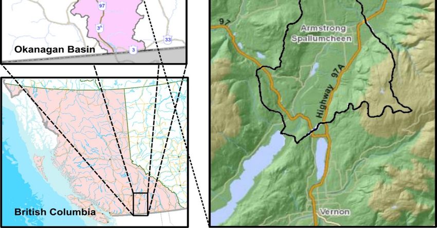
Forests 2019, 10, 581                                                                                2 of 20

      British Columbia is a largely mountainous province with extensive areas of forest, with the forest
industry contributing approximately three percent of provincial GDP [2]. British Columbia’s forests
also provide many non-timber services that residents’ value, including recreational opportunities,
wildlife habitat, carbon storage, and landscape aesthetics. These services are generally diminished
when forests are harvested, with civil society having a long history of public action in the province to
protect forested areas of high value [3,4]. In some cases, these high value forests have strong symbolic
appeal, while in other cases the high value forests are valued because they are close to communities
where people live. This latter value tends to create pressure for protection of public forested land near
urban areas. At the same time, the desire of people to live in the interface regions between urban areas
and forests has led to development pressure, evidenced by strong demand for housing in the interface
area, on privately held forested land.
      Agriculture is also an important industry in British Columbia, contributing approximately twice
as much to the provincial GDP as forestry [2]. Less than five percent of the provincial land base is
considered arable, with most of that located in valley bottoms along rivers and lakes [5]. These areas
are also attractive for human settlement, leading to substantial development pressures on this limited
agricultural land base [5,6]. There is a long history of public support for protecting agricultural land in
the province, witnessed by the passing of the Agricultural Land Commission Act in 1973, and continued
public support for the Agricultural Land Reserve (ALR) created by that Act [7]. The ALR is a provincial
level land-use zone that includes land of suitable agricultural potential, with uses within that zone in
principle limited to activities that do not impact on the ability of the land to be used for agriculture.
The ALR is a land reserve, with only about half of the land within the ALR actually being farmed [6].
Land that has been used for development purposes is generally excluded from the ALR, while land
that could be brought into production, such as currently forested land with high agricultural potential,
is often within the reserve. Exclusions of land currently within the reserve, generally done when
such land is developed for urban uses, must in most cases be approved by the Agricultural Land
Commission [8].
      The authority to direct land-use decisions in British Columbia is fragmented. Jurisdiction over
land within the ALR is largely the responsibility of the Agricultural Land Commission, which interacts
with the provincial Ministry of Agriculture (formerly BC Ministry of Agriculture and Lands, BCMAL).
This ministry is charged with enhancing the economic contribution of agriculture within the province [9].
Jurisdiction over forest and range crown lands lies in large part with the Ministry of Forests, Lands,
Natural Resource Operations and Rural Development. This ministry is responsible for the stewardship
of provincial Crown land and natural resources [10]. Regulation of the use of private land that is not
within the ALR is largely the responsibility of local governments, municipalities, and regional districts
that write and enforce zoning bylaws for their area of responsibility [11]. Local governments often
prioritize development, which with immigration creates jobs, increases property prices, and the local
tax base. Development is often the highest value land use, and as such land owners, who are often
well represented in local government, are typically looking for ways to develop their land and realize
this highest value.
      Policy choices by these different agencies are often made in isolation, and unintended consequences
can be the result. In this paper we use a land-use change model to examine how policies aimed at
protecting forests can have such unintended consequences on other land uses that society values. In
the next section we describe the watershed that is the subject of our land-use change model. We then
turn to describing the modeling system we chose to use, the CLUE-S system [12,13], with a brief
discussion of its implementation and validation. The results follow. Results are developed for four
different land-use policy scenarios. These results are described in relation to the ALR, and to their
impact on the location and pattern of land-use change in the watershed. Prior to a short conclusion,
results are discussed, examining their implications for policy and extensions of this analysis using
alternative land-use change forecasting methods.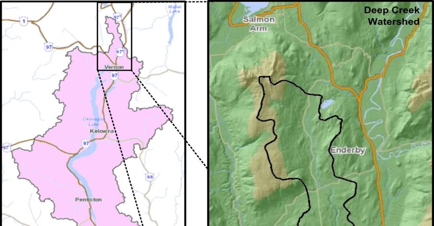
Forests 2019, 10, 581                                                                                               3 of 20

2. Materials and Methods
   Forests 2019, 10, x FOR PEER REVIEW                                                                           3 of 20

2.1. Study Site
   2.1. Study Site
      The Deep Creek watershed is located in the northern portion of the Okanagan Valley, in the
         The Deep Creek watershed is located in the northern portion of the Okanagan Valley,         in the
                                                                                                   2 with
southern part of British Columbia (Figure 1). The watershed covers an area of 230 km                        the
   southern part of British Columbia (Figure 1). The watershed covers an area of 230 km with the 2
elevation varies between 340 and 1580 m elevation above sea level [14]. Deep Creek falls under the
   elevation varies between 340 and 1580 m elevation above sea level [14]. Deep Creek falls under the
North Okanagan basin eco-section of Thompson–Okanagan Plateau eco-region [15]. At present, more
   North Okanagan basin eco-section of Thompson–Okanagan Plateau eco-region [15]. At present, more
than  half
   than    of the
         half      watershed
              of the watershedarea is undeveloped
                                 area is undeveloped forested  land.
                                                        forested land.Montane forest
                                                                        Montane      types
                                                                                forest     ofof
                                                                                       types  Douglas
                                                                                                Douglasfirfir
                                                                                                           and
Lodgepole     pine are
   and Lodgepole       extensively
                    pine            foundfound
                         are extensively   in theinwatershed   [15].[15].
                                                    the watershed

           Figure 1. 1.Location
             Figure     LocationofofDeep
                                     DeepCreek
                                         Creekwatershed
                                               watershed in Okanaganbasin
                                                         in Okanagan basinofofBritish
                                                                               BritishColumbia,
                                                                                       Columbia, Canada.
                                                                                                Canada.

      The
        Thevalley
             valleyhas
                     hasone
                         oneofofthe
                                  thehighest
                                      highestrates
                                               rates of
                                                      of population      growthin
                                                         population growth        inCanada
                                                                                     Canada[16,17].
                                                                                               [16,17].The
                                                                                                         The  population
                                                                                                           population
trends  for the City  of Armstrong,     Township     of  Spallumcheen       (Armstrong–Spallumcheen
   trends for the City of Armstrong, Township of Spallumcheen (Armstrong–Spallumcheen local health           local  health
area), thethe
   area),  Regional   District
               Regional        of Columbia–Shuswap
                          District   of Columbia–Shuswap    (RDCS),    and the
                                                                 (RDCS),        Regional
                                                                              and          DistrictDistrict
                                                                                    the Regional     of NorthofOkanagan
                                                                                                                 North
(RDNO)    show(RDNO)
   Okanagan      steady positive    growth
                          show steady        [18]. This
                                          positive        growth
                                                     growth    [18].is This
                                                                       not spatially
                                                                             growth isuniform.   The population
                                                                                         not spatially   uniform. Theof the
City  of Armstrong
   population   of the was
                       City 4850   in 2011 and
                            of Armstrong      wasthe
                                                   4850population
                                                          in 2011 and  change   from 2006
                                                                          the population     to 2011
                                                                                          change   fromwas  13.4%
                                                                                                          2006      while
                                                                                                               to 2011
thewas
     population   of the
        13.4% while   therural   Township
                          population    of theofrural
                                                 Spallumcheen
                                                      Township of    increased   from 4960
                                                                        Spallumcheen          to 5055
                                                                                        increased   fromduring  the5055
                                                                                                          4960 to    same
   during the same period, an increase of 1.9% [16,17]. The dry, relatively warm climate makes the
Forests 2019, 10, 581 4 of 20
period, an increase of 1.9% [16,17]. The dry, relatively warm climate makes the Okanagan Valley an
attractive destination for amenity migrants, with those migrants demanding housing and other goods
and services [19,20].
The northern portion of the watershed lies within the Regional District of Columbia-Shuswap
(RDCS), with the majority contained in the Regional District of North Okanagan (RDNO). Salmon Arm,
Armstrong, and Vernon are the major cities that can be easily accessed from within the watershed
(Figure 1). Highways 97A and 97B join Vernon and Salmon Arm via Armstrong. This highway travels
through the south east portion of the watershed, and then follows a route outside the watershed,
along its east and north. Road access in the northern part of the watershed connects to highway 97B.
Access to transportation and markets is important for many activities. Farmers need roads to access
markets for inputs and to deliver products for sale. Residents use roads to access employment and
retail. Much of the Deep Creek watershed is rural residential, with many jobs located in the cities of
Vernon and Salmon Arm, both just outside the watershed (Figure 1). Distance to urban centers and
access to transportation are important for livelihood activities of the residents in the watershed.
Forestry, agriculture, manufacturing, and tourism are all important economic activities in the
watershed. Agriculture is particularly significant in the valley bottom. Livestock farming is the most
common category of farming, representing about 21% of all agricultural operations in the Township
of Spallumcheen.
2.2. The CLUE-S Modeling System
We used the Conversion of Land Use and its Effects in Smaller scale (CLUE-S) [12,13,21] system,
which has proven to be an effective tool for modelling fairly fine scale land-use change. It has been
used as land-use change projection tool in African, Asian, American, and European locations [22–27].
This modeling exercise was part of a larger research effort aimed at projecting the impact of climate
change on the hydrology of the Deep Creek watershed, similar to [28]. Agriculture is a significant
water user within the watershed [14], with predicted changes in agricultural activities therefore being
an important part of forecasting impacts on the hydrology of the watershed. Surface and groundwater
processes were modeled using MIKE SHE [29], with climate change projections downscaled to a
500 m × 500 m grid resolution [30]. Given that MIKE SHE is a proprietary product with limited capacity
for coupling to a land-use model, it would not be possible to integrate feedbacks between changes in
climate and hydrology with land-use decisions. A process-based (e.g., agent-based) land-use change
model would therefore miss important drivers, making a pattern-based model both a practical and
appropriate approach. Among the set of possible pattern-based models, CLUE-S fit the data availability
and needs of the larger project.
A CLUE-S model evolves a gridded map of the study landscape forward, using a probabilistic
transition model to forecast land-use changes of individual grid cells. CLUE-S is parameterized using
an observation of the landscape at one point in time, with multiple variables measured for each grid
cell. Transition probabilities are estimated using a set of logistic regressions, with each land-use type
predicted as a function of a set of explanatory variables observed at each cell. The observed relationship
between land use and the explanatory variables is assumed to continue forward in time and to be
constant across the landscape. CLUE-S does not forecast how much land use will change but rather
where changes will take place. Changing trends in aggregate land-use types across the study are taken
from other sources. The land-use type of individual grid cells changes as the simulation progresses to
match the provided aggregate changes. For this exercise, the growth in urban area is expected to reflect
population growth projections [18]. Changes in the relative composition of agricultural activities is
taken to be a continuation of past trends [31,32]. “Forest and range” serves as a residual land-use
category, adjusted to account for projected changes in the other four land-use categories. See [33] for
details of our model construction.
Within CLUE-S, spatial restrictions can be imposed to reduce land-use change or protect a
particular land use in an area of the simulated landscape (see for examples [27,34,35]). We use thisForests 2019, 10, 581 5 of 20
Forests 2019, 10, x FOR PEER REVIEW
feature to examine the impacts of two different spatial land-use policies on the evolution of land5use
of 20
in
the Deep Creek watershed.
2.2.1. Calibration
2.2.1.ACalibration
500 m × 500 m grid cell size was chosen to match available downscaled climate data in use in
the Okanagan
A 500 m ×for 500multiple
m grid parallel
cell size climate change
was chosen relatedavailable
to match studies. downscaled
At this resolution,
climatethe watershed
data in use in
was covered byfor
the Okanagan just over one
multiple thousand
parallel cells.
climate A land-use
change relatedland coverAt
studies. mapthiswas obtainedthe
resolution, from the BC
watershed
Ministry of Agriculture [36,37]. The land-use map was based on a subdivision
was covered by just over one thousand cells. A land-use land cover map was obtained from the BC of agricultural parcels
by land use
Ministry determined[36,37].
of Agriculture by satellite photos map
The land-use and was verified
basedby onroadside observations
a subdivision [38–40].
of agricultural The
parcels
polygon datadetermined
by land use was converted to a raster
by satellite photoswithandeach pixel by
verified representing a 100 m × 100
roadside observations m land
[38–40]. Theunit. The
polygon
dominant land-use type was assigned to each pixel. In almost 82% of pixels
data was converted to a raster with each pixel representing a 100 m × 100 m land unit. The dominant the dominant land use
occupied a majority of the land unit, while for less than 5% of pixels the dominant
land-use type was assigned to each pixel. In almost 82% of pixels the dominant land use occupied land use accounted
for less thanofone
a majority the third
land of thewhile
unit, land for
unit.less
There
thanwere
5% of 42pixels
major theland-use
dominant typesland
across
usethe watershed
accounted for
raster map. These land-use types were aggregated into three broad categories,
less than one third of the land unit. There were 42 major land-use types across the watershed raster undeveloped,
agricultural, and urbanized,
map. These land-use types werewith aggregated
the agricultural
into category
three broad further subdivided
categories, into cultivation
undeveloped, land,
agricultural,
livestock farm, and pasture and forage land. The undeveloped land
and urbanized, with the agricultural category further subdivided into cultivation land, livestock farm,was primarily forest.
Undisturbed
and pasture and Okanagan
forageforest
land. supports some grasses,
The undeveloped landwithwas greater
primarilygrass development
forest. Undisturbedin recently
Okanagancut
areas,
forest leading
supportstosomecrown grazing
grasses, leases
with that grass
greater use ofdevelopment
a portion of this area as cut
in recently cattle range.
areas, We therefore
leading to crown
label this category “forest and range”. The urbanized category was labeled
grazing leases that use of a portion of this area as cattle range. We therefore label this category“residential and built”. In
“forest
contrast to undeveloped range, “pasture and forage” lands have been actively
and range”. The urbanized category was labeled “residential and built”. In contrast to undeveloped planted and are used
for grazing
range, or the
“pasture andproduction
forage” lands of forage. “Cultivation
have been lands” and
actively planted are used for for
are used annual andor
grazing perennial crops
the production
that are not primarily for animal consumption. “Livestock farm” are lands
of forage. “Cultivation lands” are used for annual and perennial crops that are not primarily for animalthat are primarily for
housing or otherwise
consumption. “Livestock containing
farm” arehigher densities
lands that of livestock.
are primarily Each or
for housing 500 m × 500 containing
otherwise m grid cellhigher
was
assigned the dominant land use from the 25 pixels it contained. The resulting
densities of livestock. Each 500 m × 500 m grid cell was assigned the dominant land use from the land-use map is shown
in
25Figure
pixels 2.
it contained. The resulting land-use map is shown in Figure 2.
Figure 2. Major land uses and their spatial distribution in the study area for year 2008.
Figure 2. Major land uses and their spatial distribution in the study area for year 2008.
A further set of socioeconomic, biophysical, and spatial variables potentially affecting land use was
identified and set
A further scaled to match the grid
of socioeconomic, size. Data and
biophysical, sources included
spatial senior
variables government
potentially (e.g., BCMAL),
affecting land use
localidentified
was governmentsand (e.g.,
scaledthe
toOkanagan
match theBasin WaterData
grid size. Board, OBWB),
sources and the
included Internet.
senior For elevation
government (e.g.,
and slope,local
BCMAL), a digital contour map
governments (e.g.,[41]
thewas rasterized
Okanagan Basin 25 m ×
at aWater 25 m scale
Board, OBWB),with elevation
and and slope
the Internet. For
elevation and slope, a digital contour map [41] was rasterized at a 25m × 25m scale with elevation
and slope calculated for each of these smaller raster pixels. The 400 pixels in a grid cell were then
averaged. The same approach was used for soil characteristics from Soil Landscapes of Canada [42].
The slope orientation for each pixel was determined as one of the four compass directions, with theForests 2019, 10, 581 6 of 20
calculated for each of these smaller raster pixels. The 400 pixels in a grid cell were then averaged.
The same approach was used for soil characteristics from Soil Landscapes of Canada [42]. The slope
orientation for each pixel was determined as one of the four compass directions, with the aspect of the
cell being the dominant orientation for the contained pixels. Distance measures were calculated from
the centroid of each 25 m × 25 m pixel to the feature of interest (road, etc). The distance assigned to
the cell was the average of the pixel distances. In this way, a 500 m × 500 m grid cell with two roads
equidistant from the centroid would have a lower distance measure—more of the land is close to a
road—than a similar cell with only one road. Similarly, a road that curves around a cell will generate
a smaller distance measure than one that follows one edge, even as the distance to the cell centroid
would be the same. The number of households within each grid cell was calculated using latitude and
longitude of each household that was identified by a reverse postal code lookup [43]. Finally, spatial
association is a measure of the frequency of adjacent cells having the same land-use type. This is a
measure proposed by the authors and described more fully elsewhere [33].
The biophysical, socioeconomic, and spatial variables were used as predictors in a set of logistic
regressions, the results of which are a central input to the CLUE-S system. A logistic regression has the form
1
Pr(Yi = 1) = (1)
1 + exp[−(β0 + β1 x1i + . . . + βk xki )]
where Yi = 1 for those cells of the land-use type being considered and Yi = 0 for all other land-use types.
The variables x1i . . . xki are the predictors, and the parameters β0 . . . βk are to be estimated. The estimated
regression equations are then used to generate a probability that each cell will be each land-use type. If
an increase in a particular land use is predicted, then, all else equal, that land use will occur in those
cells that have the highest probability of being that land use. CLUE-S uses the regression results in this
way to predict where land-use change is likely to occur on the landscape. Their impact on the transition
probabilities used within the model is shown in Table 1. Values for the parameters and a more detailed
interpretation can be found in [33]. A central assumption maintained when using the CLUE-S system is
that the parameters and predictors are constant for the duration of the simulation run.
Table 1. Direction of transition probabilities for exogenous driving variables included in the logistic
regressions used to calibrate the CLUE-S model.
Transition Probability Impact
Residential
Variables Cultivation Area Farm Area Forest and Range Pasture and Forage
and Built Area
Constant – – – – +
Socioeconomic
Dist. to highway NS NS + NS –
Dist. to urban ctr. + NS NS NS –
Dist. to paved road – – + NS NS
Population density – NS – – +
Biophysical
Slope – – + – NS
Depth to
– – + – –
groundwater
North aspect NS NS NS + NS
South aspect + NS NS NS NS
East aspect NS + NS NS NS
Percentage sand NS + NS NS +
Spatial
Dist. to
NS NS + NS –
lake/reservoir
Dist. to River + NS – NS NS
Spatial assoc. + + Excld + NS
Elevation, soil depth, distance major city (Vernon or Salmon Arm), and % of silt also considered in the model
but dropped due to insignificance or misleading. Transition probability impact is assumed at the start of the
simulation. “+” denotes increase in transition probability and “–“ denotes decrease in transition probability; NS–not
important/significant; Excld (Excluded).Forests 2019, 10, 581 7 of 20
Land-use transitions within the model are also modified by transition elasticities and iteration
probabilities (see [13,21]). These capture directionality that may not be reflected in the prediction
probabilities. In particular, land that has been converted from any use to residential and built is
not expected to be converted to any other use, regardless of the predicted probabilities. Likewise,
the probability that any land-use type will be converted back to forest and range is expected to be low.
2.2.2. Validation
Unfortunately, we did not have a land-use classification map for two dates, and therefore could not
calibrate the model at one date and compare the forecast land-use pattern with the observed land use
at the other date. To generate a land-use map, we performed a discriminant function-based land-use
classification, an approach common in remote sensing disciplines [44–46]. LANDSAT reflectance
bands for 2010 [47] were used to calibrate discriminant functions for each land-use type from a known
land-use map for 2008. This discriminant function was then used to classify land types using LANDSAT
images collected in 1993. We then ran our simulation backwards from 2007 to 1993 and compared
the model reverse forecast (simulated map) with the generated land-use map (classified map using
satellite data).
The simulated and classified maps of 1993 were examined for prediction accuracy. Both single
and multiresolution techniques were used [48,49]. The multiresolution evaluation has been suggested
in the literature but has seldom been used [50]. The key distinction between single resolution and
multiresolution approaches is that the latter is forgiving of near misses. Using the single resolution
cell-by-cell measure, our forecast model had an error of slightly over 20%. When we considered a
multiresolution approach, we found that the error decreased rapidly as the resolution was increased.
Our results suggest that much of the error in our forecast was due to ‘near misses’, where the model
predicted well the general trend of land-use change but did not precisely predict the changes at the
level of each cell.
2.3. Scenarios
Two policies restricting the conversion of undeveloped land to other uses were considered, inspired
by local Official Community Plans (OCPs), the policy direction of the Regional District of Columbia
Shuswap (RDCS) [51], and provincial and federal policy directions [51–53]. The “forest conservation”
policy halts the conversion of forested land throughout the watershed to other uses after 2030. The “area
restriction” policy halts conversion of forest land in the northern part of the watershed, that part in the
RDCS, for the duration of the simulation. Intersected, this gives four policy scenarios (Table 2).
Table 2. Policy scenarios investigated.
Forest and Range Land
Free to Chang Conserved
Area Restriction Conservation without
Not imposed Business As Usual (BAU)
area restriction (C)
Area restriction without Conservation with area
Imposed
Conservation (AR) restriction (CAR)
No land-use policy is ever written in stone. For the purpose of our simulation, we treated the
forest conservation and area restriction policies as strictly followed, while treating the agricultural land
reserve as if it was not enforced at all. Treating the ALR as strictly enforced together with the policy
scenarios set out above would have forced all model land-use change to occur in the small number of
cells not covered by these restrictions. In reality, neither the ALR nor the examined policy scenarios
will be followed precisely. For our purposes, we ran the scenarios as if there was no ALR, to see where
land-use change would occur if this were the case. Our results can therefore be taken as indicating
where the most pressure will be to exclude land from the ALR.Forests 2019, 10, 581 8 of 20
3. Results
3.1. Simulation Results
Figure 3 shows the predicted land-use patterns for the watershed in 2050 for each of the four
scenarios. Aggregate changes are set out in Table 3. In the table, each row represents a land use, and the
total of the row is the number of grid cells of that land-use type in 2010. The sum of each column is
the total number of cells of that land-use type in 2050. Each table entry contains the number of grid
cells that were of the row type in 2010 and of the column type in 2050. Numbers along the diagonal
count the grid cells that had the same land use in 2010 and 2050. The off-diagonal numbers show
the loss (row land use)/gain (column land use) from land-use change. The loss of presently farmed
agricultural land (the sum of cultivation land, livestock farm, and pasture and forage land-use types)
varies between 1% and 12% across the scenarios. Overall, 85% to 90% of the watershed will remain the
same in 2050 irrespective of the scenarios (Table 1).
Table 3. Aggregate land-use changes by land-use type for all four scenarios, together with changes
specific to land within the agricultural land reserve. The values in parentheses count cells that are in
the ALR.
2050
Agricultural Forest and Residential Remain as
Land-Use Category
Land Range and Built Area Original in %
Business as Usual-BAU
Agricultural land 343 (312) 1 0 (0) 7 (7) 98 (98)
2010
Forest and Range 98 (69) 510 (28) 51 (19) 77 (24)
Residential and Built area 0 (0) 0 (0) 103 (61) 100 (100)
In 2050 441 (381) 510 (28) 161 (87) 86 (81)
Conservation without Area Restriction-C
Agricultural land 308 (288) 8 (6) 34 (25) 88 (90)
2010
Forest and Range 50 (43) 585 (61) 24 (12) 89 (53)
Residential and Built area 0 (0) 0 (0) 103 (61) 100 (100)
In 2050 358 (331) 593 (67) 161 (98) 90 (83)
Area restriction without Conservation-AR
Agricultural land 345 (314) 0 (0) 5 (5) 99 (98)
2010
Forest and Range 92 (62) 510 (26) 53 (28) 77 (22)
Residential and Built area 0 (0) 0 (0) 103 (61) 100 (100)
In 2050 441 (376) 510 (26) 161 (94) 86 (81)
Conservation with Area Restriction-CAR
Agricultural land 312 (289) 4 (4) 34 (26) 89 (91)
2010
Forest and Range 46 (40) 589 (59) 24 (17) 89 (51)
Residential and Built area 0 (0) 0 (0) 103 (61) 100 (100)
In 2050 358 (329) 593 (63) 161 (104) 90 (82)Forests 2019, 10, x FOR PEER REVIEW 9 of 20
Forests 2019, 10, 581 9 of 20
Figure 3. Projected land-use changes at 2050 under four varying scenarios. (A) Business as Usual
(BAU)
Figurescenario, withland-use
3. Projected no newchanges
forest conservation
at 2050 underpolicies; (B) Conservation
four varying without
scenarios. (a) Area
Business asRestriction
Usual
(C) policy
(BAU) scenario,
scenario, withwhere
no newconversion of forest land
forest conservation is halted
policies; from 2030 onwards;
(b) Conservation (C) Area
without Area Restriction
Restriction
without
(C) policyConservation
scenario, where(AR) policy scenario,
conversion of forestwhere
land isforest
halteddevelopment in that(c)
from 2030 onwards; part of Restriction
Area the watershed
inside
withouttheConservation
Regional District of Columbia
(AR) policy scenario,Shuswap is halted
where forest throughout;
development (D)part
in that Conservation and Area
of the watershed
Restriction (CAR) policy scenario where both policies are in place. Grids with difference
inside the Regional District of Columbia Shuswap is halted throughout; (d) Conservation and Area in land use
from BAU are indicated by surrounding borders for other scenarios.
Restriction (CAR) policy scenario where both policies are in place. Grids with difference in land use
from BAU are indicated by surrounding borders for other scenarios.
3.1.1. Business as Usual (BAU)
Livestock farming is expected to decline and cease their operation in the mountainous region
and the valley bottom whereas it is expected to continue as at present in the central area (closer to
Armstrong) (Figure 3A). The expansion of residential and built area is most prominent in the north-east
and in the valley bottom of the watershed (Figure 3A) areas on the urban fringe of the cities of SalmonForests 2019, 10, 581 10 of 20
Arm and Vernon. Proximity to these cities and to road networks (paved surface road and highways)
linking grid cells to these cities increases the likelihood of conversion.
3.1.2. Conservation without Area Restriction (C)
Halting conservation of forested land after 2030 results in 83 fewer cells being converted from
forest to other uses. The result is that 83 additional cells that were initially for agricultural use were
converted to residential and built uses at the end of the simulation. This development occurs largely
on cells that are near those in the BAU scenario, substituting development of agricultural land near
the forest and range land that is forecast to be built on when there are no restrictions (Figure 3B).
Proximity to these urban centers and to the transportation network continues to be the important
drivers, subject to the imposed restriction. Further, the initial conversions prior to 2030 make it more
likely that agricultural parcels near the forest land that was converted will be converted.
3.1.3. Area Restriction without Conservation (AR)
This restriction prevents conversion of forest and range land to other uses in the northern part
of the watershed in the RDCS. The decline of forest area therefore shifts to the south-west part of
watershed (Figure 3C). This puts increased pressure on forest land, particularly low elevation forest
land in the center of the watershed. This land is particularly suitable for agricultural uses and is in
effect substituted for agricultural land that is developed for residential and built area in the northern
part of the watershed. The restriction drives residential and built area conversion from the forest and
range land to agricultural land in the area where the restriction is in place. This means that the growth
in cultivation and pasture and forage land must occur elsewhere in the watershed. The importance of
the proximity to urban areas and the proximity to transportation are what keeps the residential and
built area development from moving too far. Given the scarcity of suitable land, residential and built
area conversion in the north part of the watershed does move south, closer to the border between
CSRD and RDNO, compared to the BAU. These results agree with the OCP of RDNO, in which these
areas are medium holding lands reserved for development, including the residential and built area
(RDNO, 2012).
3.1.4. Conservation with Area Restriction-(CAR)
Combining the two restrictions means that forest and range land in the northern part of the
watershed cannot be developed for the duration of the simulation, and conversion of the remaining
forest and range land does not occur after 2030. Consequently, the 89 grid cells that are not converted
from forest and range to other uses must all be accommodated in the agricultural land portions of
the watershed and primarily in the southern part of the watershed (Figure 3D). Proximity to urban
areas and distance to transportation continue to be the important drivers for conversion to residential
and built area. This means that conversion to agricultural uses or conversions between agricultural
uses work together to expand agricultural area significantly in the central part of the watershed.
This expansion is taking place in that part of the watershed farthest from the major urban centers and
somewhat distant from the highway connecting these centers.
3.2. Agricultural Land Reserve, Agricultural and Forest Land Impacts
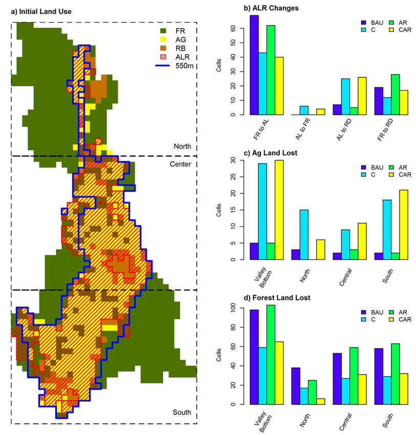
Figure 4 summarizes the impacts of the four scenarios on land within the ALR, land below
550 m elevation, and land in the north, central, and south portions of the watershed. For mapping,
we marked those cells where at least 50% of the cell area is within the ALR as ALR. The last four
delineations are for convenience and illustrative purposes. The elevation cutoff is ‘just right,’ in a
Goldilocks sense, for including forest patches that are embedded in agricultural land and excluding
most forest that is at the interface between agricultural and forested land. The north, center, and south
division is a convenient partition into thirds. For interpreting the results in Figure 4, it is important to
bear in mind that our simulation does not forecast the amount of land-use change that will occur butForests 2019, 10, 581 11 of 20
where a previously decided total amount of land-use change will be located within the confines of
aggregate restrictions such as those imposed for the tested scenarios. Thus, the total amount of land
used for agricultural purposes will increase at the expense of some forested land within the limits of
the restrictions imposed. The total amount of residential and built area in 2050 will be the same
Forests 2019, 10, x FOR PEER REVIEW
in all
12 of 20
scenarios, with the difference being where it is located.
Figure 4. Summary of land-use changes. Land-use types are forest and range (FR), agricultural (AR)
Figure 4. Summary of land-use changes. Land-use types are forest and range (FR), agricultural (AR)
and residential and built (RB). Policy scenarios are business as usual (BAU), forest conservation after
and residential and built (RB). Policy scenarios are business as usual (BAU), forest conservation after
2030
2030(C),
(C),restriction
restriction of
of forest
forest conversion
conversion in in the
theRDCS
RDCSpart
partofofthe
thewatershed
watershed (AR),
(AR), andand both
both forest
forest
conservation
conservation policies together (CAR). ALR refers the Agricultural Land Reserve, and land below 550 m
policies together (CAR). ALR refers the Agricultural Land Reserve, and land below 550
is m
considered valleyvalley
is considered bottom. (a) Map
bottom. (a) of
Mapinitial land uses,
of initial landwith
uses,areas
withofareas
interest identified;
of interest (b) changes
identified; (b) to
land within the ALR; (c) location of loss of agricultural land; (d) location of loss of forest and range
changes to land within the ALR; (c) location of loss of agricultural land; (d) location of loss of forest land.
and range land.
Restrictions on forest land-use change have impacts on the ALR. Land within the ALR does not
need toRestrictions
be used foronagricultural purposes
forest land-use changebut have
have agricultural
impacts on thepotential.
ALR. LandForest and
within therange cells within
ALR does not
the ALRtoinbeFigure
need used 4a
foridentify such purposes
agricultural lands. Conversion
but have of land frompotential.
agricultural forest andForest
range and
within the cells
range ALR to
agriculture
within the within
ALR inthe ALR
Figure 4ahas no impact
identify on total
such lands. land within
Conversion the from
of land ALR.forest
Relative
and to no policy
range within(BAU),
the
the
ALR to agriculture within the ALR has no impact on total land within the ALR. Relative to no policyand
area restriction has little aggregate impact on land in the ALR. The total amount of forest
(BAU),
range the area
inside restriction
the ALR that ishas little aggregate
converted to otherimpact
uses ison land inlower
slightly the ALR.
thanThe total
in the amount
BAU case of forest4b).
(Figure
and range inside the ALR that is converted to other uses is slightly lower than in the BAU case (Figure
4b). However, the portion of forested land within the ALR converted to residential or built is higher.
Forest conservation (C) has the desired effect, reducing the amount of forested land converted to
other uses. However, this increases by approximately four times the amount of agricultural landForests 2019, 10, 581 12 of 20
However, the portion of forested land within the ALR converted to residential or built is higher. Forest
conservation (C) has the desired effect, reducing the amount of forested land converted to other uses.
However, this increases by approximately four times the amount of agricultural land inside the ALR
that is converted to residential and built. Restricting conversion of forested land in one part of the
watershed (AR) shifts the conversion to forested land in the watershed not subject to the restriction.
Restricting conversion of all forested land (C) shifts the conversion to agricultural lands not subject to
the restriction, much of which is in the ALR. Since the ALR was not enforced in the model, the actual
land conversion to residential and built will be lower inside the ALR if the ALR is enforced. In that
case, all land conversion after 2030 would occur in the remainder of the 31 cells that at the start of the
simulation were not the forest and range land-use type and not already built. Prior to 2030, if the ALR is
enforced, much more development will occur on forest and range land than without an enforced ALR.
The policy scenarios that involve protecting forest and range after 2030 drive a large increase in
the conversion of agricultural land, agricultural land that may or may not be in the ALR (Figure 4c).
Most of this occurs in the valley bottom and is conversion from agricultural land to residential and
built. Since residential and built is a collector state, all of the conversion to residential and built is
‘lost’ agricultural land as in the model it will never be converted back to agriculture. In the BAU
scenario there are two more agricultural cells lost than in scenario AR. Two agricultural cells at higher
elevation would have been converted before the end of the simulation if forest and range conversion
in the RDCS was not restricted. The interaction between RDCS forest protection and overall forest
protection after 2030 (CAR) drives development further south and has less impact on agricultural
land in the north. This is a consequence of the spatial association included in our model. We have
documented strong evidence that land-use conversion tends to drive similar land-use conversion
nearby in this watershed [33]. When forest conversion is limited after 2030, there is substantial loss of
agricultural land in the north. When the development of forest land in the north is restricted, it makes
the development of agricultural land less attractive. When AR is in place on its own, no agricultural
land in the north is lost. When C and AR are combined, less than half as much agricultural land is lost
than when C is the only policy. In effect, the AR policy drives development away from agricultural
land in the north by providing less residential and developed cells near agricultural cells to increase
the conversion probability.
Forestry policies also impact forest and range in the valley bottom and affect where lower
watershed changes occur. Figure 4d reports the net amount of forest and range land lost. As can be
noted in Figure 4b, agricultural land is sometimes converted to forest and range land in the model.
However, this reverse conversion is rare in the Okanagan, where climate change is making the land
suitable for a wider variety of crops and population growth and taste trends are together driving an
increase in the demand for locally grown food. One interesting result is that stopping the development
of forest and range land in the RDCS (AR) increases the loss of forest in the valley bottom. While the
effect in the model is small, one cell, it is noteworthy because there is limited forest and range land
in the valley bottom and therefore represents habitat that is particularly important for species that
prefer low elevations and for providing corridors for such organisms to travel between watersheds.
It is also noteworthy that the AR policy increases forest conversion in the central and southern parts of
the watershed. Implementing the AR policy in the RDCS achieves the RDCS objective of protecting
forested land within their jurisdiction. However, from a watershed perspective, it does not protect
forest and range cells. Rather, it drives the conversion to that portion of the watershed not within the
jurisdiction of the RDCS. Protecting forest and range cells throughout the watershed after 2030 reduces
overall conversion out of this land-use type but does not undo the transfer of forest conversion out of
the RDCS area and into other parts of the watershed.
4. Discussion
Landscapes are multifunctional [54]. They provide a variety of services, ranging from the
production of food and fibre through to recreational opportunities and habitat for non-humans.Forests 2019, 10, 581 13 of 20
Managing a multifunctional landscape is challenging, both on account of the complexities inherent
in the interconnections among processes operating on the landscape and on account of the human
agents on the landscape who have a diversity of sometimes conflicting interests in how the landscape
evolves [55–57]. Our modeling exercise highlights the potential for unintended consequences when
chosen policies do not account for the feedbacks whereby an action in one part of the landscape feeds into
decisions elsewhere on the landscape. That these challenges exist is well known [57–60], with [61] an
example where nature protection in one location has effects at other locations. Successfully integrating
them into land-use planning and management has been the challenge [62,63].
The empirical analysis that calibrated our model [33] demonstrated that for this watershed,
distance from a paved road and major urban centers are important predictors of land-use change,
together with an important tendency for conversion to favor land uses that are already present in
neighboring cells (spatial association). These drivers interact with the simple policies halting the
conversion of forest and range land in a portion of the watershed and/or after a particular date to
generate the predicted pattern of land use. These knock on effects lead to potentially undesirable
impacts on socially important landscape functions, food production, and low elevation natural habitat.
Ideally, policy makers would take these interconnections into account and promote the pattern of land
use that best balances the societal value of the landscape functions at a watershed scale. The governance
system makes this challenging.
The governance system is that collection of formal and informal institutions and processes that
together determine how resources will be used and by whom. Governance is fragmented when the
authority is divided between different institutions, which may be multiple local governments within a
watershed and/or multiple senior government agencies with different and possibly conflicting mandates
having authority within the same watershed. The fragmentation of water governance in Canada has
been pointed to as a cause of poor water management outcomes [64]. Globally, this fragmentation is the
dominant pattern when many environmental and resource issues are considered [65]. Fragmentation
makes it challenging for decision makers to coordinate their actions to achieve land-use patterns that
best serve society’s interests. Our results highlight the importance of coordination. If the two regional
governments that span the watershed do not coordinate their policies, then if the RDCS protects
forests within its jurisdiction, this will increase the loss of forest and range land, and agricultural
land, in the area governed by the RDNO. Likewise, if large scale forest protection policies come into
place, likely driven in BC by the Ministry of Forests, Lands, Natural Resource Operations and Rural
Development, our results demonstrate that this will put extra development pressure on agricultural
land, the protection of which is the responsibility of the Agricultural Land Commission. The challenge
posed by governance fragmentation for effective climate change adaptation by agriculture has also
been recognized [66].
Our model results also show that one policy, halting the conversion of forested land in that
part of the watershed within the RDCS, may actually increase the conversion of low elevation forest
elsewhere in the watershed. The Okanagan Valley serves as the only low-elevation, arid corridor
connecting the arid interior of Washington State to the south and the arid south-central interior of
British Columbia [67,68]. Thus, if care is not taken in choosing forest protection policies, protecting
specific parts of the forest in the watershed may reduce the resilience of the ecological systems in
the watershed and even beyond its boundaries. The consultations needed to ensure that the best
combination of landscape functions is sustained need to go well beyond the conventionally considered
interested parties to ensure that all landscape functions are considered.
A maintained assumption in this analysis is that the processes of land-use change, as embodied in
the logistic regression parameters and the underlying biophysical and socioeconomic data, remain the
same over the duration of the simulation. Given that the climate change projections to which these
land-use patterns were to be matched are based on emissions scenarios not coupled to the climate
change projections, the CLUE-S system is the appropriate tool for this analysis. However, the analysisForests 2019, 10, 581 14 of 20
of policy scenarios that cannot be described with area restrictions will require a process-based model
that incorporates the response of decision makers on the land to the policies.
Emphasizing higher density and directing new development towards areas that already have some
development (infill development) would be policies that would reduce the conversion of agricultural
and forest lands to residential and build areas, reducing the magnitude of the changes forecast by our
model. Land-use conversion restrictions may also drive development out of the watershed to areas
where those restrictions are not in place. The province recently introduced a tax on residential units
that are vacant most of the year, as a way of making more rental housing available. This tax was only
applied in the larger and more expensive property markets. There is anecdotal evidence that this is
driving development into nearby communities where the tax is not in place and therefore the cost of
owing residential property is lower. This tax may result in increased the pressure for development in
the study watershed. Payments for ecosystem services may work in the opposite direction, providing
a financial reward for protecting the land in a more natural state. One important extension of this
analysis would be an examination of how incentive-based policies that operate through the land
market can redirect development and/or change its form.
The price for which land trades in a land market is itself a consequence of the uses to which that
land can be put. The value of agricultural land is a derived value, based on the value of the products
that can be grown on the land. The province brought into being the ALR at a time when the profit
land owners could earn farming their land was far less than the profit they could earn by developing
their land. Climate change promises to increase the range of crops that can be grown in the Okanagan,
while potentially leading to declines in other areas. In the future, the price of what can be grown from
the land may serve to reduce the pressure for conversion of agricultural land to residential and built,
while increasing the pressure to convert forested land to agriculture. Extending this work by using a
process-based model can help illustrate how changes in agricultural commodity prices may affect land
uses and water demand.
The importance of markets and incentive-based policies is a consequence of the fact that almost
all of the agricultural and build land area in the watershed is private property, as is some of the lower
elevation forested land. Halting land conversion on public lands is relatively easy, when contrasted
with halting land conversion on private lands. Private land owners typically have the right to do
anything they would like to do with their land, provided there are no clear and traceable adverse
impacts on other land owners or the public at large. Policies that directly mandate the use that private
owners can make of their land are strongly resisted, leaving such command and control policies
to situations where the adverse impacts of particular uses are obvious and strongly detrimental.
Such was the case in the implementation of the ALR to restrict rapid conversion of the scarce provincial
agricultural land base. Most policies must therefore rely on persuasion, either moral suasion or through
incentive-based policies, such as payments for ecosystem services [69–73]. The policy must make
that land use which is best for society be that one which is preferred by the private land owner [74].
Our analysis provides an ‘as if’ analysis, as if land-use restrictions could be effectively implemented.
Those proposed are reasonable to assume for that part of the restricted land that is publically owned,
which for our case watershed is most of the restricted land.
A few directions for future work are suggested by this discussion. Where CLUE-S is a pattern-based
land-use change model, alternative process-based systems, often agent-based systems, focus more
explicitly on the agent making the land-use choice [75,76]. Moving in this direction is consistent
with continuing calls to better integrate human behavior into coupled human-environmental systems
analysis [77–80]. Where the current land-use change is based on transition probabilities informed by the
observed pattern of land use, in an agent-based land-use change model, land use is chosen by a model
agent, in response to changes in those things that impact the agent’s objective. Incentive-based policies
and market mediated influences can thereby be incorporated into the model and their consequences
observed (as suggested in [81]).Forests 2019, 10, 581 15 of 20
Our analysis does not explicitly evaluate ‘best’ patterns of land use. Doing so would require
making judgements about the relative values of different functions provided by the landscape. It would
be possible to assign a value reflecting the services provided by each cell in the simulation, based on the
land use in that cell. These values could then be aggregated for each scenarios, and then the scenarios
can be ranked [82–84]. The source of these values is the challenge with such an approach, as the choice
of the values will determine which policy scenario is ranked highest. Engaging communities with
the ranking or valuation of these landscape functions is receiving attention in this area and could be
pursued as an application of these results [62,63,85].
The identified challenge of governance fragmentation suggests that future work would be more
valuable if it is undertaken more collaboratively with those that would use and be impacted by the
results [86]. An agent-based approach lends itself to participatory model building in a way that
pattern-based systems like CLUE-S do not [78,87]. Engaging local government, staff from provincial
and federal ministries, and land users with the process of building the land-use change model builds an
appreciation of the complex interactions that are at play, and fosters a sense of ownership of the model
and therefore an acceptance of the results [88,89]. We expect the results of the current project can serve
as a starting point for a conversation about the complexities involved in managing a multifunctional
landscape and building both tools and relationships that can improve the quality of this management.
5. Conclusions
The Okanagan Valley has seen continuing rapid population growth for several decades, growth
which is likely to continue. The challenge is finding that pattern of land use which best reflects the
value that society places on the multiple functions provided by the landscape and then figuring out
how to achieve this best pattern. We have herein reported on the use of a land-use change forecasting
system to explore how land use is likely to change in the Deep Creek sub-basin of the Okanagan
Valley under four different forest conservation policy scenarios. Our results demonstrate that failing to
consider the multifunctional nature of the landscape when implementing policies can have unintended
consequences. In this case, protecting forest land drives development onto agricultural land and may
hasten the loss of low elevation forest. With provincial food sovereignty and enabling ecosystem
adaptation to climate change of importance to the provincial population, the best form of the landscape
will balance these functions with those provided by forest alone.
Bringing results like these into the decision-making process can be frustrated by the fragmentation
of land-use governance. The pervasiveness of externalities requires considering the impacts of decisions
beyond individual land owners and local communities. However, delegation of authority without
processes to ensure coordination can lead to decisions that do not reflect the complexity of the system.
Good land-use management therefore requires integrating knowledge and reflecting values from
multiple affected communities. Recent innovations in land-use planning technologies and processes
hold the promise to transform land-use planning into a process that builds collaboration and enables
better coordination. Decision makers at all levels should actively pursue these new approaches to
land-use planning.
Author Contributions: Conceptualization, M.A., J.J., C.N., and A.W.; methodology, M.A.; software, M.A.;
validation, M.A.; formal analysis, M.A. and J.J.; writing—original draft preparation, M.A.; writing—review and
editing, J.J. and C.N.; visualization, M.A. and J.J.; funding acquisition, A.W.
Funding: This research was funded by the Canadian Natural Science and Engineering Research Council and the
University of British Columbia.
Acknowledgments: We are grateful to local government staff who reviewed and commented on our results.
Conflicts of Interest: The authors declare no conflicts of interest. The funders had no role in the design of the
study; in the collection, analyses, or interpretation of data; in the writing of the manuscript; or in the decision to
publish the results.You can also read