Bronson Creek An Integrated Study of an Urban Stream in Washington Co., Oregon - Paula Hood
←
→
Page content transcription
If your browser does not render page correctly, please read the page content below
Bronson Creek
An Integrated Study of an Urban Stream in Washington Co., Oregon

                          Paula Hood
                        December 8, 2008
INTRODUCTION

       The flow of water through an undisturbed watershed is a complex process. Precipitation

percolates into the ground, saturating the soils by filling the spaces between soil particles. Water

moves very slowly through the soil as groundwater, eventually recharging streams and rivers even in

times of low precipitation or drought. Water is also taken up and stored by trees, fungi, rotting logs,

and other plant and animal life. Some water evaporates and enters the atmosphere, and later falls back

to earth as precipitation. Streams and rivers transport the water out to the oceans, where it becomes

part of the cycle of the world’s weather patterns and precipitation. In many steps along its way through

a watershed, water is filtered, cooled, and distributed slowly over the landscape to create a diversity of

plant life, wildlife habitats, and ecosystems (Caduto 1990; Murdoch 2001; Robertson 2008).

       In urban watersheds, however, the historic patterns of water movement, filtration, and

distribution across the watershed are disrupted, potentially causing a variety of problems. Human

developments such as shopping malls, neighborhoods, condominiums, gas stations, roads, and parking

lots all have impacts on water movement and water quality. Large areas of impermeable surfaces (such

as concrete parking lots and roads) cause water to be transported quickly into streams, rather than

percolating into the soil and eventually the ground water. This takes away important filtration and

cooling mechanisms, and the run-off water can pollute streams with petrochemicals and residues from

leaking cars, as well as cause stream temperatures to rise significantly, particularly during the summer

months when pavement is hot. Run-off water from urban areas can pick up and transport other

pollutants into streams as well. Typical non-point source pollutants in an urban watershed also include

fertilizers, pesticides, and herbicides from gardens and small farms, fecal bacteria from dogs, cats, and

faulty septic systems, toxic pollution from factories and residential spills, and excess sediment from

construction, roads, and erosion. With ever-expanding urban and suburban developments, agriculture,

                                                                                                          1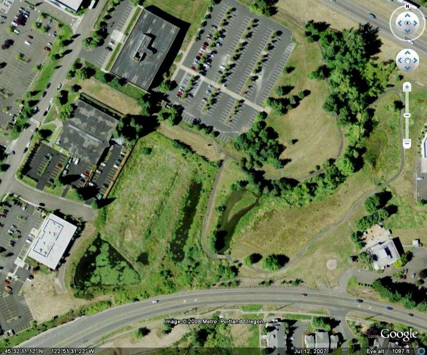
and resource extraction, streams face many different challenges to their health, and to their ability to

support a diversity of fish and wildlife (Murdoch 2001; Robertson 2008).

       Vegetation (particularly riparian vegetation), stream structure, and soils, all play large roles in

protecting the overall biotic integrity of the streams in a watershed. In urban watersheds, streams are

often heavily channelized to make room for human development. Complex stream structures such as

meanders, natural wetlands, side channels, and flood plains are severely limited or non-existent.

Levees, rip-rap, and culverts are used to constrain streams to more narrow channels in order to direct

them under roads and between developments. This changes their structure and their historic flow

patterns, often causing them to widen and slow in certain areas (particularly around culverts), which

can raise water temperature beyond acceptable levels. Many stream organisms such as certain

macroinvertebrate species and fish (including salmonids) rely heavily on complex structural habitats

such as pools, riffles, cut-banks, and side channels. Complex stream structure is a key component of

the biotic integrity of a stream, and many aquatic organisms can not survive without the conditions

found in these habitats (Murdoch 2001; Robertson 2008).

       Limited riparian vegetation in an urban watershed can be a major source of concern. Because

of the importance of riparian vegetation, looking at the land and the vegetation surrounding a stream is

a good place to start when beginning an inquiry about a particular stream’s health. Riparian vegetation

provides many important functions for a stream. The overhanging vegetation shades the stream,

keeping water temperatures cool. (Murdoch, et al. 2001; Voshell 2002) Many of the organisms that

live in a stream may not be able to tolerate warm water. Some species of fish and many species of

macroinvertebrates, for example, need cooler water temperatures in order to survive (Adams 2003).

Even the comparatively small shade provided by overhanging grasses can make a crucial difference in

stream temperature (Caduto 1990; Voshell 2002). Riparian vegetation serves to support a reliable flow

of ground water, even in low rain-fall seasons, because the roots of the vegetation keep soil from being

                                                                                                             2
compacted, and promote soil pores which can hold ground water. Plant roots also hold soil in place,

preventing erosion of sediment into the stream. Erosion of stream banks can introduce large and

continuous amounts of sediment, negatively impacting macroinvertebrates, fish, and amphibians.

Riparian vegetation also provides protective cover and nursery habitat for spawning and young stream

organisms. Grassy backwaters, protected weedy areas, and pools formed by large downed wood are all

important examples of essential rearing and spawning habitats formed by the presence of riparian

vegetation (Caduto1990; Murdoch 2001; Robertson 2008; Voshell 2002).

       A watershed’s soil is very important to the overall health of the watershed, and particularly to

the health of the streams in the watershed. The soils in a watershed are a product of several factors,

including the geology of the area, topography, climate, and vegetation. The composition of the soil

parent material is important to soil structure and characteristics, and can be made up of materials such

as bed rock, ash from volcanic eruptions, or fine silts from great floods (Robertson 2008). Vegetation

has important influences on soil characteristics and health. Soils, and all of the organisms living in

those soils, are important for recycling and releasing nutrients in the system. Plants and other

organisms depend on these nutrients, such as nitrogen, that are converted into usable forms by soil

biota. The healthier the soil, the greater its ability to support healthy and diverse animal, plant,

bacterial, and fungal communities. Without healthy soils, erosion, compaction, poor plant growth, and

compromised ecosystems all affect the watershed and its streams (Robertson 2008).

       Because activities which take place in one part of a watershed can drastically affect another

area, sometimes miles away, stream water quality can be an effective indicator of problems over large

areas. For example, if substantial percentages of a watershed have been deforested and replaced with

impermeable concrete surfaces then, as a result, higher-than-historic water temperatures may be a

problem many miles downstream of the deforested area. Another example is when sediment,

pesticides, and toxic pollution are picked up from the land by rainwater run-off, bringing it into nearby

                                                                                                           3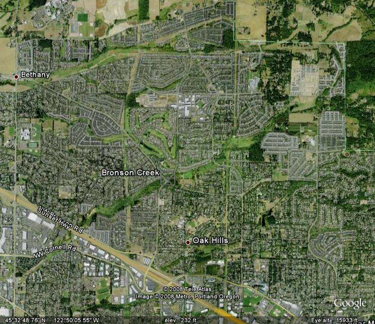
streams both small and large. Those streams carry the pollution to larger streams, and then those

streams carry it to even larger streams, and so on. Examining a small section of stream can be an

effective way to assess the health of the watershed upstream of the sample site. (Murdoch 2001). On a

finer scale, investigating the riparian vegetation adjacent to a relatively small stretch of stream is

important, too. Even a relatively small stretch of stream with adequate riparian vegetation, natural

curvature, and complex structure can make a positive difference to a larger area, especially in an urban

area. Urban conservation and restorations projects often focus on relatively small available stretches of

streams or wetlands. While these preserved or restored areas may not be very large, the services they

provide are very tangible and include flood control, temperature control, filtration of pollution,

wildlife and fish habitat, providing clean oxygen, CO2 sequestering, recreation, and a higher quality of

life for humans near and far (Adams 2003; Murdoch 2001).

       The Clean Water Act (CWA) was created to require protection of water quality for beneficial

uses, including recreation and wildlife habitat. The Endangered Species Act (ESA) mandated

protection of species listed as endangered or threatened. The CWA necessitated the creation of criteria

and standards for water quality. Many government agencies and groups work together to ensure that a

balance between human uses and environmental quality is reached, and that water quality standards

are met. When water quality standards are not met, improvement plans and monitoring are put in place

to ensure movement towards the attainment of water quality standards. Particularly in areas with

endangered or threatened species such as certain salmonids, water quality standards may be based on

the recovery or health of these species (Smith et. al. 2005).

       Our study assessed the general character and health of Bronson Creek, an urban stream in

Washington County, Oregon. We collected data on stream curvature, stream discharge, riparian

vegetation, chemical water quality parameters, and macroinvertebrate populations along a small

stretch of Bronson Creek. General watershed health was also taken into account, and we looked at

                                                                                                         4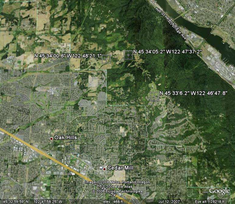
some of the land uses and potential problems in the drainage as a whole. These parameters

encompassed the five components of stream biotic integrity: habitat structure, water quality, energy

source, and flow regime, and biotic interactions, and provided for a holistic approach in looking at the

stream’s health (Murdoch 2001). Studying all of these parameters is important in helping to determine

the conditions within a stream, such as whether there is enough oxygen for aquatic organisms,

including salmonids, to survive. Monitoring these parameters is also important in making sure that a

stream is in compliance with the Clean Water and Endangered Species Acts. Water from Bronson

Creek flows into Beaverton Creek and Rock Creek, and then eventually into the Tualatin River. The

Tualatin River supports salmonids and other species which are legally protected under the Endangered

Species Act. Historically, Bronson Creek, Beaverton Creek, and Rock Creek may have supported

steelhead or other salmonid species (Robertson 2008; Smith et. al. 2005). Bronson Creek has had

documented problems meeting water quality guidelines, often exceeding standards for pollutants such

as bacteria and high temperatures (EPA 2008; Smith et. al. 2005) This study allowed us to determine

some of the challenges facing Bronson Creek, the possible sources of those problems, and restoration

opportunities to improve the creek.

METHODS AND MATERIALS

BRONSON CREEK LOCATION, BACKGROUND, and HISTORY

       Bronson Creek is a small stream located almost entirely within Washington County, Oregon

(figure 1). The headwaters flow from the Forest Park area in Multnomah County, and most of the

stream reach is not more than a few miles outside of Multnomah County and the Portland city limits.

From its headwaters in the top of Forest Park and the Tualatin Mountains, the stream flows southwest

until it drains into Beaverton Creek, which is a tributary of Rock Creek. In turn, Rock Creek flows into

the Tualatin River, which eventually drains into the Willamette River. The mainstem of Bronson

Creek is approximately 5 miles long, and flows under several major roads, including Laidlaw, Kaiser,

                                                                                                       5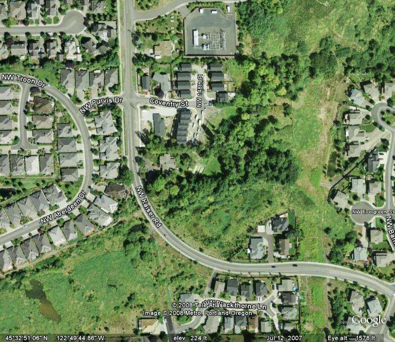
West Union, Hwy 26, and Cornell Blvd (figure 3) (Delmore, 2004; Robertson, 2008). The creek is also

adjacent to major urban developments, such as Tannesborne Mall, large parking lots, apartments,

condominiums, and new construction (Robertson, 2008).

FIGURE 1: Oregon Counties, with Washington County highlighted
Copied from: commons.wikimedia.org:

                      FIGURE 2: Watersheds within the Tualatin River Basin
   Image copied from: http://www.swrp.esr.pdx.edu/images/watersheds/maps/tualatin_basin.jpg
                                                                                                  6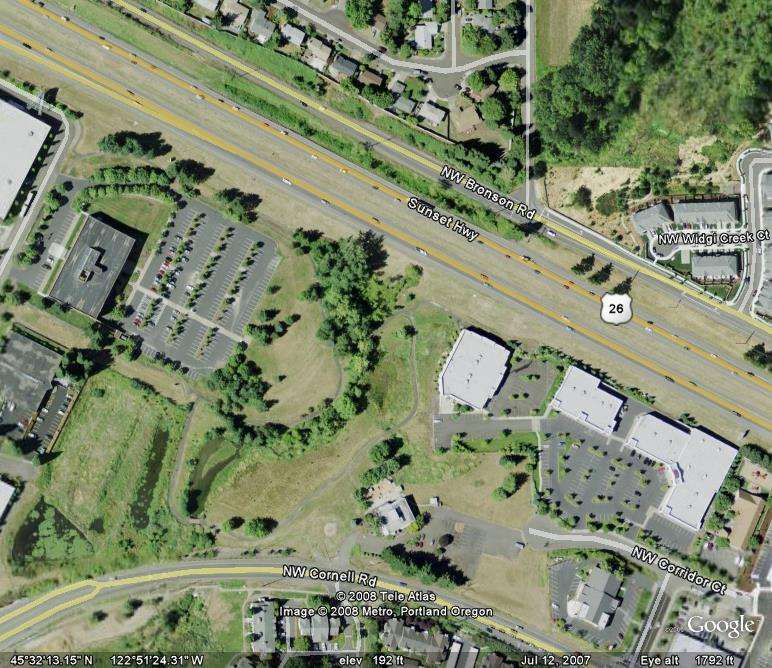
Tualatin Mountains
Bronson Creek
Headwaters
Bronson Creek
Study Site
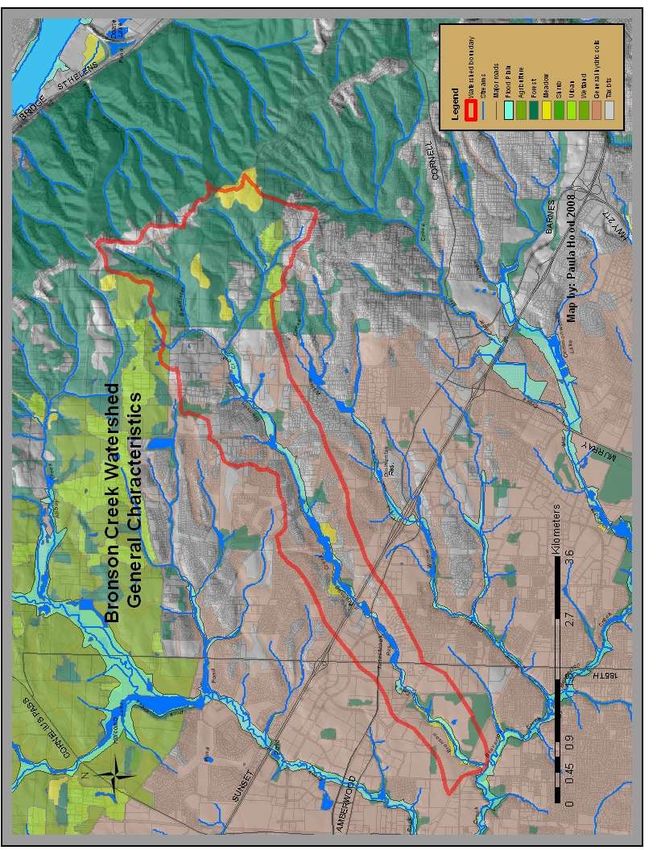
FIGURE 3: Bronson Creek. Satellite image copied from: Google Earth
7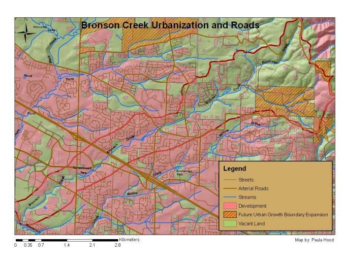
Bronson Creek

          Storm Water Retention
          Pond and Wetland

FIGURE 4: Main study reach of Bronson Creek
Adapted from a GoogleEarth picture copied from Dr. Robertson’s ESR202 lecture notes, 2008.

       By the mid 1800’s, European settlement had dramatically changed the Tualatin River basin,

including Bronson Creek watershed. Previous to European settlement, native peoples living in the

Tualatin River basin had survived by hunting big game animals and gathering berries, Wapato, camas,

and other native plants. They used controlled burns to promote some of these resources on the

landscape (Smith et. al. 2005). As Europeans arrived, the landscape was altered by logging, trapping,

and agriculture, and eventually by roads, cities, and urbanization. Streams were particularly impacted

by damming, removal of large woody debris, irrigation, channelization, and pollution. By the 1970’s,

the need for healthier streams and tighter regulations had been recognized. The Clean Water Act

(CWA) was created to require protection of water quality for beneficial uses, including recreation and
                                                                                                         8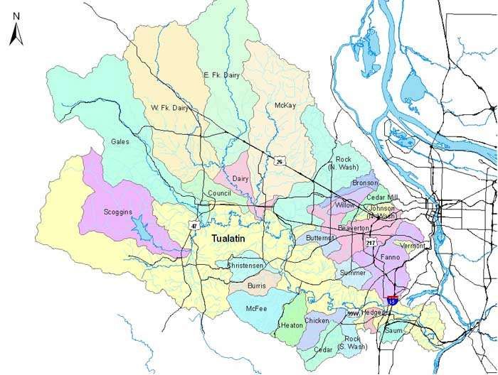
wildlife habitat. The Endangered Species Act (ESA) mandated protection of species listed as

endangered or threatened, including recovery plans for their long-term survival (Robertson 2008;

Smith et. al. 2005).

       Today, Clean Water Services (CWS) has jurisdiction over streams and surface water within the

Washington County urban growth boundary, including Bronson Creek. The goals, regulations, and

mission of the agency are driven primarily by the CWA and the ESA. Part of the mission of the CWS

is to “provide cost effective and environmentally sensitive management of resources” (Smith et. al.

2005). In order to fulfill these goals, the CWS created the Healthy Streams Plan, which includes all

streams within the urban portions of the Tualatin basin, as well as some stream reaches beyond the

urban boundary which flow into the urban boundary. Bronson creek is included in the Healthy Streams

Plan. CWS has been monitoring Bronson Creek since 1994, and developing restoration projects since

1998. A major thrust of the Healthy Streams Plan is to move streams in the Tualatin basin towards

meeting the standards of the CWA and the ESA in the Tualatin Basin. Not all streams in the basin

currently meet water quality standards. The Healthy Streams Plan is designed to go beyond meeting

the standards set in place because of the CWA and the ESA and instead set broad goals that include

sustainable use strategies and planning for the future as well (Smith et. al. 2005).

       The Tualatin River basin currently supports steelhead, coho, Chinook, cutthroat trout, and

rainbow trout, and Pacific lamprey, as well as other less sensitive fish species (Smith et. al. 2005). The

cutthroat trout are not anadromous (VanderPlaat 2003). Winter steelhead and spring Chinook are listed

as threatened species under the ESA (Smith et. al. 2003)). Pacific lamprey were petitioned for Federal

Listing in 2003, and the decision is pending (VanderPlaat 2003). According to the Technical

Memorandum: Biological Basis for Fish Passage at Scoggins Dam, Coho and Chinook are not native

to the Tualatin River basin, and were introduced in the early 1900’s (VanderPlaat 2003). Conflicting

data exists for which salmonid species currently exist or historically may have existed in Bronson

                                                                                                         9
Creek, Beaverton Creek, and Rock Creek. According to streamnet, Rock Creek supports cutthroat
trout, rainbow trout, and lamprey (streamnet 2001). According to an EPA document, Rock Creek also
supports steelhead and Coho (EPA). Streamnet lists sensitive species in Beaverton Creek to be
cutthroat trout and Pacific lamprey (streamnet 2001). Bronson Creek, according to the Tualatin River
Subbasin TMDL- Appendix F (Fish Habitat), has cutthroat trout present (EPA), but according to
streamnet it does not (streamnet 2001). An online Metro document states that: [t]hreatened species
such as steelhead, cutthroat trout and Coho salmon are present in Rock, Abbey, Holcomb, Bannister,
and Bronson creeks, as well as in an Abbey Creek tributary” (Metro Regional Government 2007).
Taking the data together, it seems reasonable to say that resident cutthroat trout may have been
the most likely to reach into Bronson and Beaverton Creeks, and may still inhabit Rock Creek. Pacific
lamprey occur in Bronson and Beaverton Creeks. Rock Creek may still support steelhead. Pacific
lamprey occur in Beaverton Creek and Bronson Creek. It is possible that Beaverton and Bronson
Creeks may have historically supported steelhead, but it is not clear whether or not this was actually
the case.
At least 25 different restoration and enhancement projects are being coordinated by CWS in
the Tualatin basin. One of the main general stream restoration goals across the Tualatin Basin is to
increase stream base flows, as most are lower than historic levels. Also, CWS mandated that beaver
trapping be stopped, and beaver have returned to the landscape (Smith et. al. 2005).
Bronson creek is identified as high priority watershed for fish and water quality. Much
restoration has already been done on Bronson creek, including revegetation, addition and placement of
large woody debris, fish barrier removal, livestock exclusion, and pond modification. Modification
and partial removal of the Tannasbrook ponds has already been completed. The Tannasbrook ponds
were created in the1950s by impounding Bronson Creek, just south of Cornell. The ponds caused
problems with high temperatures and low dissolved oxygen. Dissolved oxygen was sometimes as low
10as 1-3mg/L. Extensive cooperative effort was made between CWS, private home owners, apartment
complex owners, and businesses in order to form the restoration plan. Other restoration work has also
been completed or partially completed along Bronson Creek. The estimated costs of the enhancement
projects along Bronson Creek are $1,295,000 (Smith et. al. 2005)
11FIGURE 5: Bronson Creek watershed, general characteristics.
12FIGURE 6: Bronson Creek Urbanization and Roads
METHODS AND MATERIALS I
STRUCTURE AND VEGETATION
To study the riparian vegetation in the small stretch of Bronson Creek, we mapped the
contours of the stream and the vegetation along the stream, and we recorded the dominant plant
species and percentage of vegetation cover. Our survey team mapped a 150 meter section of Bronson
Creek between Hwy 26 and Cornell Blvd. We first mapped the stream contours, using the baseline
method. We laid the baseline and the transects using landmarks. The baseline was run along the south
side of the stream, at 311 degrees facing northeast. Transects were run every 10 meters off of our 150
meter baseline. Transects were laid at a 90 degree angle to the baseline using a compass. In order to
13map the vegetation, we used the Modified Line Intercept Method, which is a mixture of several
methods and included the use of a spherical densitometer (Spherical Densiometer, Inc). We followed
the baseline and the transects we had run for mapping the stream contours. Walking along each
transect, we recorded the general type of vegetation present, and the length of that vegetation type
along the transect. Vegetation was classified as one of the following types: wet meadow, emergent
wetland, or woody riparian. We also recorded, for one meter on either side of the transect, the percent
coverage of the types of ground cover along the transect within each of these areas. The ground cover
types were divided into forbs, rushes, grasses, and sedges. We recorded any tree or shrub within 2
meters on either side of the transect. We identified and recorded the taxa of the trees and shrubs, and
measured the circumference of any tree or shrub over approximately 20cm in diameter. Finally, we
used a spherical densitometer to estimate canopy cover in each different vegetation type that the
transect crossed (wet meadow, emergent wetland, or woody riparian). Canopy cover was measured
with the densitometer in approximately the middle of each vegetation type along the transect. The data
we collected was analyzed using Microsoft Excel (Microsoft Corporation, 2003).
WATER QUALITY AND STREAM DISCHARGE
The water quality and chemical parameters we studied were pH, dissolved oxygen, CO2,
temperature, specific conductivity, total dissolved solids, turbidity, dissolved nitrogen, dissolved
phosphorus, total hardness, silica, oxygen reduction potential, and discharge. Water quality chemical
tests and stream discharge readings were taken once a week for 3 weeks, on 10/08/08, 10/15/08, and
10/22/08. The measurements were taken at approximately 3pm on each of these days. The water
quality parameters that were measured using the YSI Quality Meter (YSI Corporation) were:
temperature (in degrees Celsius), dissolved oxygen (both in percent saturation and parts per million),
specific conductivity (in micro siemens per cm), total dissolved solids (in parts per thousand), pH, and
14oxidation reduction potential (in millivolts). Temperature was also measured hourly at five sites from
September 26th through November 4th using temperature mini-log probes (Vemco, Inc.). Turbidity was
recorded in NTU’s using a Turbidimeter (Orbeco-Hellige Inc.). Other chemical water quality
measurements were taken using LaMotte field water chemistry kits (LaMotte Corporation). Those
chemical parameters were dissolved silica (in milligrams per liter), pH, dissolved oxygen (in
milligrams per liter), total hardness (in milligrams per liter), dissolved nitrogen (in milligrams per
liter), dissolved phosphorous (in milligrams per liter), and carbon dioxide (in milligrams per liter). To
measure the water velocity of the stream, we used a stream water velocity meter (Swoffer Inc), which
measured the stream velocity in meters per second. The data from the water quality and discharge
parameters was analyzed using Microsoft Excel (Microsoft Corporation, 2003).
On each of the three days, the chemical water quality parameters taken with the YSI were
measured at each of the 6 sampling sites in our stream reach (figure 7). The 6 sites included “Site 1”
(below HWY 26), “Site 2” (in the wooded riparian area near the large ash tree), “Site 3” (on the north
side of the large pool in our study reach), “Site 4” (near the lower foot bridge), “Site 5” (just north of
Cornell Blvd.), and “Site 6” (at the wetland outlet just north of Cornell Blvd.). The chemical water
quality parameters measured using the LaMotte field water chemistry kits were taken at 4 sites on each
of the 3 days. Turbidity was taken at each of these sites as well. These sites included the site near
HWY 26, the site just north of Cornell Blvd, the wetland outlet, and the woody riparian area south of
HWY 26, close to the ash tree. The stream velocity, depth, and width were measured at 2 sites on each
of the 3 days, near HWY 26, and near Cornell.
15Stream Discharge
YSI
Water Quality
Kits
Invertebrates
Stream Discharge
FIGURE 7: Bronson Creek study reach, water quality, stream discharge, and invertebrate sampling sites.
Adapted from a GoogleEarth photo copied from Dr. Robertson’s ESR202 lecture notes, 2008.
FIGURE 8: Bronson Creek
Copied from Dr. Robertson’s ESR202 lecture notes, 2008.
16MACROINVERTEBRATES
Macroinvertebrates were sampled once a week for 3 weeks, on 10/08/08, 10/15/08, and
10/22/08, at four sample sites within the stream study reach. The samples were taken between
approximately 3pm and 4:30pm on each of these days (figure 7). The invertebrates were sampled
using dip nets (Ward’s Biological Supply Co.), kick nets that meet EPA standards (Ward’s Biological
Supply Co.), and Surber samplers (Ward’s Biological Supply Co.). Invertebrates were sampled for
approximately the same amount of time at each site. All of the invertebrates in the samples were
preserved in 70 percent Ethanol in small jars. Invertebrate samples were then analyzed using the
sequential comparison index and diversity index (Brower et. al. 1998) and the pollution tolerance
index (Murdoch and Cheo 1996).
WATERSHED TOUR
On 11/05/08 we took a watershed tour along the Bronson Creek watershed, driving to the
upper reaches of the watershed and stopping at 6 sites above our study reach, and then 3 more within
our study reach. We took topographic maps of the Bronson Creek watershed, cameras, and GPS units.
We also used the YSI and the turbidimeter, and took data readings at some of the stops (figures 30 and
48). Geographic Information System (GIS) maps were created using ArcMap (ESRI 2007).
RESULTS
STREAM STRUCTURE AND VEGETATION
STREAM STUCTURE
The physical layout of Bronson Creek in the 150 meter study stretch between Hwy 26 and
Cornell is characterized by varying widths of the stream channel, ranging from almost 25meters across
to barely 2 meters across. The average width is 9.4 meters. The downstream third of the stream, the
stretch near the wooden bridge and towards Cornell road, was the widest and most open, with the
17fewest trees present. The upper third of the stream, towards Hwy 26, on the north side of the stream
had the most trees and the thickest canopy cover. The stream itself is fairly straight and channeled,
particularly when compared to the historic floodplain around the stream, which has been extensively
built upon. However, some curvature does exist to the stream, and in this section the curves stretch
over an approximately 40 meter width. Along the north side, for example, the curves reach from, at
minimum, just less than 12 meters away from the baseline to, at maximum, 54 meters away from the
baseline.
Bronson Creek
60
distance from baseline, m
50
40
30
20
10
0
0 50 100 150
Baseline, in meters
FIGURE 9: The basic outline of the stream contours along our study reach.
VEGETATION
The riparian vegetation along Bronson Creek is dominated by emergent wetland with 2170
square meters. Across the study reach, wet meadow covers an area of 1939.2 square meters. Forested
riparian covered the least area in the study site, occupying only 824 square meters. It is useful to look
at the study area in thirds, because each of the 3 portions of streams is fairly distinct from each other.
In the first section (0 to 60 meters, starting from downstream on the baseline), the wet meadow
18predominates, and grasses were the dominant plant in the wet meadows. In the second section (60 to
100 meters), emergent wetland dominates, with a mix of grasses (reed canary grass and others),
sedges, rushes, shrubs (such a Himalayan blackberry, willow, Douglas spirea, and Pacific ninebark),
and small trees (such as ash, oak, red alder, and red twig dogwood). In the third section, forested
riparian covers the most area, followed very closely with emergent wetland and then wet meadow. The
forested riparian area was dominated by medium and large trees (such as European alders, ash, Oregon
ash, and Douglas hawthorn). The shrub Himalayan blackberry also co-dominated in some areas of the
forested riparian (Pojar and Mackinnon 2004, Lien 2008). (For a detailed list of tree and shrub taxa
recorded at each site, see APPENDIX A at the end of this report.)
FIGURE 10: Bronson Creek study reach, contours plus vegetation types.
Figure by Cheryl Conway, ESR202, 2008.
19Bronson Creek Vegetation Types
(All sections)
22%
37%
wet meadow
emergent wetland
forested riparian
41%
FIGURE 11: Composition of the riparian vegetation in the study reach.
Bronson Creek Vegetation Types
1200
Area in square meters
1000
800
wet meadow
600 emergent wetland
forested riparian
400
200
0
section one section two section three
FIGURE 12: Dominant vegetation types in each section of the study area.
20Bronson Creek Ground Cover
(percentage, all sections)
0.3 4.8
12.5
2.2
82.2
forbs
rushes
grasses
sedges
other
FIGURE 13: Ground Cover percentages across all sections. The “other” in the chart refers to bare
ground, or ground area covered by trees or shrubs.
Grasses dominated as the ground cover in all vegetation types and in all sections. Rushes and
sedges were small percentages both overall and in any one area, Grasses dominated as the ground
cover in all vegetation types and in all sections. Rushes and sedges were small percentages both
overall and in any one area, and forbs as ground cover were rare.
Bronson Creek Ground Cover
(section 1, low er third)
120
percent coverage
100 forbs
80 rushes
60 grasses
40 sedges
20 other
0
w et emergent forest
meadow w etland riparian
FIGURE 14: Ground cover composition in the first stream section (the section closest to Cornell
Blvd.) according to each vegetation type.
21Bronson Creek Ground Cover
(section 2, m iddle third)
100
percent coverage
80 forbs
rushes
60
grasses
40
sedges
20
other
0
w et emergent forest
meadow w etland riparian
FIGURE 15: Ground cover composition in the second stream section (the middle section) according
to each vegetation type.
Bronson Creek Ground Cover
(third section, upper third)
100
percent coverage
80 forbs
rushes
60
grasses
40
sedges
20
other
0
w et emergent forest
meadow w etland riparian
FIGURE 16: Ground cover composition in the third stream section (the section closest to HWY 26)
according to each vegetation type.
22Average Canopy Cover Present for
each Vegetation Type
(all sections)
9.23
21.7 wet meadow
emergent wetland
60.6
forest riparian
FIGURE 17: Represents the average canopy cover for each vegetation type over the entire study area.
Bronson Creek Canopy Cover w ithin Distict
Vegetation Types (section 1, low er third)
percent canopy cover
100
80
60
40 canopy cover
20
0
w et emergent forest
meadow w etland riparian
FIGURE 18: Represents the average canopy cover for each type of vegetation in the first stream
section (closest to Cornell Blvd.).
Bronson Creek Canopy Cover w ithin Distinct
Vegetation Types (section 2, m iddle third)
percent canopy
100
80
coverage
60
canopy cover
40
20
0
w et emergent forest
meadow w etland riparian
FIGURE 19: Represents the average canopy cover for each type of vegetation in the middle stream
section.
23Bronson Creek Canopy Cover w ithin Distinct
Vegetation Types (section 3, upper third)
percent canopy
100
80
coverage
60
40 canopy cover
20
0
w et emergent forest
meadow w etland riparian
FIGURE 20: Represents the average canopy cover for each type of vegetation in the third stream
section (closest to HWY 26).
CHEMICAL WATER QUALITY
The highest fluctuations in temperature on a daily basis were seen at the Cornell sampling site,
one of the 5 locations where hourly temperatures were taken using the temperature probes. The
Cornell site also reached the highest temperatures, up to 19.4 degrees Celsius. The daily temperature
fluctuated as much as 7.4 degrees at the Cornell Site, with an average fluctuation of 4 degrees. Other
sites did not fluctuate as greatly, nor hit the same high temperatures. The highest temperature reached
at HWY 26, for example, was 14 degrees. The largest fluctuation the HWY 26 site saw over a day was
2.1 degrees Celsius. The average amount the daily temperature fluctuated was 0.9 degrees. The Kaiser
site also had very little temperature fluctuation compared to the Cornell site, and like the HWY 26 site,
tended to remain cooler during the day hours and warmer during the night and early morning hours
than did the Cornell site. The Bethany and Laidlaw sites did not fluctuate as much as the Cornell site
did, but more than the Kaiser and HWY 26 sites. Laidlaw and Bethany were almost always warmer
throughout the entire day than either Kaiser or HWY 26. Particularly during the period from October
29th to November 5th, Laidlaw had the highest temperatures of any of the sites, surpassed only briefly
on two days by the Cornell site. During the time periods of October 4th through October 6th and
24November 3rd through November 5th, Cornell did not fluctuate as widely as it did during the rest of the
sample time period. Air temperatures fluctuated more widely than any of the stream temperatures over
the study period, reaching both higher and lower temperatures than all streams on a daily basis.
(See APPENDIX B for a comparison of hourly temperature data for the Cornell, HWY 26, and Kaiser
sites in Bronson Creek.)
Hourly Temperature Data for Bronson Creek
Five Sites Compared
22
20
Tempertature, Degrees Celsius
18
16
14 Cornell
12 Laidlaw
Kaiser
10
Bethany
8 HWY 26
6
4
2
0
8
8
8
8
8
8
8
8
8
8
8
8
8
00
00
00
00
00
00
00
00
00
00
00
00
00
-2
-2
-2
-2
-2
-2
-2
-2
-2
-2
-2
-2
-2
09
09
09
09
09
09
09
09
09
09
09
09
09
-
-
-
-
-
-
-
-
-
-
-
-
-
26
27
27
27
28
28
28
29
29
29
30
30
30
September 26th - 30th
FIGURE 21: Hourly temperature data for Bronson Creek for all five temperature probe sites from
September 26th through September 30th.
25Hourly Temperature Data for Bronson Creek
Five Sites Compared
22
20
Temperature, Degrees Celsius
18
16
14 Cornell
12 Laidlaw
Kaiser
10
Bethany
8
HWY 26
6
4
2
0
8
8
8
8
8
8
8
8
8
8
8
8
8
8
8
8
8
8
8
8
8
/0
/0
/0
/0
/0
/0
/0
/0
/0
/0
/0
/0
/0
/0
/0
/0
/0
/0
/0
/0
/0
0
0
0
0
0
0
0
0
0
0
0
0
0
0
0
0
0
0
0
0
0
/1
/1
/1
/1
/1
/1
/1
/1
/1
/1
/1
/1
/1
/1
/1
/1
/1
/1
/1
/1
/1
01
01
01
02
02
02
03
03
03
04
04
04
05
05
05
06
06
06
07
07
07
October 1st - 7th
FIGURE 22: Hourly temperature data for Bronson Creek for all five temperature probe sites from
October 1st through October 7th.
Hourly Temperature Data for Bronson Creek
Five Sites Compared
22
20
Temperature, Degrees Celsius
18
16
14 Cornell
Laidlaw
12
Kaiser
10
Bethany
8
HWY 26
6
4
2
0
08
08
08
08
08
08
8
8
8
8
8
8
8
8
8
8
8
8
8
8
8
/0
/0
/0
/0
/0
/0
/0
/0
/0
/0
/0
/0
/0
/0
/0
0
0
0
0
0
0
0
0
0
0
0
0
0
0
0
0
0
0
0
0
0
-2
-2
-2
-2
-2
-2
/1
/1
/1
/1
/1
/1
/1
/1
/1
/1
/1
/1
/1
/1
/1
0
0
0
0
0
0
08
08
08
09
09
09
10
10
10
11
11
11
12
12
12
-1
-1
-1
-1
-1
-1
13
13
13
14
14
14
October 8th - 14th
FIGURE 23: Hourly temperature data for Bronson Creek for all five temperature probe sites from
October 8th through October 14th.
26Hourly Temperature Data for Bronson Creek
Five Sites Compared
22
20
Temperature, Degrees Celsius
18
16
14 Cornell
Laidlaw
12
Kaiser
10
Bethany
8
HWY 26
6
4
2
0
08
08
08
08
08
08
08
08
08
08
08
08
08
08
08
08
08
08
08
08
08
0
0
0
0
0
0
0
0
0
0
0
0
0
0
0
0
0
0
0
0
0
-2
-2
-2
-2
-2
-2
-2
-2
-2
-2
-2
-2
-2
-2
-2
-2
-2
-2
-2
-2
-2
0
0
0
0
0
0
0
0
0
0
0
0
0
0
0
0
0
0
0
0
0
-1
-1
-1
-1
-1
-1
-1
-1
-1
-1
-1
-1
-1
-1
-1
-1
-1
-1
-1
-1
-1
15
15
15
16
16
16
17
17
17
18
18
18
19
19
19
20
20
20
21
21
21
October 15th - 21st
FIGURE 24: Hourly temperature data for Bronson Creek for all five temperature probe sites from
October 15th through October 21st.
Hourly Temperature Data for Bronson Creek
Five Sites Compared
22
20
Temperature, Degrees Celsius
18
16
14 Cornell
12 Laidlaw
10 Kaiser
8 Bethany
HWY 26
6
4
2
0
08
08
08
08
08
08
08
08
08
08
08
08
08
08
08
08
08
08
08
08
08
0
0
0
0
0
0
0
0
0
0
0
0
0
0
0
0
0
0
0
0
0
-2
-2
-2
-2
-2
-2
-2
-2
-2
-2
-2
-2
-2
-2
-2
-2
-2
-2
-2
-2
-2
0
0
0
0
0
0
0
0
0
0
0
0
0
0
0
0
0
0
0
0
0
-1
-1
-1
-1
-1
-1
-1
-1
-1
-1
-1
-1
-1
-1
-1
-1
-1
-1
-1
-1
-1
22
22
22
23
23
23
24
24
24
25
25
25
26
26
26
27
27
27
28
28
28
October 22nd - 28th
FIGURE 25: Hourly temperature data for Bronson Creek for all five temperature probe sites from
October 22nd through October 28th.
27Hourly Temperature Data for Bronson Creek
Five Sites Compared
22
20
18
Temperature, Degrees Celsius
16
14 Cornell
12 Laidlaw
Bethany
10
Kaiser
8 HWY 26
6
4
2
0
08
08
08
08
08
08
08
08
08
8
8
8
8
8
8
8
8
8
8
8
8
8
8
8
/0
/0
/0
/0
/0
/0
/0
/0
/0
/0
/0
/0
/0
/0
/0
0
0
0
0
0
0
0
0
0
1
1
1
1
1
1
1
1
1
1
1
1
1
1
1
-2
-2
-2
-2
-2
-2
-2
-2
-2
/1
/1
/1
/1
/1
/1
/1
/1
/1
/1
/1
/1
/1
/1
/1
0
0
0
0
0
0
0
0
0
01
01
01
02
02
02
03
03
03
04
04
04
05
05
05
-1
-1
-1
-1
-1
-1
-1
-1
-1
29
29
29
30
30
30
31
31
31
October 29th - November 5th
FIGURE 26: Hourly temperature data for Bronson Creek for all five temperature probe sites from
October 29th through November 5th.
Air and Stream Daily High Temperatures for Bronson Creek
32 High Air Temp
30
Cornell High Temp
28
26 HWY 26 High
24 Temp
22
20
Degrees Celcius
Temperature
18
16
14
12
10
8
6
4
2
0
/1 0 8
8
8
8
8
/2 0 8
8
/2 0 8
8
8
/2 8
9/ 008
9/ 008
9/ 008
10 008
10 008
10 008
10 008
10 008
8
11 008
11 008
8
10 200
10 200
10 200
10 200
10 200
10 200
10 200
0
00
00
0
0
0
20
2
2
2
/2
/2
/2
/2
/2
/2
/2
/2
/2
/2
/2
/2
1/
3/
5/
7/
9/
1/
3/
5/
7/
9/
1/
23
25
27
29
/1
/3
/5
/7
/9
/4
/6
/1
/1
/1
/1
/2
/2
/2
/3
11
9/
10
10
10
10
September 26th - November 4th
FIGURE 27: Daily high air temps compared to daily high stream temperatures in Cornell and HWY 26.
Air temperature data not available from 10/05/08 through 10/07/08.
28Air and Stream Daily Low Temperatures
32
Low Air Temp
30
Cornell Low Temp
28
HWY 26 Low Temp
Temperature, Degrees Celcius
26
24
22
20
18
16
14
12
10
8
6
4
2
0
9/ 008
9/ 008
9/ 008
10 008
10 008
10 008
10 008
10 008
8
11 008
11 008
8
8
8
/1 08
8
/2 08
8
/2 08
7/ 8
8
8
/2 8
10 200
00
10 200
10 200
10 200
10 200
10 200
10 200
10 200
0
0
0
0
20
/2
/2
/2
/2
/2
/2
/2
/2
/2
/2
/2
2
2
2
/
1/
3/
5/
7/
9/
1/
3/
5/
9/
1/
23
25
27
29
/1
/3
/5
/7
/9
/4
/6
/1
/1
/1
/1
/2
/2
/2
/3
11
9/
10
10
10
September 26th - November 4th
FIGURE 28: Daily high air temps compared to daily high stream temperatures in Cornell and HWY 26.
Air temperature data not available from 10/05/08 through 10/07/08.
Number of Degrees that Temperatures Varied at Cornell and at HWY 26
8
Daily Temperature
7 Range at Cornell
Range, Degrees Celcius
6 Daily Temperature
Range HWY 26
5
4
3
2
1
0
8
8
8
8
8
8
8
8
8
8
8
8
08
08
08
08
08
08
08
08
08
08
08
00
00
00
00
0
0
0
0
0
0
0
0
20
20
20
20
20
20
20
20
0
0
0
0
0
0
0
0
0
0
0
/2
/2
/2
/2
/2
/2
/2
/2
/2
/2
/2
/2
/2
/2
/2
/
/
/
/
/
/
/
/
23
25
27
29
/1
/3
/5
/7
/9
/2
/4
/6
1
3
5
7
9
1
3
5
7
9
1
/1
/1
/1
/1
/1
/2
/2
/2
/2
/2
/3
10
10
10
10
10
11
11
11
9/
9/
9/
9/
10
10
10
10
10
10
10
10
10
10
10
September 26th - November 4th
FIGURE 29: Number of degrees that daily stream temperatures varied in Cornell and HWY 26 from
September 26th through November 4th.
29Laidlaw
Kaiser
Bethany
HWY 26
Cornell
FIGURE 30:
Temperature probe sites, from upstream to downstream: Laidlaw, Kaiser, Bethany, HWY 26, and Cornell.
Photo adapted from GoogleEarth.
30FIGURE 31: The Laidlaw temperature probe site is farthest upstream.
Photo from GoogleMaps.
FIGURE 32: Photo taken by ESR202 class at Laidlaw Site
31FIGURE 33: The Kaiser temperature probe site is the second-farthest upstream. Note the riparian cover
upstream of Kaiser Road. Photo taken from GoogleMaps.
FIGURE 34: Kaiser wetland. Photo taken by ESR202 class 2008.
32FIGURE 35: Bethany at West Union. Photo from GoogleEarth.
FIGURE 36: HWY 26 and Cornell. HWY 26 temperature probe site is in the wooded riparian area just
below HWY 26. The Cornell temperature probe site is above Cornell Blvd, downstream of the pond-like
area where the channel has widened. Photo from GoogleEarth.
33FIGURE 37: Woody riparian vegetation near the HWY 26 site.
Picture taken by ESR202 class 2008.
FIGURE 38: The pool just upstream of the Cornell temperature probe site. Picture taken by ESR202
class 2008.
34CHEMICAL WATER QUALITY PARAMETERS FROM THE YSI:
Temperature from the YSI
Average temperatures became cooler as the study period progressed. In general, temperature
readings tended to be warmer downstream, particularly at the north side of the pool and at the wetland
outlet. The YSI temperature readings correspond with the temperature probe readings for the
approximate time sampled. Higher temperature spikes were recorded by the temperature probes on
different days. The YSI readings do not reflect the daily temperature fluctuations.
Avg. temp. for
all sites
(Celsius)
10/8/2008 13.31
10/15/2008 11.89
10/22/2008 11.81
TABLE 1: Average temperature for all YSI sites in degrees Celsius.
Site 3
Site 1 Site 2 (North Site 4 Site 5 Site 6
Date
Parameter, (HW 26) (Wooded, side of (Lower (Cornell) (Outlet of
Units near ash) pool) footbridge) wetland)
3510/8/2008 11.22 11.31 14.79 13.47 13.20 15.87
Temperature, 10/15/2008 9.88 10.19 14.59 11.95 12.32 12.41
ᵒC 10/22/2008 8.68 9.18 16.23 12.60 12.55 11.62
10/8/2008 88.4 88.4 91.4 93.7 97 68.6
DO, 10/15/2008 88.5 92.2 149 110.9 116.9 41.4
% 10/22/2008 87.2 87.4 143.8 104.2 105.4 33.4
10/8/2008 9.67 9.68 9.26 9.86 10.15 6.80
DO, ppm 10/15/2008 10.03 10.32 15.23 11.89 12.49 4.38
= mg/l 10/22/2008 10.10 10.04 14.6 11.10 11.20 3.63
10/8/2008 167 167 169 165 164 90
SpCond, x1000 10/15/2008 204 205 204 200 201 164
= µS/cm-1 10/22/2008 207 207 213 209 207 164
10/8/2008 109 109 110 107 107 59
TDS, 10/15/2008 133 133 133 131 131 107
x1000 = mg/l 10/22/2008 134 135 138 134 135 106
10/8/2008 7.19 7.19 7.31 7.20 7.04 7.04
10/15/2008 6.99 7.09 7.61 7.16 6.95 6.91
pH
10/22/2008 7.27 7.31 7.8 7.4 7.18 7.15
10/8/2008 3.3 4.7 15.3 11.0 12.0 1.7
Turbidity, 10/15/2008 6.1 7.14 11.8 11.6 7.5 3.4
NTU's 10/22/2008 16.7 14.7 17.5 17.5 15.0 1.4
TABLE 2: YSI water quality results 10/08/08 through 10/22/08. Table created by Anthony Hair, ESR202,
2008.
DISSOLVED OXYGEN
Dissolved oxygen was lowest at the wetland outlet on all three test dates. Dissolved oxygen
readings were highest at the north side of the pool, and next-highest at Cornell. They were lowest at
the wetland outlet. (See Appendix B for graphs of temperature vs. dissolved oxygen.) The lowest pH
reading was 6.91 and the highest was 7.8. The north side of the pool had the highest pH readings on all
test days. Average specific conductivity and average total dissolved solids (TDS) increased over the 3
week study period, and both were lowest at the wetland outlet on every test date. The total dissolved
solid readings in this probe are calculated based on the specific conductivity reading.
36Specific Conductivity vs. Total Dissolved Solids
all sites 10/08/08
Sp. Cond. (microsiemens),
250
200
TDS (mg/L)
150
100 SpCond,
x1000 =
50 µS/cm-1
10/8/2008
0 TDS,
Site 1 Site 2 Site 3 Site 4 Site 5 Site 6 x1000 = mg/l
(HW 26) (Wooded, (North side (Lower (Cornell) (Outlet of 10/8/2008
near ash) of pool) footbridge) wetland)
FIGURE 40: Specific Conductivity vs. Total Dissolved Solids, 10/08/08, all sites.
Specific Conductivity vs. Total Dissolved Solids
Sp. Cond. (microsiemens), TDS
all sites 10/15/08
250
200
(mg/L)
150
SpCond,
100 x1000 =
µS/cm-1
50 10/15/2008
TDS,
0
x1000 = mg/l
Site 1 Site 2 Site 3 Site 4 Site 5 Site 6 10/15/2008
(HW 26) (Wooded, (North side (Lower (Cornell) (Outlet of
near ash) of pool) footbridge) wetland)
FIGURE 41: Specific Conductivity vs. Total Dissolved Solids, 10/15/08, all sites.
37Specific Conductivity vs. Total Dissolved Solids
all sites 10/22/08
250
SpCond. (microsiemens),
200
TDS (mg/L)
150
100 SpCond,
x1000 =
50 µS/cm-1
10/22/2008
0 TDS,
Site 1 Site 2 Site 3 Site 4 Site 5 Site 6 x1000 = mg/l
10/22/2008
(HW 26) (Wooded, (North side (Lower (Cornell) (Outlet of
near ash) of pool) footbridge) wetland)
FIGURE 42: Specific Conductivity vs. Total Dissolved Solids, 10/22/08, all sites.
The water quality data taken with the chemical test kits repeated some of the YSI testing, but in
addition measured silica, dissolved nitrogen and phosphorus, and CO2. Silica was low on both the first
and last test days, but experienced a substantial spike on 10/15/08 across all sites. The pH readings
from the water quality kits showed a lower pH range than did the YSI, with five pH readings at 6.5,
and one as low as 6.4. The lowest pH the YSI read was 6.91. Total hardness did not show any distinct
trend, and ranged between 65mg/L and 104mg/L. Dissolved nitrogen and dissolved phosphorous
levels were low, with the majority of readings less than 0.2. CO2 tended to be lowest at the HWY 26
site.
38Site 2 Site 3 Site 4
Parameter, Site 1 Upper
Date Lower Outlet of Wooded
Units (HW 26)
(Cornell) Wetland Riparian
10/8/2008 5 0 3.5 0.5
SiO2,
10/15/2008 20 22 14 12
mg/l
10/22/2008 2.5 3.5 < 0.5 2.5
10/8/2008 7.2 7 7.5 7
pH 10/15/2008 6.5 6.7 6.5 6.4
10/22/2008 6.5 6.5 7.0 6.5
10/8/2008 9.4 9.3 9.8 9.5
DO,
10/15/2008 7.8 10.0 4.0 8.0
mg/l
10/22/2008 8.2 9.4 3.8 8.2
Total 10/8/2008 65 82 66 68
Hardness, 10/15/2008 100 92 88 87
mg/l 10/22/2008 100 104 68 84
10/8/2008 0 0 0.05 0
Dissolved N,
10/15/2008 < 0.2 < 0.2 < 0.2 < 0.2
mg/l
10/22/2008 < 0.2 < 0.2 < 0.2 < 0.2
10/8/2008 0.15 0.1 0 0
Dissolved P,
10/15/2008 < 0.2 < 0.2 < 0.2 0.3
mg/l
10/22/2008 0.3 < 0.2 < 0.2 < 0.2
10/8/2008 8 11.5 5 14
CO2,
10/15/2008 9 14 17 10.5
mg/l
10/22/2008 11 14 15 23
TABLE 3: Chemical water quality kit results for 10/08/08 through 10/22/08.
Table created by Anthony Hair, ESR202, 2008.
Turbidity was highest at the north side of the pool and at the foot bridge. Turbidity tended to be
lower upstream, with the exception of the wetland outlet, where it was lowest on all test days.
STREAM DISCHARGE
On 10/08/08 and 10/22/08, Bronson Creek had less discharge upstream than downstream. On
10/15/08, the creek had more discharge upstream as opposed to downstream, and this was also the date
of the smallest stream discharge reading.
39Stream Velocity and Discharge Summary
Discharge,
Stream Section Date
m3/s
10/8/2008 0.0660
Upper Bronson
10/15/2008 0.0285
Creek
10/22/2008 0.02004
10/8/2008 0.0905
Lower Bronson
10/15/2008 0.0165
Creek
10/22/2008 0.07079
TABLE 4: Stream velocity and discharge in the upper and lower portions of our study reach.
Table created by Cheryl Conway, data provided by the class of ESR 202, 2008.
MACROINVERTES
The majority of invertebrates collected included snails, caddisflies, aquatic worms, amphipods,
black flies, and mayflies. The average diversity index (DI) for Bronson Creek was 2.64. The average
pollution tolerance index was 6.2. Representative fish species were also collected. Six sculpins and
one dace were collected.
Diversity Index Data
Date Avg. by
Site
10/8/2008 10/15/2008 10/22/2008 Site
Site 1 (Hwy 26) 2.125 1.33 0.63 1.36
Site 2 (Wooded
1.34 1.14 0.334 0.94
Riparian)
Site 3 (Pool area) 3.4 2.25 2.70 2.78
Site 4 (Cornell Rd) 11.5 2.5 2.43 5.48
Overall
Average by Date 4.59 1.81 1.52
Avg. 2.64
TABLE 5: Invertebrate diversity index overall, and for all invertebrate sampling sites on the
study stretch.Table created by Anthony Hair, ESR202, 2008.
40Pollution Tolerance Index Data
Date Avg. by
Site
10/8/2008 10/15/2008 10/22/2008 Site
Site 1 (Hwy 26) 6.25 7.0 6.06 6.44
Site 2 (Wooded
7.0 7.0 6.61 6.87
Riparian)
Site 3 (Pool area) 6.8 5.5 6.46 6.25
Site 4 (Cornell Rd) 6.66 4.9 4.17 5.24
Overall
Average by Date 6.68 6.1 5.83
Avg. 6.2
TABLE 6: Pollution tolerance index overall, and for all invertebrate sampling sites on the study
stretch. Table created by Anthony Hair, ESR202, 2008.
WATERSHED TOUR
The pH was very low at the Laidlaw site during the watershed tour. Carbon dioxide at this site
was also fairly low. Turbidity was highest at the Laidlaw site, and temperature was highest at Laidlaw
and at the wetland outlet. Dissolved oxygen was below 8 at the Kaiser and Bethany sites, at 7.48mg/L
and 7.85mg/L, respectively.
41Wetland
Parameter (Units) Date Laidlaw Kaiser Bethany HWY 26 Cornell
Outlet
Temperature (ᵒC) 11/5/2008 10.52 9.35 9.8 9.38 9.81 11.45
DO % 11/5/2008 87.1 65 68.2 86.8 86.5 91.2
DO (ppm = mg/l) 11/5/2008 9.7 7.48 7.85 9.92 9.8 9.93
SpCond (µS/cm-1) 11/5/2008 130 128 120 131 123 84
TDS (x1000 = mg/l) 11/5/2008 85 83 78 85 80 54
pH 11/5/2008 6.41 6.76 6.75 7.11 6.81 6.9
Turbidity (NTU's) 11/5/2008 6.1 4.23 4.8 4.4 4.6 4.6
CO2 (ppm) 11/5/2008 6 16 12 8.0 5.5 7
TABLE 7: Water quality results from the watershed tour.
Table created by Jonathan Bachelor, ESR202, 2008.
DISCUSSION
STREAM STRUCTURE
The curvature of the stream probably does not meander as it once did. Historically, the stream
probably meandered heavily, overflowed into its floodplains periodically, and boasted more extensive
wetlands and side channels. This would have meant a much more complex structure, more diversity
and abundance of habitats, and probably a greater diversity and abundance of fish and wildlife.
However, since it has not been completely straightened, there is some modest complexity to its
structure and habitats (Robertson, 2008). Glides are most common, however pools and riffles are
present (Smith et al., 2005).
42VEGETATION
Understanding the extent of the vegetation, as well as the different vegetation types, is a
necessary step in assessing the possible character and health of the stream. Mapping the stream
contours and the vegetation gives clues about temperature, flow, complexity, and habitat within the
stream, as well as potential problems, vulnerabilities, or impairment in the stream’s health. Repeated
mapping of a stream or stream section can show how that stream area changes over time, giving
historical context and hints about how the ecosystems within may have changed, too (Adams 2003;
Murdoch 2001). Understanding the vegetation and stream contours in conjunction with these other
parameters is essential if one is to try to understand a more complete picture of the stream.
Perhaps the most striking result of the vegetation survey was the low percentage of forested
riparian area present. Forested riparian area covered 1146 square meters, compared to 1939.2 square
meters of wet meadow, and 2170 square meters of emergent wetland. Predictably, canopy cover is
greatly affected, and the majority of the study area, 78 percent, has less than 20 percent average
canopy cover. There were very few large trees along any of our transects (only two were greater than
100cm in circumference). The lack of forest area and canopy could very likely affect stream
temperature and stream flow. In a low elevation, gentle valley wetland such as this, there has
historically been a greater abundance of large trees and thick canopy cover (Robertson, 2008). The
lack of woody riparian area, and the lack of larger trees in general, has possibly lead to a diminished
amount of woody debris in the stream, and perhaps created a shortage of important habitats such as
pools and riffles. The lack of woody riparian area, and the consequently small amount of canopy cover
over the stream, may have changed Bronson Creek from a primarily allochthonous system into an
autochthonous system, affecting the macroinvertebrate community and possibly the entire food chain.
In many streams, leaves dropped into the water from overhanging trees make up the base of the food
chain. Streams that utilize leaves and other riparian vegetation as the base of the food chain are called
43allochthonous streams. Certain macroinvertebrates (termed “shredders”) shred and eat the leaves, often
gaining nourishment from the bacteria or algae that grow on the dead leaves (Robertson 2008; Voshell
2002). These macroinvertebrates are, in turn, an important part of the diet of other stream animals,
including other macroinvertebrates, fish, amphibians, and birds. Some streams, such as those in a
desert or tundra ecosystem, may have very little or no overhanging vegetation or trees on their banks.
In these streams, the base of the food chain is grown on rocks and other surfaces within the stream,
and can include algae, mosses, and flowering plants (Caduto 1990; Robertson 2008; Voshell 2002).
These streams are termed autochthonous, as the base for their food chain is made within the stream
itself (with the help of sunlight), as opposed to coming from an outside source, such as tree leaves, in
an allocthous system. (Robertson 2008; Voshell 2002) The distinct ecosystems in each kind of system
have evolved over vast stretches of time to adapt to their particular conditions. (Caduto 1990; Voshell
2002) Many of the organisms within them are very sensitive to changes in the conditions they have
evolved with. (Adams 2003) Whether a system is allochthonous or autochthonous, riparian vegetation
is still very important.
The overwhelming dominance of grasses as ground cover was also striking. Historically, it is
likely that there may have been more forbs, sedges, and rushes present. Greater diversity of plant life
is able to support a greater diversity of organisms. (Murdoch 2001; Voshell, 2002) A decrease in
historic levels of plant diversity may also be affecting the Bronson Creek ecosystem. It is also
possible that historically the emergent wetland was a greater percentage of the area, and as the trees
were cut down and the surrounding areas were developed, some of the emergent wetlands dried to the
point of becoming wet meadow.
SOILS
The more vegetation and soil organisms that are present, the more rich humus and organic
matter is present in the upper, O horizon, layers of the soil. This is important to plants, soil
44invertebrates, ground-dwelling vertebrates (such as voles and mice), ground-dwelling predators such
as snakes, and other flora and fauna dependent on soil ecosystems. (Robertson 2008) Plant roots
(along with other soil organisms such as fungi and invertebrates) also keep soils porous, opening up
more soil surface area to water and oxygen. Roots keep soils stable and help prevent erosion as well as
compaction. (Robertson 2008) Climate plays an important role in soil characteristics. For example,
very dry soils support far different ecosystems than moist soils. Topography also plays a role,
particularly in relation to drainage, sunlight, erosion, altitude, sedimentation, gradient, and general lay
of the land. All of these elements, climate, geology, vegetation, and soil, interact to exert influence
over each other, as well. In urban watersheds, soil can be negatively impacted by a number of
activities. Pesticides, herbicides, fungicides, and toxic pollutants kill many non-target species in soils
that are beneficial to soils, and to the plants that they support. Roads and structures overlay a large
surface area of the landscape, killing the biotic soil components they cover and erasing soil functions
for those areas. As vegetation is cleared to make way for development, soil becomes unstable and
prone to erosion, and is possibly carried to waterways as excess sediment (Murdoch 2001, Robertson
2008).
CHEMICAL WATER QUALITY
Pollution, such as sediments and other sediments, can be especially damaging to
macroinvertebrates, fish, and wildlife in streams. Fertilizers brought into water bodies by run-off can
cause an overabundance of nitrogen, potassium, or phosphorus in streams and lakes. The nutrients then
stimulate algal blooms, which in turn cause bacteria to thrive in great numbers as the algae die and
decay. The dissolved oxygen present in the water can all but disappear as the bacteria respire, creating
difficult or intolerable conditions for many stream organisms. Dissolved oxygen levels below
acceptable levels for fish and other aquatic organisms may be a problem in urban watersheds. Low
dissolved oxygen levels can negatively influence pH and CO2 levels. Another source of nutrient
45pollution may be faulty septic or sewage treatment systems, which can also cause algal blooms, as
well as fecal and bacterial contamination such as E. coli. Fecal/bacterial contamination can be
dangerous to people and degrade the recreational value of the stream. Pesticides and herbicides are
also common pollutants in urban watersheds. They are toxic to many non-target stream organisms, and
may kill organisms outright. They can impair growth, respiration, and reproductive functions,
decrease food and habitat supply, and are carcinogenic, mutagenic, and teratogenic. Also, they can
impair disease resistance and environmental stress resistance. Petroleum hydrocarbons are also toxic
and can cause death or impair biological functions. Excess sediment has negative effects on stream
flora and fauna by decreasing stream clarity, making it difficult for fish and other aquatic organisms to
see their food, find a mate, or find proper habitat for feeding, hiding, spawning, and rearing. Decreased
water clarity negatively impacts aquatic plant photosynthesis by decreasing the sunlight available to
the plants. Sediment can exacerbate toxic pollution issues, as the pollutants tend to stick to sediments
and be transported by them. Excess sediments can clog gills and smother young fish and fish eggs.
(Murdoch 2001, Robertson 2008)
Temperature, dissolved oxygen, and bacterial contamination are probably the biggest problems
within Bronson Creek (Smith et. al. 2003; EPA). High temperatures and low dissolved oxygen are
particularly difficult for salmonids. Throughout the Tualatin River basin, “DEQ has identified
phosphorous, ammonia, bacteria, biological criteria, dissolved oxygen, and temperature as constituents
of concern that impair the beneficial uses of the surface water system, water contact recreation, fish
communities, and salmon spawning and rearing in some portions” (Smith et. al. 2003; EPA). CWS
Non-point source pollution is now more of an issue than point-source pollution, as the point-source
pollution has been largely controlled and regulated through the permitting process (Smith et. al. 2005).
Bronson Creek is on the 303(d) compromised stream list. Bronson Creek is listed to have problems
46You can also read