COMPARING THE "BATHTUB METHOD" WITH MIKE 21 HD FLOW MODEL FOR MODELLING STORM SURGE INUNDATION-Case Study Kiel Fjord
←
→
Page content transcription
If your browser does not render page correctly, please read the page content below
COMPARING THE "BATHTUB
METHOD" WITH MIKE 21 HD FLOW
MODEL FOR MODELLING STORM
SURGE INUNDATION
-Case Study Kiel Fjord-

Tim Neumann, Kai Ahrendt

RADOST-Berichtsreihe
Bericht Nr. 22
ISSN: 2192-3140
Kooperationspartner
REPORT

COMPARING THE "BATHTUB
METHOD" WITH MIKE 21 HD
FLOW MODEL FOR MODELLING
STORM SURGE INUNDATION
-Case Study Kiel Fjord-

Bachelor Thesis, Geographisches Institut Universität Kiel

Tim Neumann
Geographisches Institut der Universität Kiel

Dr. Kai Ahrendt
Büro für Umwelt und Küste, Kiel

RADOST-Berichtsreihe
Bericht Nr. 22

ISSN: 2192-3140

Kiel, Dezember 2013
Comparing the „Bathtub Method“ with Mike 21 HD Flow Model for Modelling Storm Surge Inundation

Content
Abstract………………………………………………………………………………………………. 8

1       Introduction………………………………………………………………………………….. 9

2       Methodology………………………………………………………………………………….13

    2.1     Study area………………………………………………………………………………….13
    2.2     Inundation Scenario…..…………………………………………………………………..14
    2.3     Digital Elevation Model……………………………………………………………………16
    2.4     Preprocessing……………………………………………………………………………...18
    2.5     ”Bathhub” Innundation Approach ............................................................................24

3       Results .......................................................................................................................34

4       Discussion .................................................................................................................39

References ..........................................................................................................................41
Data..………………………………………………………………………………………………… 43
Abbreviations directory……………………………………………………………………..…… 43

                                                                   5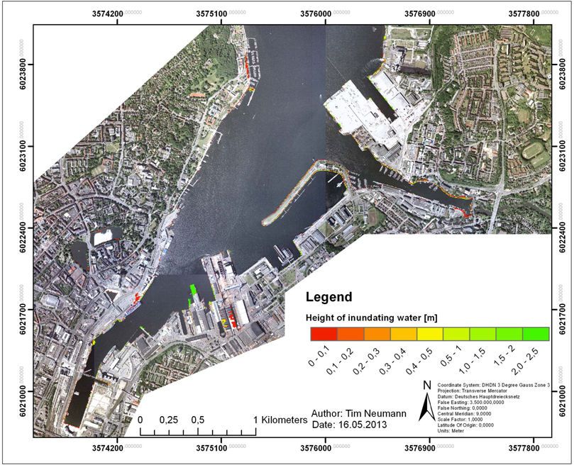
Comparing the „Bathtub Method“ with Mike 21 HD Flow Model for Modelling Storm Surge Inundation
Figures
Figure 1: Kiel Inner Fjord – Study Area……………………………………………………………14
Figure 2: Differences between geoid and ellipsoid………………………………………………17
Figure 3: Example of an output “xyz-file” from a DEM measurement………………………….18
Figure 4: Generating the DEM……………………………………………………………………..18
Figure 5: Variogramm of the study area…………………………………………………………..20
Figure 6: Variogramm of the results from the trend for elevation………………………………21
Figure 7: Upper surface represents the kriging, lower surface shows nearest neighbour
calculation………………………………………………………………………………..21
Figure 8: Results of Cooper et al. from their inundation investigation of Kahului Harbour
Area, Hawai………………………………………………………………………………24
Figure 9: Sketch of the control volume for the mass conservation...…………………………..26
Figure 10: Time centering between x and y sweep………………………………………………28
Figure 11: Order of calculating sweeps……………………………………………………………28
Figure 12: Dots represent the water level gauges within the study area………………………29
Figure 13: Validation of MIKE21 comparing to in-situ measurement at Geomar……………..29
Figure 14: “Quasi calibration” of MIKE21 calculating Daisy proper…………………………….32
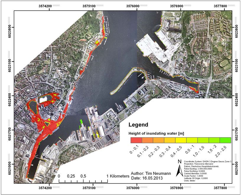
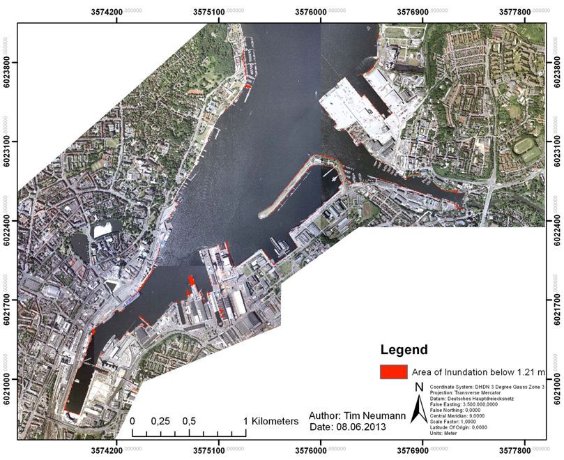
Figure 15: Inundation of Daisy without SLR, max. water level (MWL): 1.21m………………..34
Figure 16: Inundation of Daisy + SLR 0.33m, (MWL): 1.54m…………………………………..35
Figure 17: Inundation of Daisy + SLR 1.25m, (MWL): 2.46m…………………………………. 35
Figure 18: MIKE21simulation of Daisy; SLR: 0.00m Manning coefficient 32, MWL: 1.21m…36
Figure 19: MIKE21simulation of Daisy; SLR: 0.33m Manning coefficient 17, MWL: 1.54m…37
Tables
Table 1: Land-cover classes and relating Manning parameters………………………………. 16
Table 2: Workflow…………………………………………………………………………………... 22
Table 3: Statistics of the model quality…………………………………………………………… 31
Table 4: Numerical results of surface analysis in GIS of three different scenarios in ArcGIS
and MIKE21 with additional simulation runs on different resistance values……….. 38
Table 5: Relative overestimation of BTM in respect to MIKE21 for 2-D areas………………. 38
Table 6: Relative overestimation of BTM in respect to MIKE21 for 3-D areas………………. 39
6
Comparing the „Bathtub Method“ with Mike 21 HD Flow Model for Modelling Storm Surge Inundation

                                             7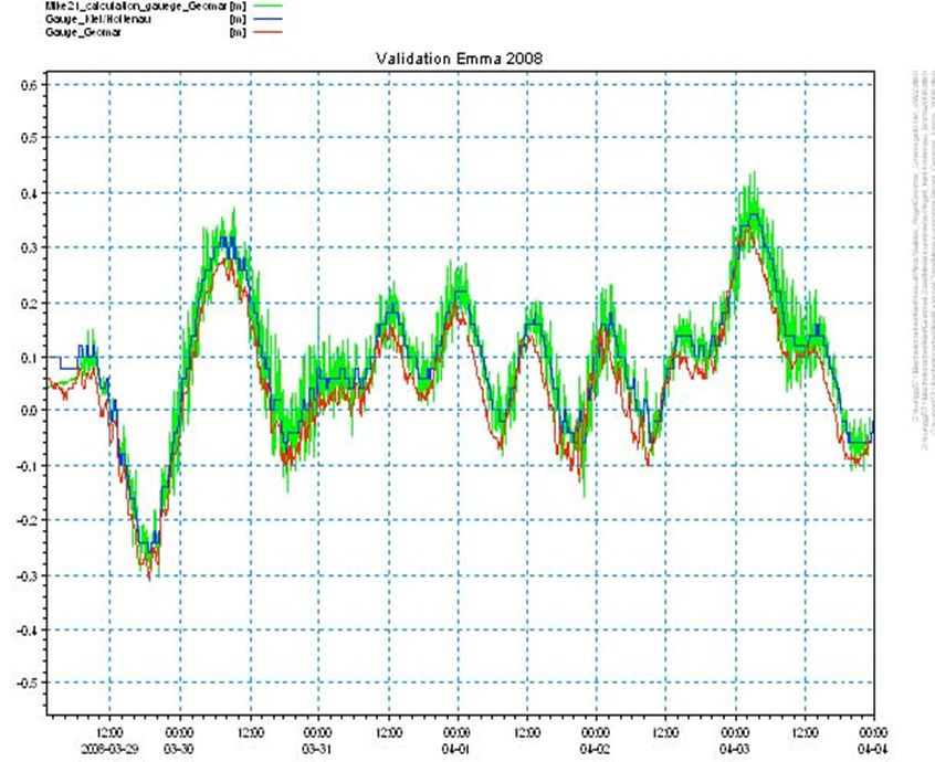
Comparing the „Bathtub Method“ with Mike 21 HD Flow Model for Modelling Storm Surge Inundation

Abstract
Meteorological measurements in the past showed that the climate is changing rapidly over
the last decades with an increasing tendency. It is expected that this trend will further
increase in the future. Therefor there is a growing interest in understanding corresponding
effects. One of the most challenging effects are floods. Due to the willing to evolve a sounder
understanding of processes take place during an inundation event, there is an immense
development of methods to analyse. This work deal with a comparison between the common
"bathtub method" and a state-of-the-art hydrodynamic model, called MIKE21 HD Flow Model,
for modelling storm surges. The aim of this study is to work out the differences between both
approaches and to find out how probable differences look like. There is the question if the
"bathtub method" represents flooding adequate or, if the consideration of physics by
hydrodynamic models makes a major difference and displays maybe the "real" risk of
inundations. This work tries to underline the differences between those two approaches,
where the strengths and weaknesses are and what influence those differences have for an
inundation analysis. The investigation was made on a digital elevation model for the study
area of Kiel, the capital city of the state Schleswig-Holstein in Germany. It is a midsize city of
242.041 inhabitants in the south-west of the Baltic Sea. The two approaches were made on
data for a small storm surge on the basis of water-level-change and wind-regime data from
2010. The major aspect of investigation was the inundation extend under applying the
different approaches. Water-level changes were implemented by developing different
scenarios and additionally using time series from a surge for simulations. Further it was
examined what influence surface resistance could have for the study area and how this
influences the outcome of the two approaches as well as how inundation changes by taking
physical behaviour of water-surface interaction into account. The results showed a difference
between both approaches of average 11.25 % for a 2-D and 6.89 % for a 3-D surface
analysis, where the "bathtub method" overestimates the hydrodynamic modelling (HDm).
Further the outcome shows interesting behaviours when looking on different sea level rise
scenarios what can be elucidated by changing resistances due to changing friction.
Concluding the outcomes of the work, they show a distinct difference between both
approaches. Taking the HDm as "real", the "bathtub method" overestimates the area of
inundation for a storm surge. But it has to be differentiated by different scenarios. Generally a
shallower inundation seems to be more influenced by forces like friction than an event of
higher water ¬levels. By arguing so, it should always be considered to use HDMs, at least to
get a comparable result for an analysis. The outcome of this work can be seen as a hint for
inundation analysis and how to grade analysis of those two approaches.
To make a more reasonable statement about the error of the approaches further effort
should be done in future, to repeat this work on different case-studies.

                                                8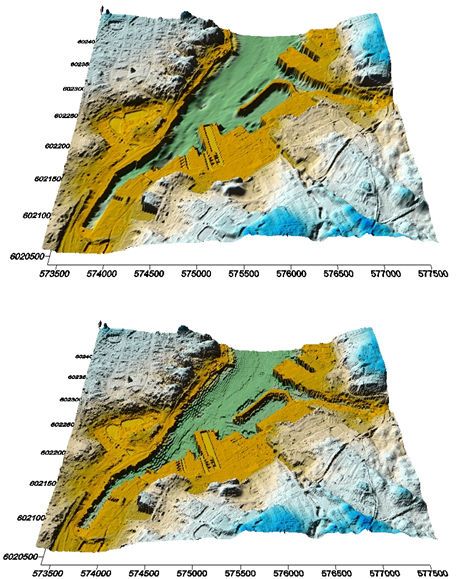
Comparing the „Bathtub Method“ with Mike 21 HD Flow Model for Modelling Storm Surge Inundation

1        Introduction
Since climate is changing rapidly the fear of natural hazards and damages increases. The
most likely consequences to global warming are accelerated Sea Level Rise (SLR) due to
thermal expansion and melting of ice as well as a change in meteorological regimes which
can produce storm surges. The most threatening impacts are floods. “In 2011, floods were
reported to be the third most common disaster, after earthquake and tsunami, with 5202
deaths, and affecting millions of people“ (Balica et al. 2013, p. 84). Also areas, which are
apparently not at high risk, are threatened. Even Europe, which has a high adaptive capacity
and a well-developed scientific base, will have to manage conditions previous not
experienced and to cope with those problems on different ways (Nicholls & Klein 2005, p.
200). “One third of the European Union population is estimated to live within 50km of the
coast“ (Nicholls & Klein 2005, p. 200; Nicholls & Klein 2005, p. 209). Comparing to other high
threatening parts of the World, a high necessity to expand sea-level impact assessment is
discernible as coastal regions become more vulnerable by changing boundary conditions
(Poulter & Halpin 2005, p. 167). Due to this demand of information it should be the aim to
apply the most reasonable approach to model and gain optimal results in terms of
preciseness and accuracy to display inundation risk. To get this information environmental
modelling is the common strategy to generate knowledge of future risks.
Models are generally a simplified representation of reality. Like a sculptor forms his physical
model with a range of techniques and tools out of clay, a scientist does the same in
mathematical manner with help of equations, based for example on a computer software.
The problem on modelling is to have a sound understanding of what is going to be inspected.
The highest task is, to observe the nature and to decide which aspects are important for
further investigations. By this a model always shows just those components which are seen
to be essential for the process. Thereby a model takes always the modellers signature. This
can lead to a not completely objective perspective of the system (Wainwright & Mulligan
2004, p. 8). However, the biggest advantage on environmental modelling is a numerical
precise hypothesis which than can be quantified and evaluated, what allows observations to
be explained and future predictions to be made (Smith 2007, p. 4-7). In general,
environmental modelling has the potential to:
1. quantify expected results
    •    recent weather trends (do we expect sufficient rainfall over the summer)
2. compare the effects of two alternative theories
    •    does an inundation reaches further inland when boundary conditions do have a
         stronger emphasis on wind conditions than on SLR
3. describe the effects of complex factors such as random variations in input
    •    how do uncertainties in C02 trends affect predictions of future climate change
4. explain how the underlying processes contribute to the observed results
    •    how changes in the quantity of one parameter can change the physical behaviour
5. extrapolate results to other situations
    •    what would the inundation look like, if there would be an additional meter of wave
         height

                                                 9
Comparing the „Bathtub Method“ with Mike 21 HD Flow Model for Modelling Storm Surge Inundation

6. predict future events
   •   if SLR will be 1,9 meter above MSL by 2100 the inundation will look like...
7. translate science into a form that can be easily used by non-experts
   •   weather forecast allows us all to make use of complex meteorological science
The use of environmental modelling is based on the context concerning climate change
(Wainwright & Mulligan 2004, p. 1). They can develop and improve our understanding for
environmental processes. Although most processes are not observable, their affects and
effects are measurable and can be used for modelling. Therefor it is often difficult to
distinguish between the environmental process and the outcome which is modelled incorrect.
But it does provide at least a base for investigations (Wainwright & Mulligan 2004, p. 1).
Because there is such a huge margin of parameters in environmental modelling, parsimony
is one of the highest principles. In a modelling context, parsimony means a high as possible
explanation and simplicity while the complexity and amount of parameters should be as less
as possible. “It is a particularly important principle in modelling since our ability to model
complexity is much greater than our ability to provide the data to parameterise, calibrate and
validate those same models. Scientific explanations must be both relevant and testable. Non-
validated models are no better than untested hypotheses“ (Wainwright & Mulligan 2004, p.8).
To combat the problems of flooding, inundation modelling is done in different ways. The key
task of all inundation assessments is to predict future water levels and inundation extent that
result from particular trigging combinations such from meteorological and tidal conditions
(Bates 2005, p. 794). Inundation modelling, which addresses the above mentioned problem
of flood risks, has the aim to predict e.g. storm-induced coastal flooding on an accurate
manner (Cheung et al. 2003, p. 1354). Methods combining geographical information systems
(GIS), remotely sensed data and numerical models have been developed to deal with these
difficulties and to understand flood risk (Wadey et al. 2013, p. 2). In the context of inundation
modelling immense problems are uncertainties like the upcoming SLR. The
Intergovernmental Panel on Climate Change (IPCC) estimates in its six “SpecialReport on
EmissionScenarios“ marker scenarios (SRES) an upcoming SLR of 0.37m for the lowest
estimation, named “B1“, to 0.58m, called “A1FI“ by 2100. This SLR will be based on thermal
expansion and melting of ice (IPCC 2007, p. 323). However, to get an idea about this, the
example of ice-sheet melting rates can demonstrate uncertainties. If these discharge rates
are linear until 2100 there will be an additional SLR of 0.05m to 0.11m, which has to be taken
into account for “A1FI“. Anyway, in sum this would lead up to 0.69m SLR (sum of the general
SLR from A1FI of 0.58m plus ice melting of 0.11m), which is 86.5% more than the lowest
assessment.
These numbers are of interest for long term investigations but don't have a huge effect for
storm surge modelling nowadays, because "the annual SLR increment is about an order of
magnitude smaller than the vertical error of most elevation datasets" (Poulter & Halpin 2005,
p. 168). Furthermore the effect of changing meteorological-regimes due to climate change
are classified and expected to be much more threatening in terms of temporal extreme water
levels than SLR. Even this is strongly discussed and under worse assessable uncertainties
(Graham 2008, pp. 197-198).
A more significant problem is the resolution of the digital elevation models (DEM), which are
the basic data of environmental modelling whereas those data are the "playground" the
modelling is based on. In general a DEM gets interpolated to a homogenous grid of a defined
resolution e.g. 10x10m. Once this interpolation is processed the DEM may contains

                                               10
Comparing the „Bathtub Method“ with Mike 21 HD Flow Model for Modelling Storm Surge Inundation
significant topographic uncertainties in the surface (Marks & Bates 2000, p. 2110). This can
results in a worse vertical accuracy. "Consequently, the model is of a much higher resolution
than the basic topographic data set and, with rapid improvements in computational power,
this situation is likely to get worse" (Marks & Bates 2000, p. 2110).
It is obvious that uncertainties do have an immense influence on what areas are modelled to
be under inundation stress. Therefore Hulme et al. mentioned in the IPCC Assessment
Report 4 (AR4), chapter 6 (Coastal systems and low-lying areas) that coastal impact
scenarios should take additional 50% of the amount of mean SLR into account, plus local
factors to the initial sea surface prediction to compensate uncertainties. Those factors could
be local uplift or subsidence of the land (IPCC 2007, p. 324; Poulter & Halpin 2005, p. 170).
The reason including these factors is to give coastal managers a higher potential sea level
for their planning to gain extra safety in their undertakings of coastal management issues
(Nicholls & Klein 2005, p. 211-214).
Two often applied approaches in inundation modelling are the "Bathtub Method" (BTM) and
hydrodynamic modelling (HDm), which are going to be the approaches applied in this study.
The main idea behind the BTM is, an area which lies under a certain height, gets flooded like
a bathtub. An example is the flood warning system of the city Kiel (http://ims.kiel.de/extern/
kielmaps/?view=katschu&) (Landeshauptstadt Kiel 2008). It gives inundated areas for a
particular corresponding height. But this Kiel application is a web based GIS and it is strongly
limited to the user. It is just a geographical presentation of different elevation levels. There
are no possibilities for the user to produce own results. It just shows pre-produced results.
Rodriguez (2010) presents in his work "Mexican Gulf of Mexico Regional Introduction and
Sea Level Rise Analysis of the Carmen Island, Campeche, Mexico Region" a way of how to
work with a DEM and how to get information about inundations. A solution to determine
inundation areas is to reclassify a DEM to the scenarios height, like Klein and Nicholls (1998)
show in the example “Use of satellite data and GIS in a coastal impact assessment for
Poland”. Rodriguez technique is much more detailed and gives more output to analyse, thus
he also undertakes a 3-D analysis to generate numerical precise statements. He formulated
his method to determine coastal effects for the region of Carmen Island in the Mexican Gulf
of Mexico. His considerations were based on a, to global climate change associated, SLR
estimation of 60cm by 2100. The coastal effects were investigated on the SRTM DEM of a
resolution of 90x90m.
A result of his research was a two coloured map, showing areas which are equal or less then
60cm of height in one colour and the rest in another one. This new produced raster was
superimposed on the original DEM and made transparent so the areas of inundation were
apparent.
For final analysis of landmass loss, the above mentioned 3D-analysis was processed on the
entire DEM to calculate the statistics. The results of the statistics were presented in tables
(Rodriguez 2010, p. 1-18). The advantage of this approach is the dimensional analysis
instead of just graphical interpretation like in the example of Kiel. Summarised a BTM
inundation analysis is a four part framework:
1. First task: collect and generate data:
• with special focus on DEM
2. Second step: pre-processing of the DEM, its parts and task are:
• geo-referencing (to make sure analysis will be in the right spatial frame)
11Comparing the „Bathtub Method“ with Mike 21 HD Flow Model for Modelling Storm Surge Inundation
• if possible validating vertical values
3. Step three: prepare and analyse the DEM:
• applying the Scenario (to get in detail selection for area of interest)
• selecting area of interest
• reclassification
4. The fourth step is analysing:
• processing of maps, graphical analysis of inundation
• spatial calculations of inundation
The approach of HDm is the second tool for developing coastal flood management policy
which will be discussed here. The model, used in this study is the MIKE21 HD Flow Model by
DHI (Danish Hydraulic Institute). In the case of assessing coastal hazards, 2-Dimensional
horizontal solutions of the shallow water equations (SWE) are currently the state-of-the-art
tools. In shallow seas, such as coastal bays and estuaries are, models which are based on
those equations provide simulations of water levels in good realistic manner (Bates 2005, p.
794). The interactions between the medium and the earth surface are elementary
components in the process of inundation. Due to the movement of water particles forces
arise like currents which can emerge by the influence of wind. Wind also could lead to a
changing wave regime. Different wave-wind-regimes obvious lead to different risk potentials.
These factors are so called hydrodynamics and are considered in HDm.
However, like mentioned above, the resolution of the DEM is the most crucial point to gain
acceptable results. Whereby the resolution should be more detailed the smaller the scale of
the study area is. For example, in case of a damage appraisal on local scale, the
computational grid should resolve 50m or less. For an observation on regional scale Bates et
al. (2005) suggest a resolution of 200 - 50m. Anyhow it is difficult to distinguish between the
process or the outcome which is simulated in a reasonable manner, to determine a sound
understanding of the risk and risk providing parameters it has to be simulated a set of runs.
Even though, the assumption of deterministic inundation modelling is highly questionable due
to parameterisation and simplification in solving equations (Bates 2005, p. 794). To gain
accuracy and significance there is the demand to evaluate and compare different sets of
input-parameter which are maybe equal likely to determine computational demands. But by
running different sets there is a growing workload on computing resources. Regarding this,
the development of hydrodynamic models (HDM) gets improved in the direction to evolve
systems which are capable to capture all essential physics to simulate substantial
mechanisms of flooding, but at significant lower computational cost (Bates 2005, p. 794;
Wainwright 2004, p. 8).
Anyhow like the BTM, a HDM is also just an assumption of reality. The SWE are an
assumption which is derived from reality.
This work will compare this both approaches. The aim is to figure out, how the main
differences, taken physics into account or not, are influencing the results of inundation
simulations on the study area of Kiel. Three different scenarios were simulated, one is a
small storm surge in the Baltic Sea, one additional with a weak SLR and one with additional
a maximum SLR, to see different percentage variation of inundation comparing the HDm and
BTM regarding the physics of the HDM. It will be the aim to show different influences to the
inundation by different water levels with emphasis on changing determining factors which
effect the inundation extend.
12Comparing the „Bathtub Method“ with Mike 21 HD Flow Model for Modelling Storm Surge Inundation
2 Methodology
2.1 Study area
This work is based on the study area of Kiel, the capital of the state Schleswig-Holstein in
Germany. More precise the investigations were done on the inner Fjord of the city (Fig. 1).
The data for the terrestrial DEM for the investigations are based on the amtliche
topographische-kartographische Informationssystem (authoritative topographical-
cartographical information system, ATKIS) catalogue which is a database for digital
landscape models. It was generated by the State Surveying Authority of Schleswig-Holstein.
The original resolution is 1x1m and displays the elevation of the land (Amtliches
Topographisch-Kartographisches Informationssystem 2008). This basic data was provided
by the Geographical Institute of the University of Kiel. The second part of the basic data for
the DEM was the bathymetry of the Kiel Fjord. The measurement was carried out by the
Bundesamt für Seeschifffahrt und Hydrographie (BSH; National Authority for maritime
navigation and hydrography). It represents the depth of the water instead of the heights and
has a general resolution of 30x30m. This data where provided directly by the BSH.
Generally Kiel lies at the south-west of the Baltic Sea. The region is certainly shaped in the
Weichselian glacial period. The narrow and deep shape of the Fjord is related to erosion by
glaciers and melt-waters. In the last 130 years anthropogenic modifications took place and
influenced the shape essentially (Kögler & Ulrich 1985, pp. 1-3). The recent waterfront shows
different highly frequented utilisations like harbours, tourism, shipyards, residences and
catering. Nowadays the waterfront is characterised by long parts of sea walls and relatively
high lying. Inundation events are relatively rare because of the elevation. For an inundation
event particular trigging circumstances have to occur. For example northerly to easterly
winds have to prevail in a strong manner to negligible tides, an inundation usually is a wind
driven phenomenon. The most known threatening event was the storm surge from 1872, with
a water level of 3.40m above MSL (Geckeler, Ynr).
13Comparing the „Bathtub Method“ with Mike 21 HD Flow Model for Modelling Storm Surge Inundation
Figure 1: Kiel Inner Fjord - Study-Area; Source: Top25, Landesvermessungsamt Schleswig-
Holstein
2.2 Inundation scenario
The scenarios for the investigations were derived from an event of a relative high probability
and, to create a theoretically future risk event, additionally SLR was taken into account. The
deliberation was to choose an event which had on the one hand a high water level, but on
the other hand also a high probability of occurrence. To figure out inundation areas at this
study area, an event of relative high water levels had to be simulated to get inundated areas
because the coastline of Kiel has relatively high altitude. A storm called Daisy from 2010 was
chosen as basic hydro-meteorological event. It represents a common storm event for the
area of the south western Baltic and had average values in respect of a storm in water level
14Comparing the „Bathtub Method“ with Mike 21 HD Flow Model for Modelling Storm Surge Inundation
heights and wind velocities. Water levels up to 1.5m were measured as maximum in the
Baltic and the wind-regime was a north easterly of 7-8 Beaufort up to a violent storm (BSH
2013a, p. 1). The maximum difference to MSL for the gauge Kiel-Holtenau was 1.21m at
6:46 in the morning of the 10‘Th of January regarding the measurements. A small storm
surge at the German Baltic coast is by definition of a height between 1-1.25m (BSH 2013b).
This kind of event can be expected during the strong winter and spring storms every three to
four years or even oftener. Defining a storm surge, it describes the time range of high water
levels, but not only the maximum water level (MWL) itself. However the MWL is the indicating
factor to classify the surge (Schumacher 2003, pp. 83-90; Schumacher 2003, p. 98). Due to
the fact that most scenarios focus to the year 2100, the focus felt on predictions for this time.
Down scaled models were generated on basis of emission scenarios and produced for the
Baltic regionally different mean sea levels. Those models indicated the risk will be highest in
future climate for the eastern and southern parts of the Baltic. A probable SLR of 33 -125 cm
by 2100 which is in average 75 cm (Graham 2008, pp. 197-198) is predicted. There is no
overall agreement and obvious uncertainties, but this information was taken for the scenarios
which should be the base for the MIKE21 and BTM investigations. Furthermore it was
mentioned that extreme sea levels will increase significant more than the mean sea level due
to changing wind regimes. But this will not be taken into account at this place, because of the
increasing uncertainty and the increasing demand to validate the model further. Due to this
information different scenarios were considered:
(a) Daisy as a stand-alone event with a maximum water level of 1.21m
(b) 0.33m as lowest SLR for the Baltic in addition to Daisy
(c) 1.25m as highest SLR for the Baltic in addition to Daisy
Because the main advantage of Hdm in respect to BTM is the physics, the advisement was
done to run the scenarios with different surface resistances. As primary information Tab. 1
was used, where the different resistance coefficients were taken from (Kaiser 2011, p. 2525).
The decision fell on a Manning coefficient M of 32 as default set-up in MIKE21. Further there
were runs done with a Manning M of 17 as middle density urban area and 12.5 for high
density urban area. Due to the limited information and time a further land cover classification
was not carried out, so these values got assumed for the whole area. An additional
improvement would be to classify for example each building and to generate, by using
remote sensing, differentiated roughness maps. But this would exceed this work at the
moment.
15Comparing the „Bathtub Method“ with Mike 21 HD Flow Model for Modelling Storm Surge Inundation
Table 1: Land-cover classes and relating Manning parameters; Source: Kaiser (2011), p.
2525
2.3 Digital elevation model
The main important data for this kind of environmental, spatial analysis is the "Digital
Elevation Model" (DEM). Both approaches mentioned in the introduction are limited by the
spatial resolution of the DEM (Van de Sand et al. 2012, p. 569). A DEM is a digital,
quantitative representation of the earth‘s surface. It includes and provides basic information
about the terrain. Parameters like slope, drainage area and topographic index are important
for every kind of environmental modelling and assessment. For example, they determine how
much water discharge a river has, conditioned by the slope and drainage area. Different
techniques such as photogrammetry, interferometry or airborne laser scanning are applied to
generate DEMs (Mukherjee 2013, p. 205).
The limitations of spatial approaches using a DEM are caused by different resolutions of the
generating techniques. There are public available DEMs like Aster GDEM (Advanced
Space¬borne Thermal Emission and Reflection Radiometer) or SRTM DEM (Shuttle Radar
Topography Mission). The Aster has a resolution of 30x30m; SRTM has 90x90m (Van de
Sand et al. 2012, p. 570). In comparison LIDAR (Light Detection And Ranging), which is the
airborne laser scanning technique, can resolve up to a nominal point density of 2 points/m². It
is obvious that analysis with data of higher resolution lead to more extensive results. But also
a higher resolution causes a higher amount of data, which affects a higher demand of
16Comparing the „Bathtub Method“ with Mike 21 HD Flow Model for Modelling Storm Surge Inundation
computer memory capacity. A higher data density also requires a higher amount of
computing capacities to get results in an acceptable amount of time.
Following Wainwright and Mulligan, "something is complex if it contains a great deal of
information that has a high utility, while something that contains a lot useless or meaningless
information is simply complicated“ (Wainwright & Mulligan 2004, p. 2). It should be the aim to
make problems complex rather than complicated. The optimal model is the one that contains
sufficient information, but not more. “Any approaches, whether it is a qualitative description
or a numerical simulation, is the try to achieve this aim“ (Wainwright & Mulligan 2004, p. 2).
Therefor the resolution of a DEM should be functional in respect to the question of
investigation.
However, those data measured are set into a 3-dimensional coordinate system. Due to
support of global positioning systems (GPS) every measured value of altitude, which are the
z-values, gets coordinates in “x“ and “y“ direction. In result it is a “.xyz“ file which gets further
processed to a DEM. What kind of format this x and y values are transformed to, depends on
the definition of the reference datum and coordinate-system. Due to the fact that most of the
measurements are made supported by GPS the common datum is the World Geodetic
System 1984 (WGS84) which the datum GPS is based on. The elevation of a point of the
local earth surface in respect to mean sea level (MSL) can vary to the elevation computed by
GPS. The GPS coordinates are computed on basis of the WGS84 ellipsoid. The earth
instead is the geoid, what can result in differences in elevation between geoid and ellipsoid.
“The geoid surface is an equipotential or constant geo-potential surface which corresponds
to mean sea level. The geoid height/geoid undulation (N) is the difference in height between
geoid and ellipsoid at a point“ (Mukherjee 2013, p. 206). However it can be derived that: h =
H + N where is: h = represented ellipsoid height, H = height above geoid surface, N = geoid
height, see Fig. 2 (Mukherjee 2013, p. 206). This means GPS could overestimate the real
height depending on localities.
The two following examples show, how these data look like when taken and written by the
measuring systems and how they look after processing. In Fig. 3 every line represents one
coordinate point. The first column is the x, the second column the y and the third column the
height, the z coordinate. If all points are computed the result can look like Fig. 4. Depending
on the resolution (point density of the measurements) the DEM gain or loses extent. The
example in Fig. 4 represents a DEM of Kiel. Like mentioned above the generation of this
basic data is an essential part of getting information about inundation.
Figure 2: Differences between geoid and ellipsoid; Source: Mukherjee (2013), p. 206
17Comparing the „Bathtub Method“ with Mike 21 HD Flow Model for Modelling Storm Surge Inundation
3570000 6019040 11.03
3570005 6019040 10.95
3570010 6019040 10.82
3570015 6019040 10.85
3570020 6019040 10.88
3570025 6019040 10.89
3570030 6019040 10.90
3570035 6019040 10.92
3570040 6019040 10.94
Figure 3: Example of an output “xyz-file“ from a DEM measurement
Figure 4: Generating the DEM : Example of a “xyz“ file after processing, resolution 10X10m
2.4 Preprocessing
The land and water area data set have to be combined to get one homogenous DEM for the
land side as well as for the water area. The DEM data were airborne generated,
measurements of the water area were taken by sonar. The ATKIS DEM had to be “cleaned“
from values of the water area with the effect of having no more information of the DEM in the
Fjord. Otherwise these areas would provide errors when interpolating. This was done within
ArcGIS by creating a polygon of the coastline and deleting everything within it. The corrected
DEM of Kiel became the basis for the BTM investigation later on.
Both datasets are ASCII file which further became processed by the editor software TextPad.
It has the ability to work in columns and rows within ASCII files, so both datasets were
brought together, adjusted and formatted to a conform shape. Before processing further it
had to be considered which area of the Fjord was of interest, for what a list of three decision
guidance points were constructed:
• The area should be as small as it was practical for an inundation simulation; to
minimise computation demands
18Comparing the „Bathtub Method“ with Mike 21 HD Flow Model for Modelling Storm Surge Inundation
• The area should show a distinctly inundation in the web-GIS of the city Kiel to
increase the probability of inundation while Hdm (because of expectation of less
inundation in modelling approach due to physical interactions)
• The area should be of a certain economic interest (for eventually further
investigations like vulnerability assessment)
The coordinates of the Inner Kiel Fjord are:
Lower left corner: 3573400 x-direct. / 6020400 y-direct.
Lower right corner: 3577500 x-direct. / 6020400 y-direct
Upper left corner: 3573400 x-direct. / 6024040 y-direct
Upper right corner: 3577500 x-direct. / 6024040 y-direct
After pre-processing a complete ASCII file was created as a .xyz file for the area of interest
(AOI). The further processing went on with interpolating the joined data due to the fact that
both basic data had different resolutions. To get homogenous resolved DEM software for
contouring and 3D surface mapping, called Surfer by Golden Software was used. Using this
software it was enabled to generate a controlled grid with acknowledge of the background
geo-statistics. Within Surfer kriging was described as a flexible method to generate good
griding results (Golden Software 2002, p. 117). In Surfer kriging can be used as interpolator
which “incorporates anisotropy and underlying trends in an efficient and natural manner“
(Golden Software 2002, p. 117). Anisotropy describes the equality of a parameter in a
direction compared to another one. To give an example, imagine a shoreline where the
probability of equal sediment parallel to the shoreline is more likely as perpendicular to it
(Golden Software 2002, pp. 108-109). Because there was anisotropy due to the two different
densities in the datasets it was decided to use kriging. To get an overview about the spatial
distribution, the spatial dependence of points to each other, as well to provide the needed
information for interpolating the data by the kriging method, a variogram was produced (Fig.
5). Variogram are used to investigate how grid-points do relate to each other in the manner
of spatial dependence. It shows how far a certain point has to be away from a central point,
on which the measurement is based on, to be un-associated to it. In Fig. 5 the experimental
variogram is displayed by the dots. A fitted model is shown as solid blue line, which is the
function the kriging was based on for an interpolation. Beside visible in Fig. 6 is the
plateauing of a variogram. The beginning of the plateauing is the distance where points are
no longer associated to each other. It is the so called “range“.
As mentioned above, that information are needed to ensure a reasonable interpolation when
the kriging method is used (Harris, R. & Jarvis, C. 2011, p. 209).
The key behind this concept is to calculate the variance as a function of the distance away
from a central point. This is computed for each point to every other one in the data set. The
calculated variance values are assigned in so called “lags“ which are sections of distances
from zero to the maximum measurement of distance. The maximum measurement of
distance is equal to the maximum search radius from a central point, to points which are
gone to be compared in terms of variance. The measured variance in dependency to the
distance can be plotted as an experimental variogram, shown in Fig. 5 (black line with dots).
19Comparing the „Bathtub Method“ with Mike 21 HD Flow Model for Modelling Storm Surge Inundation
Figure 5: Variogram of the Study area produced with Surfer
Further there are general rules of thumbs for the construction of a variogram. The first one is
that at least 50-100 points are needed to generate a variogram, this is case depended due to
the variation in the amount of data points in each lag. The data set for the variogram of the
study area has an absolute number of 124280 points. The second one is the maximum lag
distance should be less than half the wide of the study area (Harris, R. & Jarvis, C. 2011, p.
210-211). In this study the AOI is 4100 meter wide. Surfer uses this information and
produces a max lag distance (MLD) by default which is less the half wide (shown in Fig. 5;
half wide 2050, Surfer produced MLD 1800). The most conspicuous is that there is no
plateau. This means every point is associated with each other point within the maximum
distance of searching. Another point to recognise is the curve itself. Due to the fact there is
no plateau, the curve ascends continuous. This is caused of the relative high point density in
the DEM as therefor a high dependency between the points. It is likely that the variations of
the experimental variogram are little because of the different point densities of the
topography and bathymetry. To get the variogram function (blue line in Fig. 5) which is used
further as the function for interpolating, Surfer includes a range of so called models to
describe the experimental variogram. The best fitting should be used to result in a
reasonable function for the interpolation. Due to the fact the curve is nearly linear, the linear
model was chosen. By the option AutoFit within Surfer the linear model got a slope of 0.059,
anisotropy of 2, and an anisotropy-angle of 40.59, which is also caused by the lower point
density of the bathymetry in the Fjord. Due to the acceptable fitting of the variogram model,
the resulting grid after the kriging interpolation was considered to be reasonable and was
used for the further modelling investigations. However, also the nearest neighbour
interpolation was used to produce a surface, to compare the results of the kriging and the
nearest neighbour interpolation (shown in Fig. 7). By comparing the different results visually,
the nearest neighbour surface shows a rougher structure than the kriging result, especially in
the water area. Those unrealistic irregularities strengthen the relevance of the kriging grid.
The pre-processing was finished at this point.
20Comparing the „Bathtub Method“ with Mike 21 HD Flow Model for Modelling Storm Surge Inundation
Figure 6: Variogram of the residuals from the trend for elevation; Source: Oliver, M.A. & A.L.
Kharyat, (1999)
Figure 7: Upper surface represents the kriging, lower surface shows nearest neighbour
calculation
The following Tab. 2 gives an overview of the working steps in general. It represents the
different steps which had to be processed to generate inundation maps of the three
scenarios for the study area and to calculate the inundation statistics.
21Comparing the „Bathtub Method“ with Mike 21 HD Flow Model for Modelling Storm Surge Inundation
Table 2: Workflow
Working step Software tool Needed Data
1. Clean original DEM from water values ArcGIS 10.0 • ATKIS DEM 10x10m
• Coastline Kiel
2. Merge DEM and bathymetry data, bring it to TextPad • Corresponding ASCII files
uniform shape
3. Generate Variogram Surfer 8 • Merged ASCII file
4. Interpolate ASCII file and generate grid Surfer 8 • Merged ASCII file
• calculated variogram
5. Validating MIKE21 MIKE21 Time series of gauge:
• Kiel/Holtenau
• Geomar
Time series Wind:
• Lighthouse/Kiel
• Generated grid
6. Setting up proper SLR scenarios and MIKE21 Time series of gauge:
controlling a satisfying implementation • Kiel/Holtenau
• Literature
7. Generate BTM inundation maps (see 3.4 ArcGIS 10.0 • Generated grid
applying the two approaches) • Shape file of the Fjord
• Scenarios
8. Run simulations on different scenarios (see MIKE21 Time series of gauge:
scenarios in 3.3 Inundation Scenarios ) • Kiel/Holtenau
• Generated grid
• Land-cover roughness classification values
• Scenarios
9. Surface analysis ArcGIS 10.0 • Simulated grid files from MIKE21
• Inundation areas from BTM analysis
10. Presenting the results ArcGIS 10.0 • Surface statistics
2.5 “Bathhub” inundation approach
The following part describes how ArcGIS 10.0 was used to generate inundation maps for the
"Bathtub Method". The key behind this method was elucidated in the introduction above;
regarding this the following section will deal with the application on the study area. Like
mentioned in the section 2.4 Pre-processing the in Surfer generated grid was the base for
further investigations and the first step of applying any approach. The second step was to
convert a shape file of the water area, which was a part of the ATKIS catalogue, to a raster
with cell sizes accordingly to the cell size of the DEM. This was done by Conversion Tools -
To Raster -Polygon to Raster. The next step was to create a mask out of this new raster.
Therefor the raster had to be reclassified. This was done by Spatial Analyst Tools -Reclass -
Reclassify. The aim was to change the value of the water areas to zero and anything else to
one. So that in the fourth step the DEM values got multiplied by one and the water became
the value zero. The result was a corrected surface, where the water became zero as a base-
level and the land got its correct elevation. This step was fulfilled by the help of the tool
"Raster Calculator". Within "Raster Calculator" the statement “Con(,)“ was used to define a
condition. Basically the condition was, if the pixel value of the raster is zero, than the new
value will be zero otherwise the pixel will get the value of the DEM for this coordinate. The
fifth step was to generate the inundation area itself. Therefor again the "Reclassifying" was
used that way, the values from zero to a certain value (max water level) were classified as
zero and any value above was classified as one. The result was a two coloured map,
showing the land and the inundation. To become more accurately "Region Group" was used
in the next step to filter out the hydrological connected areas. Following Cooper et al. (2013),
they also carried out a BTM analysis for Maui, Hawaii with the aim to get a quantitatively
22Comparing the „Bathtub Method“ with Mike 21 HD Flow Model for Modelling Storm Surge Inundation
assess of the spatial distribution of inundation. Therefor they reclassified their DEM by the
given heights of the regional expected scenarios. Different to Rodriguez (2010) they
separated vulnerable areas in hydrological connected (HC) and disconnected (HDC). Areas
of HDC were mapped separately to take them into account for a “complete-as-possible“
analysis. Due to the problem of uncertainties in vertical accuracy, they calibrated and
validated the DEM on different tidal benchmarks. The reference for the tidal benchmarks was
MSL. Further they took local specification on the tide regime into account, in this case a
semidiurnal tide with a Mean Highest High Water (MHHW). In their further investigations they
produced 8 GIS vulnerability layers. They distinguished by HC plus basic DEM, HC plus
corrected DEM, HDC plus basic DEM and HDC plus corrected DEM. The results are shown
in Fig. 8. Those high resolution vulnerability maps are important to identify low lying coastal
areas. They highlight the critical need to act and improve community resiliency to climate
change.
To take this into the here applied approach, within "Region Group" some set-ups had to be
considered. So the number of neighbours had to be eight, the zone grouping should be set
as “within“ and the “Add link field“ button had to be deactivated. This was done to get pixels
which are also connected diagonal additionally to the ones which were connected on the
sides (Cooper 2013, pp. 554-555). Now having the hydrological connected areas, the raster
had to be reclassified again the way how it was done in the fifth step, again with an
inundation value of zero to the certain scenario level. In the end the results were hydro-
connected areas of an inundation for a certain scenario. At last there was the interest in
numerically precise information about the areas which were inundated. Therefor the former
generated polygon of the Fjord, which was created to correct the original DEM and to delete
the values of the water while pre-processing, was used. This polygon was further modified by
the areas of the "Kiel-pond", the "old boat-harbour" and the "Schwentine river" inflow. This
was done to subtract real water areas from the inundation areas. Without doing so, all water
areas, even the Fjord itself, would be taken into account when calculating the real size of
inundated land. In the end the displayed area of inundation had to be used as mask. By
using "Spatial Analyst Tools -Extraction -Extract by mask" the wrought inundation areas were
taken as mask to get the DEM of the corresponding area. This was necessary to get
absolute values for the numerical analysis. But it has to bear in mind, inundation is not a
stand-alone event. Moreover it is a result of different factors which can cause coastal
hazardous events. The list starts at SLR, changes in mean wave height, tidal oscillations,
changes in long shore currents, sediment transport, changes in wind direction and strength,
rainfall and due to this flooding, change in vegetation and ends in geomorphology
(Muthusankar 2013, p. 2402). Therefor the BTM can only be a way to identify exposed areas.
While using BTM for this kind of problem all physics are neglected. Inundation is not just like
the water level rises and floods a particular area. Hydrodynamics take place which are for
example flows, currents and turbulences which can be caused by flushed obstacles. Also an
important parameter during inundation is the resistance or friction. If water attains the land,
its flux behaviour changed. Depending on the structure of the surface, fluxes can be slowed
down more or less or can even block nearly completely (Kaiser 2011, p. 2522). Depending
on these parameters the area of inundation is influenced. To get those parameters within
analysis HDM were developed. Those models work on physical equations and compute
designated parameters for every grid cell. The following part provide a basic understanding
of the difference of a HDM to the BTM .
23Comparing the „Bathtub Method“ with Mike 21 HD Flow Model for Modelling Storm Surge Inundation
Figure 8: Results of Cooper et al. from their inundation investigation of Kahului Harbour Area,
Hawaii; Source: Cooper (2013), p. 558
2.6 Hydrodynamic modelling approach
In this study the HDM MIKE21 by DHI (Danish Hydraulic Institute) is applied to model an
inundation analysis for the study area of Kiel. MIKE21 is a complete software suite for
modelling 2-Dimensional free-surface flows. It is applicable in nearly every coastal area to
simulate hydrological and environmental phenomena. The hydrodynamic module is able to
perform operations on the forcing of different driving effects such as wind shear stress,
momentum dispersion, flooding and drying and wave radiation stress. It is mainly applied and
developed to calculate tidal hydraulics, wind and wave induced currents as well to simulate
storm surges and coastal flooding. MIKE21 is a universal HDM which also can be used to
model dyke breaches, tsunamis or harbour seiching (DHI 2009, p. 13-14). It simulates
unsteady 2-Dimensional flows in one layer. This means the water column is assumed as
vertical homogenous (no differentiation in stratification, e.g. of density due to salinity and
temperature). It works on the basis of the mass and momentum conservation in space and
time. The numerical applications in MIKE21 HD (hydro dynamics) run on an alternating
direction implicit technique to integrate those equations matrices, for each gridline in each
direction. To give a simplified outlook about the physics which are behind the shallow water
equations system SWE, it will be elucidated in the following section.
Following Raymond (Ynr) the SWE form a system to describe the behaviour of fluid flows.
For its plainest form to understand, there were made some requirements which are
assumed. The most important condition for the SWE to take effect is, that the horizontal
scale of flow is large compared to the depth and the water surface has a weak slope. It is
assumed that the water column has a uniform density ρ and the water layer has a thickness
h (x,y,t). The water flows, in this simplification, over a flat ground so h is equal to the
elevation of the surface. The velocity v is assumed to be independent of the depth v = v(x,y,t)
24Comparing the „Bathtub Method“ with Mike 21 HD Flow Model for Modelling Storm Surge Inundation
and nearly horizontal. Also to simplify, the bed resistance is neglected and the column is in
hydrostatic balance. Therefor the pressure is uniform over the depth. Of course there can be
a vertical flow factor due to bed elevation changes, but because this is an assumption it can
be resolved by the continuity equation after solving the SWE. In general it is a system of
three equations which are derived from the Navier-Stoke equation. The Navier-Stoke
equation is the general equation to describe fluxes and is derived from Newton’s laws,
particular the mass and momentum conservation. The SWE fundamental three parts are the:
1. hydrostatic equation
2. momentum equation
3. mass conservation
The hydrostatic equation is: dp/dz=gρ (1.1)
The pressure p over the depth z is equal to the gravity acceleration g times the density ρ.
Because the column is homogenous we can integrate over the depth as: p=gaze (1.2). The
pressure p is equal to gravitation g times density ρ times the depth z.
This is the first equation which has to be noted. Due to this averaging the problem becomes
two-dimensional and the vertical dimension is no longer of interest.
To derive the momentum equation and in this the second fundamental part it is needed to
generate the horizontal pressure gradient. The operator becomes 2-D when ∇= (∂/∂x, ∂/∂y).
From equation (1.2) we get –ρ-1 p=–g (1.3). This is the horizontal pressure gradient per
unit mass. It works as the pressure gradient in x and y direction at the surface and due to a
homogenous column for the whole body. The operator is nothing else than the split pressure
gradient in x and y direction which derives from the density. Simplified this means that the
pressure gradient derives from the height of the water column accelerated by the gravity.
Further there has the Coriolis force to be considered. The Coriolis force per unit mass is
-2Ωxν (1.4) because the vertical component is small in comparison to pressure gradient and
gravitational force it will be neglected. For neglecting this component the Coriolis force has to
be split up in horizontal and vertical components. Therefor we resolve Ω=Ωh+Ωzz into its two
parts. So the Coriolis force is -(2Ωhxν+2Ωzzxν) where the first part represents the vertical
component (h for height in vertical direction) which will be again neglected. Resulting in the
so called Coriolis parameter, which will be further used, is named ƒ=2Ωz=2ΙΩΙsinΦ where Φ
is the angle of latitude. The retained part is thus -ƒzxν combined with the pressure gradient
force the momentum equation is obtained from Newton‘s second Law as:
g (1.5)
This means that the velocity v over the time t derives from the pressure gradient force plus
horizontal Coriolis parameter. At a given time t the velocity is as high as the pressure
gradient and the Coriolis parameter enable it to be. Because the column is homogenous this
can be assumed over the depth. It is the second fundamental part of the SWE system.
The third key point is the mass conversation therefore we will use a sketch as example.
Imagine the water column in the sketch (Fig. 9) is a cuboid of the side length L. Simplified the
time rate of changing the volume is equal to the net inflow from both sides x and y.
25You can also read