Combining resistivity and frequency domain electromagnetic methods to investigate submarine groundwater discharge in the littoral zone - HESS
←
→
Page content transcription
If your browser does not render page correctly, please read the page content below
Hydrol. Earth Syst. Sci., 24, 3539–3555, 2020
https://doi.org/10.5194/hess-24-3539-2020
© Author(s) 2020. This work is distributed under
the Creative Commons Attribution 4.0 License.

Combining resistivity and frequency domain
electromagnetic methods to investigate submarine
groundwater discharge in the littoral zone
Marieke Paepen1 , Daan Hanssens2 , Philippe De Smedt2 , Kristine Walraevens1 , and Thomas Hermans1
1 Laboratoryfor Applied Geology and Hydrogeology, Department of Geology,
Ghent University, Krijgslaan 281-S8, Ghent, 9000, Belgium
2 Research Group Soil Spatial Inventory Techniques, Department of Environment,

Ghent University, Coupure links 653, Ghent, 9000, Belgium

Correspondence: Marieke Paepen (marieke.paepen@ugent.be)

Received: 10 October 2019 – Discussion started: 22 January 2020
Revised: 17 April 2020 – Accepted: 3 June 2020 – Published: 15 July 2020

Abstract. Submarine groundwater discharge (SGD) is an im-           freshwater lens below the dunes and flows underneath a thick
portant gateway for nutrients and pollutants from land to sea.      saltwater lens, present from the dunes to the lower sandy
While understanding SGD is crucial for managing nearshore           beach, which is fully observed with ERT. Freshwater out-
ecosystems and coastal freshwater reserves, studying this           flow intensity has increased since 1980, due to a decrease
discharge is complicated by its occurrence at the limit be-         of groundwater pumping in the dunes. FDEM mapping at
tween land and sea, a dynamic environment. This practical           two different times reveals discharge at the same locations,
difficulty is exacerbated by the significant spatial and tempo-     clearly displays the lateral variation of the zone of discharge,
ral variability. Therefore, to capture the magnitude of SGD,        and suggests that FSGD is stronger at the end of winter com-
a variety of techniques and measurements, applied over mul-         pared to the beginning of autumn. ERT, CRP, and FDEM are
tiple periods, is needed. Here, we combine several geophysi-        complementary tools in the investigation of SGD. They pro-
cal methods to detect zones of fresh submarine groundwater          vide a high-resolution 3D image of the saltwater and fresh-
discharge (FSGD) in the intertidal zone, upper beach, dunes,        water distribution in the phreatic coastal aquifer over a rela-
and shallow coastal area. Both terrestrial electrical-resistivity   tively large area, both off- and onshore.
tomography (ERT; roll-along) and marine continuous resis-
tivity profiling (CRP) are used from the shallow continental
shelf up to the dunes and combined with frequency domain
electromagnetic (FDEM) mapping in the intertidal zone. In           1   Introduction
particular, we apply an estimation of robust apparent elec-
trical conductivity (rECa) from FDEM data to provide reli-          The interface between land and sea is a complex envi-
able lateral and vertical discrimination of FSGD zones. The         ronment, with groundwater discharging from the land to
study area is a very dynamic environment along the North            subterranean estuary and saltwater intruding into coastal
Sea, characterized by semi-diurnal tides between 3 and 5 m.         aquifers (Duque et al., 2020). Submarine groundwater dis-
CRP is usually applied in calmer conditions, but we prove           charge (SGD) and seawater intrusion (SI) are complemen-
that such surveys are possible and provide additional infor-        tary processes, both subjected to the balance between hy-
mation to primarily land-bound ERT surveying. The 2D in-            draulic and density gradients in groundwater and seawa-
version models created from ERT and CRP data clearly in-            ter (Taniguchi et al., 2002). SGD is a combination of
dicate the presence of FSGD on the lower beach or below             fresh SGD (FSGD) and recirculated saline groundwater dis-
the low-water line. This discharge originates from a potable        charge (RSGD) (Taniguchi et al., 2002). It is driven by
                                                                    the terrestrial hydraulic gradient, water level differences at

Published by Copernicus Publications on behalf of the European Geosciences Union.
3540         M. Paepen et al.: Combining resistivity and frequency domain electromagnetic methods to investigate SGD

permeable barriers, wave set-up, tides, storm- or current-           under low-induction-number (LIN) conditions (e.g. CMD-
induced pressure gradients, convection, seasonal freshwater–         MiniExplorer, DUALEM-421S, Geonics EM34, and Geon-
seawater interface movement, bioturbation, and geothermal            ics EM31) provide apparent electrical conductivities (ECa)
heating (Taniguchi et al., 2002, 2019; Michael et al., 2005;         which are not valid in highly conductive environments (Mc-
Burnett et al., 2006). Its total flux is significant, since it oc-   Neill, 1980; Hanssens et al., 2019). This limitation is proba-
curs over large areas (Burnett et al., 2003), probably being         bly why FDEM has only rarely been applied in the intertidal
more important to the oceanic budgets of nutrients, carbon,          zone and only the ECa values were used in the interpretation
and metals than rivers (Moore, 2010).                                of these studies.
   FSGD can lead to eutrophication (e.g. Colman et al.,                 Both FDEM and TDEM methods are also available for
2004), blooms of harmful algae (e.g. Lapointe et al., 2005),         airborne surveys, allowing for the expansion of coverage
and it can result in a significant loss of freshwater. RSGD          in coastal and tidal environments; see Siemon et al. (2009)
can also have a significant impact on the dissolved nutri-           and Viezzoli et al. (2012) for some examples. These surveys
ent input when it interacts with the sediment (Rodellas et           can be combined with for instance EM (electromagnetic;
al., 2018). On the other hand, SI threatens potable water            e.g. Paine, 2003) or ERT studies on land (e.g. Viezzoli et al.,
in coastal zones. Therefore, understanding the dynamics of           2010; Goebel et al., 2019). However, airborne surveys are
saltwater and freshwater is essential for the management of          costly and often aim at large-scale structures, so they might
coastal freshwater reserves. However, the assessment of SGD          lack resolution at shallow depth, which is crucial to image
is difficult because of spatial and temporal variability in flux     local FSGD.
(e.g. Burnett and Dulaiova, 2003; Michael et al., 2005).                Next to EM, ERT is another useful geophysical method in
   Geophysical techniques can be used to delineate saltwater         mapping coastal salinity. ERT allows for imaging the sub-
and freshwater in coastal environments, facilitating the detec-      surface resistivity in 2D cross sections of 3D, after the data
tion of FSGD and SI. Electrical and electromagnetic methods          are inverted. The depth of investigation and resolution of
are particularly suited for spatial and temporal salinity delin-     ERT are respectively proportional and inversely proportional
eation in coastal environments given their sensitivity to (wa-       to the electrode spacing but also depend on the distribution
ter) electrical conductivity. Below we give an overview of the       of the subsurface resistivity and the chosen electrode array
methods used in coastal research.                                    (Dahlin and Zhou, 2004). The ERT cables and electrodes re-
   Time domain electromagnetic (TDEM) methods are                    main fixed during the measurement so that it can be used
mostly used for 1D soundings in coastal studies, for instance        above the high-tide mark (e.g. Goebel et al., 2017) and in
to measure salinity onshore (e.g. Goldman et al., 1991) or           the intertidal zone to measure for instance the tidal effect on
offshore using a floating system (e.g. Goldman et al., 2004).        groundwater exchange (e.g. Dimova et al., 2012). Time-lapse
Ground-based TDEM is time consuming and thus difficult to            ERT is popular for monitoring SI (e.g. de Franco et al., 2009;
apply for 3D mapping. Similarly, frequency domain electro-           Ogilvy et al., 2009), including cross-hole ERT to increase
magnetics (FDEM), although mostly used onshore, can be               resolution (e.g. Palacios et al., 2020).
used offshore as well, by towing a transmitter and receiver             Resistivity surveying can be extended to water bodies by
with a boat on the seafloor (Evans et al., 1999; Hoefel and          burying cables or resting them on top of the sediments (ma-
Evans, 2001) or by keeping them above the water (Kinn-               rine electrical resistivity – MER; e.g. Swarzenski et al., 2006;
ear et al., 2013). FDEM is particularly suited for fast map-         Taniguchi et al., 2007; Swarzenski and Izbicki; 2009; Hen-
ping of an area, but its depth resolution is limited and de-         derson et al., 2010). In the case of saline water, MER pro-
pends on the subsurface conductivity and the distance be-            vides a better resolution, since the conductive water layer on
tween the transmitting and receiving coils. The technique            top has less effect on the signal compared to continuous re-
has been previously used to characterize pore water salin-           sistivity profiling (CRP), where the current has to pass the
ity in a coastal wetland (Greenwood et al., 2006) and to             water layer before entering the sediment. In addition, MER
map saltwater intrusion on Long Reef Beach (Davies et al.,           allows for collecting reciprocal data to estimate the noise
2015). It has also been combined with (continuous) verti-            level. It is more time consuming but best suited for moni-
cal electrical and TDEM soundings to investigate the dis-            toring. In contrast, by using CRP, one can easily cover sev-
tribution of saltwater and freshwater on a sandy beach be-           eral kilometres per day. In order to compensate the effect of
tween Egmond aan Zee and Castricum aan Zee (Pauw, 2009),             the water layer (between the streamer and sediment) during
combined with 2D resistivity imaging to detect plumes of             the inversion process, the bathymetry and water conductivity
freshwater on a beach in northern Wales (Obikoya and Ben-            are measured at the same time. The resolution of the mea-
nell, 2012), and combined with TDEM and onshore electri-             surements depends on the electrode spacing, height of the
cal resistivity tomography (ERT) to discriminate freshwater          waves, and boat speed. Most CRP studies found in the lit-
and saltwater in the Albufeira–Ribeira de Quarteira coastal          erature were carried out in quiet environments with limited
aquifer system (Francés et al., 2015). However, when apply-          tidal and wave activity such as Biscayne Bay (Swarzenski
ing FDEM in saline environments, it is important to know             et al., 2004), Neuse River Bay (Cross et al., 2006), Florida
that ground conductivity instruments designed to operate             Bay (Swarzenski et al., 2009), Manhasset Bay and North-

Hydrol. Earth Syst. Sci., 24, 3539–3555, 2020                                         https://doi.org/10.5194/hess-24-3539-2020
M. Paepen et al.: Combining resistivity and frequency domain electromagnetic methods to investigate SGD                     3541

port Harbor (Cross et al., 2012), Great South Bay (Cross           Belgian–French border and the city of De Panne (Fig. 1). A
et al., 2013), Jobos Bay in Puerto Rico (Day-Lewis et al.,         groundwater extraction site is situated in the dunes, exploited
2006), and the fringing reef of Santiago Island in the Philip-     by Intercommunale Waterleidingsmaatschappij van Veurne-
pines (Cardenas et al., 2010; Cantarero et al., 2019). These       Ambacht (IWVA). Potable groundwater has been pumped
are sometimes combined with radon-222 (e.g. Swarzenski et          there since 1967.
al., 2004, 2009), MER (e.g. Swarzenski and Izbicki, 2009),             A low-lying polder area borders the dunes in the south.
seismics (e.g. Russoniello et al., 2013; Cross et al., 2014),      The shore in the north is tidal dominated (semi-diurnal), with
EM logs in temporary boreholes (e.g. Krantz et al., 2004), or      a tidal range of over 5 m at spring tide and approximately
salinity measurements (Cardenas et al., 2010; Cantarero et         3 m at neap tide. The beach is relatively flat with an average
al., 2019).                                                        slope of 1.1 % (Lebbe, 1981). The shore morphology, tidal
   Most of the geophysical studies identified above do not         range, and permeability of the phreatic aquifer determine the
bridge the gap between the land and marine realms. Offshore        presence of a saltwater lens under the shore; saltwater can in-
and onshore surveys are rather performed separately, espe-         filtrate on the backshore during high and spring tide and dis-
cially if conditions are difficult, e.g. strong tidal and wave     charges on the foreshore and/or seabed (Vandenbohede and
activity. Additionally, the spatial and temporal variability of    Lebbe, 2006).
FSGD make it more challenging. Onshore surveys alone are               The sandy aquifer is around 30 m thick at the shore and up
generally not sufficient to image the full extent of the FSGD      to 50 m in the dunes (due to a recent aeolian sand cover) and
zone, while offshore surveys miss the necessary connections        bounded by Late Eocene heavy marine clays of the Kortrijk
with onshore freshwater aquifers. Similarly, while FDEM            Formation, which are considered impermeable. The aquifer
surveys allow for faster mapping at a higher resolution of the     is relatively homogeneous at the Belgian–French border; the
salinity than resistivity methods, they do not bring sufficient    upper part is fine medium sand, and the lower part has more
information on the vertical distribution of salinity.              coarse and medium sands. It becomes more heterogeneous
   In this paper, we combine for the first time ERT, CRP, and      towards the east, with the local occurrence of clayey–silty
FDEM. The objective of the survey is to qualitatively map the      fine-sand lenses (e.g. Lebbe, 1978, 1999). For instance, a
lateral and vertical distribution of saltwater and freshwater      clay lens occurs between -5 and -10 mTAW (compared to
and identify the FSGD zone underneath the nearshore con-           the mean sea level at low tide in Ostend, which is the Bel-
tinental shelf, intertidal zone, upper beach, and dunes, at the    gian reference level) under the upper beach and fore dunes
De Westhoek nature reserve, Belgium. ERT and CRP pro-              in the east of the study zone (Vandenbohede et al., 2008b;
vide changes of the subsurface resistivity in 2D cross sec-        Hermans et al., 2012).
tions, while FDEM mapping with robust apparent electrical              Freshwater recharges in the dunes, forming a large fresh-
conductivity (rECa) provides additional information on lat-        water lens underneath. Part of this freshwater flows under-
eral variations in the intertidal zone between parallel cross      neath the large saltwater lens, forming a freshwater tongue,
sections. The combination of CRP during high tide and land         discharging into the North Sea around the low-water line
ERT collected at low tide ensures that FSGD and SI can be          (Vandenbohede and Lebbe, 2006). The potable water is of
accurately imaged at the limit of the low-water line. Our case     high value in the coastal region, since saltwater and brack-
study demonstrates that only a combination of the proposed         ish water are often found at shallow depth (i.e. the beach and
methods allows for fully characterizing the discharge zone in      polder area; De Breuck et al., 1974; Delsman et al., 2019).
the target area. It also shows that CRP data can directly pro-     The scarcity of freshwater in the region and the high demand
vide a reliable identification of the presence of fresher water,   of drinking supplies, especially in summer (due to coastal
even in very dynamic environments with a large tidal range,        tourism), make a comprehensive understanding of the hydro-
and that FDEM monitoring can be used to quickly assess sea-        geological system important for the sustainable management
sonal variations in FSGD in the intertidal zone.                   of the phreatic groundwater reserves.
                                                                       In the past, the migration of fresh groundwater towards
                                                                   the sea has been observed at De Westhoek by electrical well
2   Study area                                                     logging in 1980 (Lebbe, 1981, 1999) and temperature mea-
                                                                   surements (Vandenbohede and Lebbe, 2011). Several hy-
The study site is located in the most western part of the          drogeological and groundwater flow models have been de-
65 km long sandy coastline of Belgium, which is delimited          veloped showing sensitive parameters and the past, present,
by the North Sea in the north and a southwest–northeast-           and future evolution of the freshwater tongue (Lebbe, 1983,
oriented, semi-continuous dune belt in the south, which            1984, 1999; Lebbe and Walraevens, 1988; Van Camp and
varies in width. These dunes are part of a long, narrow            Walraevens, 2004; Vandenbohede and Lebbe, 2006, 2007;
dune strip that runs from Calais, France, to northern Den-         Vandenbohede et al., 2008a). However, these models are
mark. The Belgian coastal dune belt is around 2 km wide            2D cross sections and do not account for the lateral varia-
at De Westhoek – an extensive Flemish nature reserve and           tions along the coastline. The latter can be revealed by geo-
European Natura 2000 area – which is located between the           physics. In addition, conditions have changed over the years

https://doi.org/10.5194/hess-24-3539-2020                                       Hydrol. Earth Syst. Sci., 24, 3539–3555, 2020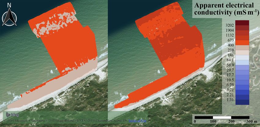
3542          M. Paepen et al.: Combining resistivity and frequency domain electromagnetic methods to investigate SGD

Figure 1. The De Westhoek study area, between the Belgian–French border and the city of De Panne. With the location of the ERT and
CRP profiles, zones of FDEM mapping, resistivity logging profiles of Lebbe (1981), and IWVA groundwater extraction site. © Microsoft
Corporation, DigitalGlobe, and CNES, 2019.

since the IWVA started a decrease of the exploitation rate at       repeated numerous times to obtain very long ERT profiles
De Westhoek in the 1990s. Nowadays, the pumping rate (ap-           while maintaining relatively homogeneous lateral sensitivity.
proximately 3.2×10⁵ m3 in 2018) is much smaller compared            It also allows for maintaining all the measuring electrodes
to the 1980s, when pumping rates were between 1.5 and               above the current tide level. Combined with a spacing of 5 m
2.2 × 10⁶ m3 yr−1 .                                                 between the electrodes, profiles of up to 625 m long were ob-
                                                                    tained. The multiple-gradient array configuration was chosen
                                                                    for its relatively fast data acquisition speed, which is critical
3     Methodology                                                   in tidal-dominated environments, and its good compromise
                                                                    between signal-to-noise ratio and resolution (e.g. Dahlin and
3.1     Electrical resistivity                                      Zhou, 2004, 2006).
3.1.1    ERT on land
                                                                    3.1.2   Marine CRP
Data acquisition
                                                                    Data acquisition
The ABEM Terrameter LS with 64 electrodes was used for
the ERT survey on land. Data acquisition took place on mul-         For the marine survey, direct-current CRP is preferred over
tiple days – 7 March (one profile 1 km east of the Belgian–         the MER mode (in which electrodes are buried or rest on the
French border, K1) and 11 October 2018 (one profile at the          seabed), since data collection is easier and faster. The use
border, K0). Measurements started during the lowest tide,           of CRP in a very dynamic environment, such as the North
allowing to measure a wide zone, with the roll-along tech-          Sea (semi-diurnal tides – tidal range between approximately
nique. Using this method, the Terrameter is placed between          3 and 5.3 m – and often relatively strong waves), is not com-
electrodes 32 and 33. After measuring, it is shifted by 16 or       mon. Measurements were only performed under relatively
32 electrodes while new electrodes are positioned at the end        calm weather conditions, with a maximum wave height of
of the profile so that the device is back in the middle of the      around 1 m and maximum wind speed of 5.5 m s−1 . CRP is
array to perform new measurements. This procedure can be            performed nearshore, both during high and low tide. The for-

Hydrol. Earth Syst. Sci., 24, 3539–3555, 2020                                        https://doi.org/10.5194/hess-24-3539-2020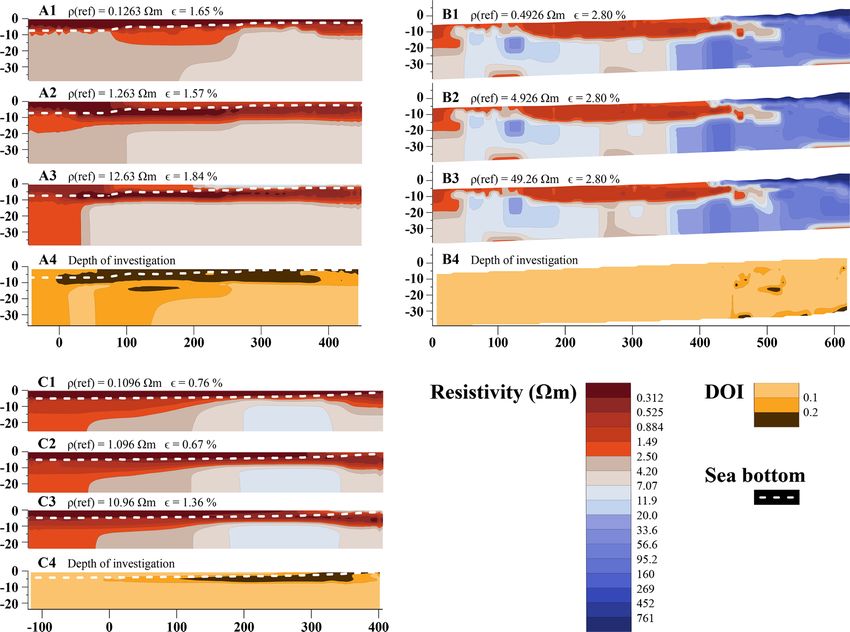
M. Paepen et al.: Combining resistivity and frequency domain electromagnetic methods to investigate SGD                        3543

mer ensures some overlapping with ERT on land, and the lat-         ments. For land ERT, reciprocals could not be collected be-
ter improves the resolution offshore, since the seawater layer      cause of time constraints related to the rising tide. The re-
is thinner in the low-tide conditions.                              peatability error was low, indicating data of good quality.
   Water-borne data were collected at high tide during a sin-       For the CRP inversion, the water layer was included using
gle day in 2018 (30 May). A total of two perpendicular and          the measured seawater conductivity (approximately 5 S m−1 )
three parallel profiles were obtained. The Syscal Pro Deep          and bathymetry (Loke, 2011). Note that the conductivity
Marine (IRIS Instruments) was used, combined with a 195 m           of the water layer is introduced as a soft constraint and is
long floating streamer of 13 graphite takeouts – 2 fixed cur-       not fixed during the inversion. This option was used to pre-
rent electrodes and 11 potential electrodes – spaced at a 15 m      vent the creation of artefacts of inversion, as these can oc-
interval. Using a reciprocal Wenner–Schlumberger configu-           cur when (potentially erroneous) strong constraints are intro-
ration, with the current electrodes in the middle of the set-up,    duced (Henderson et al., 2010; Caterina et al., 2014).
the simultaneous collection of 10 potentials was obtained for          Bad data points were filtered after a first inversion based
each current transmission (of 35 to 37 A). The streamer was         on the root mean square error (ERMS > 100 %). A robust in-
towed at a relatively constant speed (around 3.5 km h−1 ) by        version was carried out, using the floating-electrode-survey
a small rigid inflatable boat from the Flanders Marine Insti-       option for the marine profiles. Given the absence of robust
tute (VLIZ), which collected data continuously. In order to         error estimates, we relied on the convergence criterion typ-
correct for the influence of the highly conductive seawater         ically used for ERT to stop the inversion process (decrease
layer on the signal, a Garmin GPSMAP 188 Sounder system             of ERMS lower than 0.1 % between two iterations). The mean
was directly connected to the Syscal unit (obtaining coordi-        absolute error of all inverted models lies below 2.8 %.
nates and water depth), and seawater conductivity was sep-
arately recorded using a CTD (conductivity–temperature–             3.1.4   Inversion model appraisal
depth) diver.
   An additional marine survey was carried out on                   The resolution of resistivity profiles quickly decreases with
22 May 2019, allowing to measure three perpendicular pro-           depth. This is particularly true for marine profiles, as a large
files during low tide in front of De Westhoek. Again, the           portion of the current directly flows in the water layer. The
Syscal was used with the same set-up but with a cable of            inversion of marine data is thus subject to large uncertainty,
130 m. The 13 electrodes were spaced at 10 m, allowing for          and the quantitative interpretation of inversion results might
a better resolution yet sufficient penetration into the seabed.     be especially difficult (Day-Lewis et al., 2006). In our case,
                                                                    we are mostly interested in the relative variation of resistivity
Pre-processing                                                      indicating the presence of fresher water. To obtain informa-
                                                                    tion on how much the model is influenced by the inversion
In a first step, the raw marine data were checked, showing          parameters (bathymetry, starting model, etc.) and if reliable
the general trend in apparent resistivity. For the perpendicu-      resistivity variations are mapped, we propose an approach
lar high-tide profiles, e.g. K0HT (Fig. 2), an increase in resis-   based on the two-sided difference developed by Oldenburg
tivity is observed towards the beach. This is not only caused       and Li (1999) for estimating the depth-of-investigation (DOI)
by the decreasing thickness of the seawater layer – since           index. The DOI is an image appraisal tool which is often
other perpendicular CRP profiles made at Wenduine, Bel-             used to indicate which portions of the inversion model can
gium, (where possibly no or much less FSGD occurs; Fig. 2)          be interpreted. It is calculated based on two additional inver-
barely show this trend towards the land – but mainly due to         sions (ρinv,1 and ρinv,2 ) using the same dataset but for which
the outflow of fresh or brackish groundwater. The raw data          0.1 and 10 times the reference resistivity (ρref,1 and ρref,2 )
also display two bad acquisition channels (rho 6 and rho 7,         are imposed as a reference model:
Fig. 2) in all marine profiles (2018) caused by one damaged                  log ρinv,1 − log ρinv,2
electrode. These channels were removed from the datasets,           DOI =                            .                           (1)
                                                                             log ρref,1 − log ρref,2
reducing the sensitivity of the inversion models.
   The bathymetry was filtered to remove the noise effect           A low DOI value is obtained when resistivity structures in the
caused by the waves, by averaging the data. The echosounder         model are driven by the data and not by the inversion pro-
measurements of 2018 also comprise multiples. These were            cess which is influenced by the reference model. Although
calibrated with the known shore topography.                         a threshold between 0.1 and 0.2 on the DOI value is often
                                                                    used to delimit reliable zones of the image, this choice is
3.1.3   Processing                                                  subjective (Caterina et al., 2013). In addition, the DOI is di-
                                                                    rectly sensitive to the absolute value of resistivity and can
Both marine and land ERT data were inverted using the               thus yield high values even for consistently resistive or con-
RES2DINVx32 ver. 3.71.118 software. For marine data, po-            ductive structures. Therefore, we do not interpret the abso-
tentials were continuously measured, which prevents the es-         lute DOI value itself, even though it is very low throughout
timation of the error through stacking or reciprocal measure-       most inversion models but interpret it qualitatively with the

https://doi.org/10.5194/hess-24-3539-2020                                        Hydrol. Earth Syst. Sci., 24, 3539–3555, 2020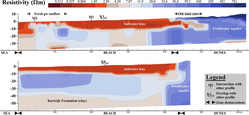
3544         M. Paepen et al.: Combining resistivity and frequency domain electromagnetic methods to investigate SGD

Figure 2. Raw resistivity data plots versus bathymetry. (a) Profile K0HT : strong resistivity increase towards the beach, mainly due to SGD.
(b) A perpendicular profile in front of the dunes of Wenduine, Belgium, where resistivity increases only slightly with decreasing water depth.

three respective inversions. We assume that we can make a                configurations with a coil spacing of 1.1 (PRP1), 2.1 (PRP2),
robust qualitative interpretation of the inversion model when            and 4.1 m (PRP4). Therefore, six different volume-related
all three inverted models show similar resistivity patterns.             apparent conductivities are recorded simultaneously. The
We are more careful in the evaluation if the models do not               depths at which the signal sensitivities are highest is am-
agree on the resistivity of certain zones. For marine data, the          biguous, since these depend on the specific subsurface con-
DOI is especially influenced by the thickness of the seawater            ductivity distribution. The approximate depths of investiga-
layer (bathymetry), which has a large effect on the calculated           tion provided by the six coil configurations are 0.5 (PRP1),
value.                                                                   1 (PRP2), 1.5 (HCP1), 2 (PRP4), 3 (HCP2), and 6 m (HCP4),
                                                                         but they have no physical meaning in this highly conduc-
3.2     Electromagnetic                                                  tive environment. To allow for a straightforward compari-
                                                                         son between datasets obtained with different coil configu-
3.2.1    Data acquisition                                                rations and instruments, these are here referred to as pseu-
                                                                         dodepths. The instrument’s operating frequency was 9 kHz,
Two different FDEM devices were used at De Westhoek.
                                                                         and elevation above the ground was 0.195 m. The sampling
Both have a short acquisition time and are relatively easy
                                                                         frequency was 8 Hz at an acquisition speed of approximately
to use in the intertidal zone. The DUALEM-421S has the
                                                                         8 km h−1 , rendering an in-line sampling spacing of approx-
advantage of a larger investigation depth compared to the
                                                                         imately 0.25 m. Survey lines were repeated in parallel lines
CMD-MiniExplorer, which only gives information of the up-
                                                                         at a spacing of approximately 5.5 m. Geographic coordinates
per 2 m.
                                                                         were logged using a Trimble R10 GNSS (global-navigation-
   The CMD-MiniExplorer (GF Instruments, s.r.o., Czech
                                                                         satellite-system) system (Trimble Navigation Ltd., Sunny-
Republic) is a portable multi-depth FDEM device which
                                                                         vale, California, USA).
measures apparent electrical conductivities (mS m−1 ). It was
used for mapping on 23 February 2018. The unit is relatively
small and, therefore, easy to use. The entire device is op-              3.2.2    Processing
erated by one person, who carries the 1.62 m long probe to-
gether with a Trimble GPS (Trimble Navigation Ltd., Sunny-               Basic processing of the DUALEM measurements was done
vale, California, USA). The system operates at 30 kHz and                following Delefortrie et al. (2014, 2015). The linear relation
contains three different receiver coils – dipole distances of            between the quadrature-phase (QP) component of the elec-
0.32 m (CMD1), 0.71 m (CMD2), and 1.18 m (CMD3). The                     tromagnetic field and the LIN ECa (McNeill, 1980) – used
horizontal-coplanar (HCP) configuration was used, giving a               in most commercially available FDEM equipment – is not
cumulative sensitivity of 0.5, 1.0, and 1.8 m, respectively, un-         valid in highly conductive environments, as it generally un-
der LIN (Callegary et al., 2007).                                        derestimates electrical conductivity (Fig. 3, left). Different
   Multiple-receiver FDEM data were recorded using                       from most studies, we converted the LIN ECa data to ro-
a DUALEM-421S instrument (DUALEM Inc., Milton,                           bust ECa (rECa), enabling qualitative FDEM data interpre-
Canada) mounted on a sled and towed by an all-terrain vehi-              tation in a highly conductive environment. We follow the
cle on 27 and 28 September 2018, after a very warm and dry               non-linear approach of Hanssens et al. (2019), in which rECa
summer. The device worked in HCP mode, which resulted in                 (mS m−1 ) data are calculated from the QP data to accurately
three HCP configurations with a coil spacing of 1 (HCP1),                estimate ECa at higher induction numbers (Fig. 3, right). Ul-
2 (HCP2), and 4 m (HCP4) and three perpendicular (PRP)                   timately, the data were interpolated in the software applica-

Hydrol. Earth Syst. Sci., 24, 3539–3555, 2020                                               https://doi.org/10.5194/hess-24-3539-2020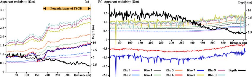
M. Paepen et al.: Combining resistivity and frequency domain electromagnetic methods to investigate SGD                        3545

tion Surfer 13 to a 2 m by 2 m grid, via natural neighbour          more difficult. The discharge zone will thus not be necessar-
interpolation.                                                      ily characterized by freshwater but rather by brackish water.

3.3    Interpretation
                                                                    4.1   FDEM
The inversion of resistivity data acts as a filter which tends
to blur the obtained image: the inverted resistivity is only        We started our investigation with the CMD-MiniExplorer
an estimation of the true resistivity. For this reason, it is       mapping at the location of one of the profiles of
difficult to directly relate an inverted-resistivity value to a     Lebbe (1981), K1, located 1 km east of the Belgian–French
specific value of the salinity or total dissolved solid (TDS)       border. The CMD-MiniExplorer mapping (Fig. 3, right, and
content. However, in this case, we have two well-identified         Fig. 4A) identifies the presence of FSGD close to the low-
extremes (freshwater in the dunes and seawater), together           water line, at K1, indicated by a decrease in the electrical
with a petrophysical model developed by Lebbe (1978, 1981,          conductivity. The FDEM data clearly demonstrate a zone
1999) for the western Belgian coastal plain, allowing for a         over 100 m wide. The outflowing water varies from very
semi-quantitative interpretation of resistivity. Archie’s law       brackish water to moderate saltwater; the conductivity is
(Archie, 1942) is used to estimate the pore water resistiv-         roughly between 350 and 650 mS m−1 , due to a mixture of
ity (ρw ):                                                          discharging fresh groundwater and seawater that infiltrated
                                                                    on the beach during high tide.
        ρb
ρw =       .                                                 (2)       To investigate lateral variation between the western and
        F                                                           eastern part of the study area, the intertidal zone was also
For sandy sediments at De Westhoek, Lebbe (1981) esti-              mapped with the DUALEM at the vicinity of the low-water
mated the formation factor (F ) to be 3.2. The bulk resistiv-       line. This map clearly demonstrates a northward shift of the
ity (ρb ), is deduced from ERT and CRP profiling and FDEM           zone of discharge from the east to the west (Fig. 4B–D).
mapping (given the scale of measurement, we assume that             From approximately 300 m east of the border, the discharge
the rECa value can approximate ρb ). Here, we propose a             zone is no longer visible from the EM data, since the dis-
semi-quantitative interpretation in salinity classes based on       charge is located below the low-water line. The DUALEM
relative variations in resistivity (and conductivity). Due to       was dragged on the beach in a sled, making the quality of
measurement errors, resolution, and inversion constraints,          the data higher compared to the MiniExplorer, which was
deducing the effective TDS would only be possible with a            carried by hand, making it difficult to maintain a constant
specific calibration of geophysical measurements based on           height above the surface during mapping. The water conduc-
ground truth data. We distinguish three main water quality          tivity, obtained with the DUALEM-421S, in the discharge
classes (saltwater, brackish water, and freshwater) to inter-       zone corresponds to a brackish-water type, confirming the
pret the geophysical data in the specific study area (De Moor       mixing of freshwater with salty water.
and De Breuck, 1969).
                                                                    4.2   Land ERT
4     Results and discussion
                                                                    Interpreted on its own, the conductivity variations observed
In the following paragraphs, we present the data and results        with FDEM could be related to lithological heterogeneities
for each of the used methods, starting with FDEM, then land         or the presence of near-surface features. Therefore, long land
and marine resistivity measurements. In the east of the study       ERT profiles (Fig. 5) covering the entire zone between the
area, FDEM data were acquired during two different sea-             low-water line and the dune area were collected. In the east
sons, allowing for an investigation of seasonal variability of      (Fig. 5, K1), we identify the freshwater aquifer located in the
the fresh-groundwater discharge. By comparing our results           dune area. The brackish water observed at −10 mTAW corre-
to previous observations, we can see how the freshwater–            sponds to remnants of seawater infiltration during the flood-
saltwater distribution has changed since the 1980s, due to          ing of an artificial tidal inlet, which started in 2004 and ended
a decrease of pumping in the nearby groundwater extraction          a few years ago. The downward movement of the denser sea-
facility. In the following, we will use a unique colour scale       water is hindered by the presence of a local clay lens, a pro-
to describe the results in all figures (except in Fig. 4): fresh-   cess that was closely monitored in previous studies (Vanden-
water occurs in zones with a resistivity higher than approx-        bohede et al., 2008b; Hermans et al., 2012). Along this pro-
imately 20  m (blue); saltwater has a resistivity lower than       file, there is a large saltwater lens on the beach. Underneath,
roughly 2.5  m (red); and brackish water leads to intermedi-       freshwater is flowing from the dunes towards the North Sea.
ate resistivities (light brown to light blue). In the case of the   The freshwater mixes with the saltwater, leading to the dis-
Belgian coast, the strong tides play a role in allowing salt-       charge of saltwater to brackish water during low tide on the
water to penetrate in the shallow sediment, and making the          lower beach. This is clearly visible on the land profile, close
detection of FSGD – based on resistivity and conductivity –         to the low-water line, where fresher water is seen near the

https://doi.org/10.5194/hess-24-3539-2020                                        Hydrol. Earth Syst. Sci., 24, 3539–3555, 2020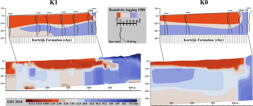
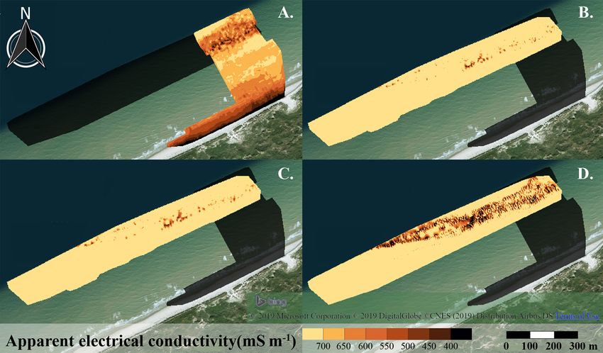
3546         M. Paepen et al.: Combining resistivity and frequency domain electromagnetic methods to investigate SGD

Figure 3. The CMD-MiniExplorer ECa mapping (left panel) versus rECa (right panel), both with CMD3, and a pseudodepth of approximately
1.8 m (23 February 2018). © Microsoft Corporation, DigitalGlobe, and CNES, 2019.

Figure 4. FDEM data. (A.) rECa (CMD-MiniExplorer) using CMD3, with a pseudodepth of approximately 1.8 m (23 February 2018).
(B.–D.) rECa (DUALEM-421S) using the HCP1, PRP4, and HCP4 configurations, respectively, providing pseudodepths of 1.5, 2, and 6 m
(27–28 September 2018). Note that another colour scale is used compared to the other figures. © Microsoft Corporation, DigitalGlobe, and
CNES, 2019.

surface, which corresponds to the zone identified by FDEM             underneath a saltwater lens from the dunes towards the sea.
measurements.                                                         Nevertheless, a striking difference on this profile is the ab-
   In the centre of profile K1 (Fig. 5), the groundwater ap-          sence of freshwater flowing upwards and discharging on the
pears to be brackish. Here, the thickness of the saltwater            lower beach. The saltwater lens, although becoming thinner
lens is at its maximum (15 m), while the bottom bound-                towards the low-water line, remains continuous. At the sea-
ary of the aquifer (thick clay layer) is located between              side of the profile, the underlying water is identified as fresh,
−25 and −30 mTAW. The lower resistivity is likely a re-               whereas it seems more brackish towards the dunes. This is
sult from the smoothness constraint inversion combined with           probably related to the higher resolution at depth when the
the lower resolution at depth as the more resistive freshwa-          conductive salt layer is thinner and not due to an actual vari-
ter is bounded by two conductive layers, leading to a lower           ation in salinity. On this profile, the clay layer (Kortrijk For-
inverted resistivity (Hermans and Paepen, 2020).                      mation) underlying the coastal aquifer is detected around
   There is a similar situation 1 km to the west, at the              −35 mTAW. The ERT data at the border gives the natural dis-
Belgian–French border (Fig. 5, K0), where freshwater moves            tribution of saltwater and freshwater, since the groundwater

Hydrol. Earth Syst. Sci., 24, 3539–3555, 2020                                           https://doi.org/10.5194/hess-24-3539-2020
M. Paepen et al.: Combining resistivity and frequency domain electromagnetic methods to investigate SGD 3547
Figure 5. ERT profiles in front of the De Westhoek nature reserve, perpendicular to the beach, at K1 (7 March 2018) and K0 (11 Octo-
ber 2018). Profile numbering based on Lebbe (1981), and the water depth is in mTAW (relative to the reference level of Belgium). Ground-
water: gw.
system is least affected by anthropogenic effects (extraction ner saltwater lens in the west, which increases the resolu-
facility) in this part of the study area. As a consequence, the tion of the inversion model. Modelling studies have shown
pore water is more resistive underneath the beach and further that the saltwater lens thickness is inversely related to the
offshore compared to K1. groundwater flux (Vandenbohede and Lebbe, 2006). Part of
the M1 profile (close to the middle) has a thicker lens com-
4.3 CRP pared to the zone around K1, while the water underneath K1
is more brackish, meaning that the fresh-groundwater flux
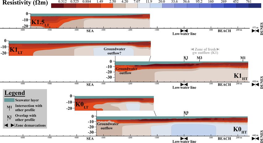
The land ERT profiles were extended by marine continuous is lower around K1. Also closer to the low-water line, re-
resistivity profiles collected at high tide, with an overlapping sistivity increases from K1 to K0 (Fig. 7, M2). East of K1,
zone of about 230 m (Fig. 6, K1HT and K0HT ). They confirm a more resistive body (light blue) is seen (Fig. 7, M3), and
the presence of brackish water below the saltwater and indi- this is also visible on the raw data. While on the eastern
cate that the discharge zone is not limited to the low-water side of the M3 profile (in front of the IWVA site), the re-
line but that it could extend towards the sea. In the east, weak sistivity is much lower compared to K1, which is compati-
saltwater migrates towards the seabed around 200 m in front ble with a lower fresh-groundwater flux (Vandenbohede and
of the low-water mark (Fig. 6, K1HT , light-red colour). Fur- Lebbe, 2006). The higher resistivity between the IWVA and
ther offshore, a marine profile, collected at low tide (Fig. 6, K1 can have multiple causes, which need further investiga-
K1LT ), confirms that brackish pore water can be seen up to at tion. The thickness of the overlying saltwater lens can have
least 550 m from the low-water line. It is mixed with saltwa- an effect, as well as the width of the beach (which is nar-
ter in the seabed, making it impossible to visualize FSGD at rower east of K1). Local hydrogeological heterogeneities can
the top of the seabed using resistivity measurements, but the have an influence too, since local clay lenses are present in
brackish groundwater is found relatively close to the seabed. the phreatic aquifer, which are difficult to identify in a saline
In the west, brackish groundwater is overlain by a thin environment due to their low resistivity. Maintaining the ca-
layer in which pore water is salty (Fig. 6, K0HT ). But the un- ble exactly parallel to the beach was also challenging; some
derlying brackish pore water is found closer to the seabed ap- measurement distortions are thus also possible.
proximately 250 m offshore the low-water line. The brackish To confirm the lateral variations in FSGD along this part
lens (Fig. 6, K0LT ) does not reach as far offshore compared of the coast, another perpendicular profile was collected fur-
to K1LT , perhaps due to different local hydrogeological and ther east (Fig. 6, K1.5LT ). Discharge seems stronger on K1LT
geological conditions. compared to K1.5LT , since the brackish aquifer extends fur-
To acquire information on the lateral variation, CRP pro- ther offshore. This observation is logical; K1.5LT is closer to
files parallel to the shore were collected during high tide. On the IWVA extraction site and, so, more affected by the wa-
the lower beach, the pore water resistivity increases from K1
towards K0 (Fig. 7, M1). This trend is partly due to the thin-
https://doi.org/10.5194/hess-24-3539-2020 Hydrol. Earth Syst. Sci., 24, 3539–3555, 2020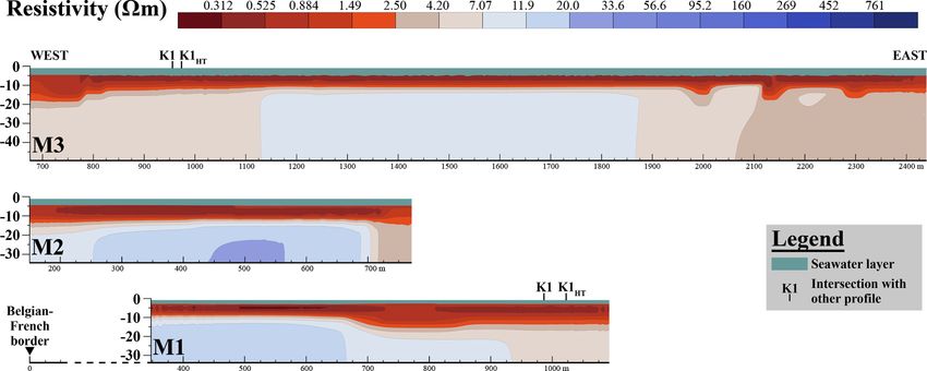
3548         M. Paepen et al.: Combining resistivity and frequency domain electromagnetic methods to investigate SGD

Figure 6. CRP profiles from De Westhoek, perpendicular to the beach, acquired on 30 May 2018 (K1HT and K0HT ) and 22 May 2019
(K1.5LT , K1LT , and K0LT ). Profile numbering based on Lebbe (1981), with HT and LT meaning high and low tide, respectively, and water
depth in mTAW (relative to the reference level of Belgium). Groundwater: gw.

Figure 7. CRP profiles parallel to the beach, taken during high tide (30 May 2018). The water depth in mTAW (relative to the reference level
of Belgium).

ter extraction reducing groundwater discharge. However, this            groundwater discharge might only occur at low tide, since the
should be further examined.                                             hydraulic gradient between land and sea is larger compared
                                                                        to the high tide); the electrodes of the streamer were spaced
4.4    Quality appraisal                                                closer during the low-tide survey (10 m compared to 15 m for
                                                                        the high-tide profiles); and fewer channels were obtained in
The resolution of the high-tide marine profiles is significantly        the high-tide survey (due to a bad electrode).
lower compared to that acquired during low tide, since it has              To validate the results of the ERT and CRP inversions,
a thicker seawater layer above the sea bottom; the portion of           we use the two-sided difference approach and the DOI, ad-
saltwater infiltrating in the seabed increases from low to high         ditionally computing the inversion for two different refer-
tide; it is collected in other dynamic conditions (significant

Hydrol. Earth Syst. Sci., 24, 3539–3555, 2020                                             https://doi.org/10.5194/hess-24-3539-2020
M. Paepen et al.: Combining resistivity and frequency domain electromagnetic methods to investigate SGD 3549 Figure 8. Validation of the inversion models at 1 km from the Belgian–French border. (A) K1HT marine profile; (B) K1 land ERT profile; (C) K1LT marine profile. HT and LT stand for high and low tide, respectively; ρ (ref) is the reference resistivity; and ∈ the absolute error. ence models. We show them for K1 (Fig. 8), but other pro- related to the thinner seawater layer. In summary, all profile files have similar results. For the land profile, all three in- types, although with different intrinsic resolutions, are sen- versions (Fig. 8, B1–3) look almost perfectly similar, with sitive enough to characterize the general salinity distribution practically all DOI values below 0.1 (Fig. 8, B4), indicat- in the studied zone. ing that observed structures are qualitatively contained in the data. For the profile at high tide (Fig. 8, A1–3), lateral varia- tions are also similar in the different inversion models, iden- 4.5 Seasonal variations tifying fresher pore water towards the beach. However, small variations are observed vertically around the sea bottom, cor- The MiniExplorer and DUALEM data were collected at the responding to DOI values above 0.2 (Fig. 8, C4), showing end of winter and beginning of autumn, respectively. The that the inversion is particularly sensitive to the bathymetry FSGD intensity around K1 is different in February (MiniEx- and the presence of the seawater layer. In this case, a low plorer) compared to October (DUALEM-421S), but the zone conductivity reference model will force some more resis- of discharge does not move (Fig. 4). During the former pe- tive features to appear closer to the sea bottom. As a conse- riod, the outflow of groundwater is clearly seen around K1 quence, brackish pore water seems closer to the sea bottom. at shallow depth (Fig. 4A), whereas in October, a large zone Whether this is actually the case or not cannot be elucidated of salty–brackish pore water is well visible at larger depth from our measurements, and the true extension of the FSGD (Fig. 4D) but only seen as individual spots of slightly lower zone cannot be delimited with certainty from the high-tide conductivity in the shallow subsurface (Fig. 4B and C). Ac- profile. For the low-tide profile (Fig. 8, C1–3), fewer dif- cording to the modelling results of Vandenbohede and Lebbe ferences are observed compared to those taken during high (2006), this seems to indicate that FSGD is stronger in winter tide, and the discharge zone is more clearly identified. This than autumn. This is likely due to the lower precipitation and is coherent with the higher resolution of the low-tide profile higher evaporation and evapotranspiration in summer, lead- https://doi.org/10.5194/hess-24-3539-2020 Hydrol. Earth Syst. Sci., 24, 3539–3555, 2020
3550         M. Paepen et al.: Combining resistivity and frequency domain electromagnetic methods to investigate SGD

Figure 9. Situation in 1980 versus 2018. Top panels: long normal resistivity logging along K1 and K0, modified from Lebbe (1981). Bottom
panels: 2018 land ERT profiles K1 and K0.

ing to smaller groundwater fluxes. In 2018, summer was par-           4.7   Advantages of the proposed methodology
ticularly dry in Belgium.
                                                                      By combining ERT, CRP, and FDEM, we have mapped
4.6    Long-term evolution                                            FSGD in 3D over a relatively large area, which comprises
                                                                      the dunes, the upper beach, the intertidal zone, and part of
Previous studies had shown the presence of freshwater under           the shelf. FDEM has allowed for imaging the lateral varia-
the saltwater lens in this study area but could not identify the      tion of the pore water conductivity in the upper metres of the
discharge zone. The identified saltwater lens at K1 is similar        intertidal zone, while ERT shows the vertical distribution of
in size to that observed in 1980, based on measurements of            freshwater and saltwater, which is extended offshore thanks
well logging on the beach (Lebbe, 1981; Fig. 9, top). How-            to CRP. Those results could not have been obtained with one
ever, the lens no longer extends to the sea, since the freshwa-       of the techniques alone or even with the combination of two
ter tongue reaches the surface nowadays on the lower beach.           of them. The previous conceptual model of the study area
This is probably an effect of the decreasing pumping trend            (Hermans et al., 2012) can be updated and extended offshore
of the IWVA exploitation site: the rate is now over 4.5 times         (Fig. 10).
lower compared to 1980, which has subsequently strength-                 For FDEM, the use of a robust estimation of the apparent
ened the groundwater discharge. Another explanation could             conductivity (rECa) is crucial in saline environments. Clas-
be that the logs collected in 1980 were not sufficient to detect      sical estimations with the LIN approximation would under-
the discharge zone, which could have occurred between the             estimate the ECa and reduce the observed contrasts, likely
two logs closest to the low-water line, in which case the salt-       leading to a wrong interpretation in terms of the salinity and
water lens would have remained relatively stable. However,            FSGD zone. Using this appropriate correction, we can more
this interpretation does not seem compatible with the newly           easily compare FDEM with ERT, which is crucial in com-
acquired CRP data which identify the presence of freshwa-             bined geophysical surveys.
ter further offshore. The shape and thickness of the saltwater           It is interesting to note that the presence of fresher water
lens at K0 have not changed much since 1980 (Fig. 9). The             is clearly visible on the raw CRP data as a gradual increase
lens becomes thinner towards the low-water line, but there            in the apparent resistivity (Fig. 2). The apparent resistivity
is no discharge on the lower beach, since FSGD is located             is the resistivity a homogeneous earth should have to provide
below this level. K0 is located furthest from the IWVA site,          with the same potential measurements and the same electrode
and no large extractions are known to occur on the French             configuration. It is not only influenced by the aquifer resis-
side of the border, so the effect caused by the decrease of the       tivity but also (and mainly) by the low seawater resistivity,
pumping is more limited.                                              explaining why apparent resistivity remains low, even in the
                                                                      presence of freshwater in the aquifer. The apparent resistiv-
                                                                      ity corresponds to a specific combination of four electrodes.
                                                                      With a spacing of 10 or 15 m between the electrodes, this cor-

Hydrol. Earth Syst. Sci., 24, 3539–3555, 2020                                           https://doi.org/10.5194/hess-24-3539-2020
M. Paepen et al.: Combining resistivity and frequency domain electromagnetic methods to investigate SGD 3551
Figure 10. Conceptual model. Based on the data presented in this study of Hermans et al. (2012) and de Verziltingskaart (De Breuck et al.,
1974). © Microsoft Corporation, DigitalGlobe, and CNES, 2019.
responds to an investigated volume with a minimum of 40 or 5 Conclusions
60 m in length. Therefore, the transition caused by changes in
the aquifer resistivity will be smoothed by the volume inves- In this contribution, we propose an innovative combination
tigated. A sharp freshwater–saltwater interface will thus ap- of land ERT and marine CRP together with FDEM mapping
pear as gradual in the raw data. Yet, possible zones of FSGD to characterize fresh-groundwater discharge. Electrical and
can be identified without inversion. If the seawater influence electromagnetic methods constitute practical tools in the in-
remains constant (which is true as long as its thickness re- vestigation of FSGD in coastal environments. The very high
mains similar), an increase of the apparent resistivity must spatial lateral resolution of FDEM combined with the verti-
correspond to an increase in the aquifer resistivity and thus a cal resolution of ERT allows for interpreting the presence of
decrease in its salinity. The apparent resistivity will also in- fresher water in 3D, while minimizing the field effort and the
crease when the bathymetry decreases but to a lesser extent acquisition time. By continuing ERT profiles seaward using
if the aquifer is salty (Fig. 2). CRP can therefore be used as a CRP, the surveyed area can be extended offshore to identify
fast exploration technique to locate zones of brackish–fresh discharge zones located below the low-water line, even in
pore water. Using this technique one can easily survey multi- rough areas characterized by large tidal ranges. While resis-
ple kilometres per day along the coastlines to detect the most tivity tomography is used to obtain a general 2D or pseudo-
vulnerable sites in terms of nutrient or contaminant leakage 3D model of the saltwater and freshwater distribution on
to the aquatic environment and a loss of freshwater. land, in the intertidal zone, and offshore, FDEM mapping
provides information on lateral variations. Since the data ac-
quisition is rapid and easy to use, this is perfectly suited for
https://doi.org/10.5194/hess-24-3539-2020 Hydrol. Earth Syst. Sci., 24, 3539–3555, 20203552 M. Paepen et al.: Combining resistivity and frequency domain electromagnetic methods to investigate SGD
the investigation of the intertidal zone and to fill the gap be- Competing interests. The authors declare that they have no conflict
tween ERT profiles that take longer to acquire. of interest.
As a standard output of commercially available (LIN)
FDEM instrumentation systematically underestimates ECa
values in highly conductive environments, the technique has, Acknowledgements. We want to thank the VLIZ for their logis-
to our knowledge, only rarely been used in the intertidal tical support in the marine surveys and the University of Liège
zone. However, limitations imposed by high conductive en- for lending the land ERT equipment. The authors would also like
to acknowledge Josue Chishugi, Nicolas Compaire, Tim Deck-
vironments can be overcome through a more robust interpre-
myn, Anja Derycke, Gaël Dumont, Hadrien Michel, Melissa Pri-
tation of the collected data (e.g. Hanssens et al., 2019). This
eto, Mizanur Rahman Sarker, Robin Thibaut, Bart Van Impe, Valen-
further extends the potential of FDEM to characterize FSGD tijn Van Parys, Jan Vermaut, and Nele Vlamynck for their help with
and SI in littoral zones. the field work. We also thank the editor, Gerrit H. de Rooij, and two
We demonstrate the ability of the proposed methodology anonymous reviewers for their comments which helped to improve
to characterize freshwater discharge occurring at De West- this paper.
hoek in the western Belgian coastal plain. In this area, FSGD
is present both below sea level and in the intertidal zone.
Land ERT profiles clearly identify the saltwater lens, under- Financial support. This research has been supported by the Fonds
lain by freshwater and originating from the infiltration of sea- Wetenschappelijk Onderzoek (research credit no. FWO1505219N)
water on the low slope shore and discharging on the lower and the Brilliant Marine Research Idea Grant 2018 of the Flanders
beach. CRP surveys further image the presence of brackish Marine Institute.
pore water and FSGD offshore. FDEM mapping in the inter-
tidal zone allows for characterizing lateral variations in the
discharge zone and locating where it becomes submarine. Review statement. This paper was edited by Gerrit H. de Rooij and
reviewed by two anonymous referees.
To our knowledge, this constitutes the first comprehensive
imaging of both the saltwater lens under the beach and the
shifting of FSGD seawards using geophysical techniques.
The discharge is most visible during low tide, since the
fresh-groundwater flux is higher compared to high tide. Low- References
tide conditions also allow for maximizing the resolution of
Archie, G. E.: The electrical resistivity log as an aid in deter-
both land and marine ERT, while enabling the acquisition of mining some reservoir characteristics, T. AIME, 146, 54–62,
FDEM data in the intertidal zone. High-tide data remain nec- https://doi.org/10.2118/942054-G, 1942.
essary to ensure some overlap with land ERT. The groundwa- Burnett, B., Bokuniewicz, H., Huettel, M., Moore, W. S.,
ter discharge seems to have a seasonal variability, with FSGD and Taniguchi, M.: Groundwater and pore water in-
being stronger at the end of winter compared to the beginning puts to the coastal zone, Biogeochemistry, 66, 3–33,
of autumn, since a warm and dry summer precedes the latter. https://doi.org/10.1023/B:BIOG.0000006066.21240.53, 2003.
The comparison of this new dataset to borehole logs from Burnett, W. C. and Dulaiova, H.: Estimating the dynamics
the 1980s shows that the decrease in groundwater pumping of groundwater input into the coastal zone via continuous
in the dunes has strengthened the freshwater outflow in the radon-222 measurements, J. Environ. Radioactiv., 69, 21–35,
https://doi.org/10.1016/S0265-931X(03)00084-5, 2003.
east of the area.
Burnett, W. C., Aggarwal, P. K., Aureli, A., Bokuniewicz, H., Ca-
ble, J. E., Charette, M. A., Kontar, E., Krupa, S., Kulkarni, K.
M., Loveless, A., Moore, W. S., Oberdorfer, J. A., Oliveira, J.,
Data availability. The data are accessible on the Marine Data Ozyurt, N., Povinec, P., Privitera, A. M. G., Rajar, R., Rames-
Archive (https://doi.org/10.14284/414, Paepen et al., 2020). sur, R. T., Scholten, J., Stieglitz, T., Taniguchi, M., and Turner, J.
V.: Quantifying submarine groundwater discharge in the coastal
zone via multiple methods, Sci. Total Environ., 367, 498–543,
Supplement. The supplement related to this article is available on- https://doi.org/10.1016/j.scitotenv.2006.05.009, 2006.
line at: https://doi.org/10.5194/hess-24-3539-2020-supplement. Callegary, J. B., Ferré, T. P. A., and Groom, R. W.: Vertical Spa-
tial Sensitivity and Exploration Depth of Low-Induction-Number
Electromagnetic-Induction Instruments, Vadose Zone J., 6, 158–
Author contributions. MP carried out the field work, processed the 167, https://doi.org/10.2136/vzj2006.0120, 2007.
resistivity data, performed the literature study, and wrote the first Cantarero, D. L. M., Blanco, A., Cardenas, M. B., Nadaoka, K.,
draft. DH and PDS processed the electromagnetic data. TH super- and Siringan, F. P.: Offshore Submarine Groundwater Discharge
vised the study and helped with the field work and the preparation of at a Coral Reef Front Controlled by Faults, Geochem. Geophy.
the draft manuscript. DH, PDS, KW, and TH edited and contributed Geosy., 20, 3170–3185, https://doi.org/10.1029/2019GC008310,
to the final paper. 2019.
Cardenas, M. B., Zamora, P. B., Siringan, F. P., Lapus, M. R.,
Rodolfo, R. S., Jacinto, G. S., Diego-McGlone, M. L. S.,
Hydrol. Earth Syst. Sci., 24, 3539–3555, 2020 https://doi.org/10.5194/hess-24-3539-2020You can also read