North SEAL: a new dataset of sea level changes in the North Sea from satellite altimetry - ESSD
←
→
Page content transcription
If your browser does not render page correctly, please read the page content below
Earth Syst. Sci. Data, 13, 3733–3753, 2021
https://doi.org/10.5194/essd-13-3733-2021
© Author(s) 2021. This work is distributed under
the Creative Commons Attribution 4.0 License.

          North SEAL: a new dataset of sea level changes in the
                   North Sea from satellite altimetry
           Denise Dettmering1 , Felix L. Müller1 , Julius Oelsmann1 , Marcello Passaro1 , Christian Schwatke1 ,
                                Marco Restano2 , Jérôme Benveniste3 , and Florian Seitz1
              1 Deutsches  Geodätisches Forschungsinstitut der Technischen Universität München (DGFI-TUM),
                                          Arcisstrasse 21, 80333 Munich, Germany
                                  2 SERCO, c/o ESRIN, Largo Galileo Galilei, Frascati, Italy
                         3 European Space Agency (ESA-ESRIN), Largo Galileo Galilei, Frascati, Italy

                              Correspondence: Denise Dettmering (denise.dettmering@tum.de)

                                   Received: 24 March 2021 – Discussion started: 29 March 2021
                             Revised: 30 June 2021 – Accepted: 30 June 2021 – Published: 2 August 2021

       Abstract. Information on sea level and its temporal and spatial variability is of great importance for various
       scientific, societal, and economic issues. This article reports about a new sea level dataset for the North Sea
       (named North SEAL) of monthly sea level anomalies (SLAs), absolute sea level trends, and amplitudes of the
       mean annual sea level cycle over the period 1995–2019. Uncertainties and quality flags are provided together
       with the data. The dataset has been created from multi-mission cross-calibrated altimetry data preprocessed with
       coastal dedicated approaches and gridded with an innovative least-squares procedure including an advanced out-
       lier detection to a 6–8 km wide triangular mesh. The comparison of SLAs and tide gauge time series shows good
       consistency, with average correlations of 0.85 and maximum correlations of 0.93. The improvement with respect
       to existing global gridded altimetry solutions amounts to 8 %–10 %, and it is most pronounced in complicated
       coastal environments such as river mouths or regions sheltered by islands. The differences in trends at tide gauge
       locations depend on the vertical land motion model used to correct relative sea level trends. The best consistency
       with a median difference of 0.04 ± 1.15 mm yr−1 is reached by applying a recent glacial isostatic adjustment
       (GIA) model. With the presented sea level dataset, for the first time, a regionally optimized product for the entire
       North Sea is made available. It will enable further investigations of ocean processes, sea level projections, and
       studies on coastal adaptation measures. The North SEAL data are available at https://doi.org/10.17882/79673
       (Müller et al., 2021).

1   Introduction                                                    adaptation measures. Furthermore, high-quality observation
                                                                    data on sea level provide a valuable contribution to the gen-
Sea level is one of the essential climate variables (ECVs) as       eral understanding of interactions and processes in the cli-
defined by the Global Climate Observing System (GCOS),              mate system. The coastal regions of the North Sea are in
and sea level rise is one of the most discussed topics in the       parts densely populated and of great economic significance.
context of global change. Risk assessment of potential threats      Especially for low-lying areas along large coastal stretches of
along the coasts by rising sea levels in connection with ex-        the German Bight, coastal protection measures, such as dike
treme events requires a solid data basis of sea level changes       building, are of paramount importance and associated with
over the past and predictions of its future evolution. A rise of    great efforts (Sterr, 2008).
the mean sea level (MSL) is accompanied by a higher proba-             The North Sea area is well equipped with measurement
bility of severe storm surges and floods (Wahl, 2017). Com-         systems monitoring sea level and its changes. Along the
prehensive and long time series of precise sea level obser-         coastlines many tide gauge (TG) stations provide valuable
vations are thus decisive for the development of appropriate

Published by Copernicus Publications.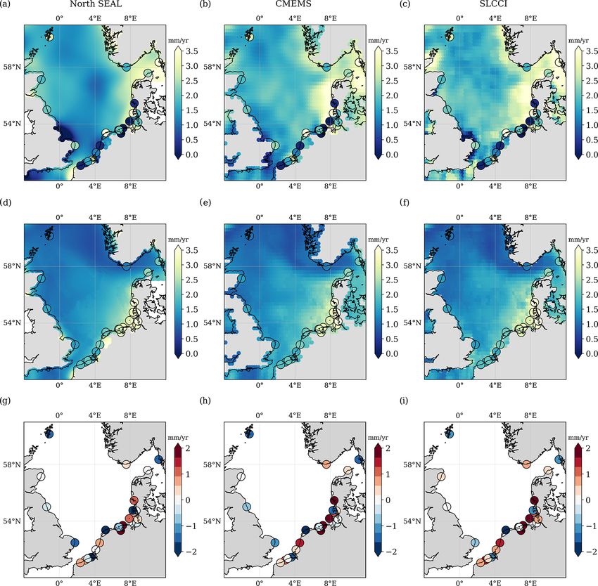
3734                                                                                            D. Dettmering et al.: North SEAL

data, in some cases for more than 100 years. In addition,           lantic for many years (Flather, 2000; Wakelin et al., 2003).
satellite altimetry can be used to monitor sea level offshore.      In contrast to observations, most models do have improved
Even if these time series are only about 25 years long, they        resolution and regular coverage. However, limitations may
are homogeneously distributed over the entire North Sea and         exist due to incomplete process descriptions or doubtful as-
provide the water stage in an absolute sense – in contrast to       sumptions, especially when no data assimilation is imple-
TG readings, which are referenced to fixed points on land and       mented. Observations and observation-based datasets like
are prone to vertical land motion (VLM). However, the tem-          North SEAL play an important role in validating and im-
poral resolution of satellite altimetry is quite sparse, and the    proving pure model simulations (Hermans et al., 2020; Tin-
creation of long-term and high-resolution sea level informa-        ker et al., 2020).
tion requires the combination of different satellite missions.         Observation data from satellite altimetry to monitor open-
Moreover, especially in the vicinity of coasts where land and       ocean sea level variations have been available since 1992. An
calm water may influence the radar echoes, the observation          early study using these data in the North Sea was published
data need to be carefully preprocessed.                             by Høyer and Andersen (2003). They assessed data from the
   Today, a few global altimetry-based sea level datasets are       TOPEX/Poseidon mission and compared them with TG data
available. One of them has been developed in the framework          with the aim of assimilating both data types into storm surge
of the ESA Sea Level Climate Change Initiative (SL_cci)             models. Already at that time, they found the root mean square
(Legeais et al., 2018), and another one is an operational prod-     error (RMSE) of merged altimetry and TG data to be signifi-
uct, computed by the Data Unification and Altimeter Com-            cantly lower than for the models. More recently, Sterlini et al.
bination System (DUACS) and provided by the Copernicus              (2017) analyzed satellite altimetry data to assess the causes
Marine Environment Monitoring Service (CMEMS) and the               for spatial variability of sea level trends in the North Sea.
Copernicus Climate Change Service (C3S) (Taburet et al.,            Within their study, they were able to address the spatial na-
2019). Global products include the North Sea, but they are          ture of the physical mechanisms that are responsible for sea
neither optimized for regional nor for coastal applications.        level change due to the availability of observation data over
Regional products from SL_cci covering the North Sea have           the open ocean. The altimetry data used were extracted from
recently shown enhanced coastal capabilities (Birol et al.,         the global DUACS DT2014 (Pujol et al., 2016) dataset pro-
2021; Benveniste et al., 2020), but they are limited to along-      vided by AVISO (Dewi Le Bars, personal communication,
track analysis of selected missions.                                23 April 2021). Due to the lack of coastal dedicated altime-
   Most studies investigating MSL changes in the North Sea          ter data preprocessing they focused on offshore regions only.
are based on country-wide TG analyses (e.g., Woodworth                 In recent years, the quality and quantity of altimetry data in
et al., 2009; Albrecht et al., 2011; Richter et al., 2012). In      the coastal zone have improved considerably (Cipollini et al.,
contrast, Shennan and Woodworth (1992) and later Wahl               2017): advanced radar waveform processing techniques have
et al. (2013) use long-term sea level measurements from a           been developed (e.g., ALES retracker, Passaro et al., 2014),
set of 30 TGs covering the entire North Sea coastline. Not          coastal dedicated geophysical corrections are available (e.g.,
surprisingly, the detected sea level trends and the interannual     GPD+ troposphere correction, Fernandes and Lázaro, 2016),
variability are not uniform along the coastline. For the period     and innovative altimeter instruments are providing data (e.g.,
1900–2011 and for the whole North Sea, Wahl et al. (2013)           SAR altimetry from Sentinel-3).
found an absolute MSL trend of 1.53 ± 0.16 mm yr−1 , which             In this study, a new gridded altimetry-based regional
increases to 4.00±1.53 mm yr−1 when only taking the period          sea level dataset for the North Sea is presented, named
1993–2009 into account. Later, Dangendorf et al. (2014a) ex-        North SEAL. It is based on long-term multi-mission cross-
tended this study to investigate the intra-annual to decadal-       calibrated data consistently preprocessed with coastal ded-
scale sea level variability in order to better understand the un-   icated algorithms and gridded to a 6–8 km wide triangular
derlying processes. More recently, Frederikse and Gerkema           mesh with innovative methods. The dataset enables advanced
(2018) demonstrated that the low-frequency variability in the       region-wide sea level studies and investigations of ocean pro-
seasonal deviations from annual mean sea level is mostly            cesses causing sea level variations on different spatial and
driven by wind and pressure. Information on open-ocean ar-          temporal scales.
eas was not derived in any of theses studies, since this cannot        The paper is structured as follows: Sect. 2 introduces the
be obtained from TG measurements. This is a critical limita-        study area and the input and validation data used. Section 3
tion, since from Benveniste et al. (2020) and Gouzenes et al.       describes the methods applied for data preprocessing, grid-
(2020) it is known that coastal sea level trends cannot al-         ding, and estimating derived parameters, i.e., trends and an-
ways be transferred to offshore regions. Moreover, sea level        nual amplitudes, which are considered to be of special inter-
changes differ significantly from region to region (Stammer         est for many users. Section 4 provides detailed information
et al., 2013).                                                      on the resulting dataset, such as time period, resolution, and
   Additional sources for studying the sea level and its vari-      data format, and Sect. 5 discusses the results. Section 6 com-
ation are physical ocean models. These have already been            pares the dataset with other existing altimetry datasets and
used in the North Sea, the European Shelf, and the North At-

Earth Syst. Sci. Data, 13, 3733–3753, 2021                                          https://doi.org/10.5194/essd-13-3733-2021
D. Dettmering et al.: North SEAL                                                                                             3735

with TG data. The article closes with a conclusion and infor-      2.3   Tide gauge data
mation about data availability.
                                                                   Monthly mean water level measurements of tide gauges are
                                                                   used for comparison and validation. The data are derived
2     Study area and input data                                    from the datum-controlled database of the Permanent Service
                                                                   of the Mean Sea Level (PSMSL) (Holgate et al., 2013) and
2.1    The North Sea
                                                                   from the German Wasserstraßen- und Schifffahrtsverwaltung
The North Sea is a semi-enclosed marginal sea of the North         des Bundes (WSV, 2013). The WSV provides TG data for
Atlantic Ocean situated on the northwestern European Shelf         the German Bight with measurements at semi-diurnal tidal
(Quante et al., 2016). It covers an area of about 560 000 km2      maxima and minima, i.e., at about 6 h resolution, which are
(970 by 580 km). It opens to the Atlantic through the Nor-         first smoothed with a 2 d running mean filter and then down-
wegian Sea in the north and has a second much smaller con-         sampled to monthly mean observations. Values are retained
nection through the English Channel in the south. Moreover,        which pass a 3-σ outlier test.
it is connected to the Baltic Sea in the east. Its mean depth         Among all available stations in the North Sea region, those
is around 94 m, with shallow areas less than 10 m deep in          are selected that contain at least 80 % valid measurements
the southern part and much deeper parts (up to 700 m) in the       during the study period (1995–2019), resulting in a total
Norwegian Trench area and parts of the Skagerrak. Sea level        of 54 stations. The same monthly averaged dynamic atmo-
dynamics in the North Sea are driven by various forcings,          spheric correction (DAC) is applied as used for the altimetry
namely tides (mainly semi-diurnal with a tidal range of up         data (Carrère and Lyard, 2003). To match the DAC with the
to 8 m), wind and atmospheric pressure, and heat and wa-           tide gauge records, among the nine closest points of the DAC
ter exchanges, as well as river runoff and forcing from open       grid the one that results in the highest variance reduction is
boundaries (Zhang et al., 2020). The influence of wind on          selected. TG data are not corrected for ocean tides, which
the sea level is large because the North Sea is very shallow       are assumed to be removed by monthly averaging. Remain-
(Dangendorf et al., 2014b). The general circulation pattern        ing influences from long-period tidal effects are assumed to
in the North Sea is mainly cyclonic. The water flows south-        have a smaller impact on the estimated trends than errors of
wards along the coastal areas of the British Isles, continues      ocean tide models would have directly at the coast.
eastwards and northwards along the coasts, and finally leaves
the basin as the Norwegian Coastal Current (Winther and Jo-
hannessen, 2006).                                                  2.4   Vertical land motion
   This study makes use of observation data collected in an        In order to make trends determined from TG data compara-
area between 4◦ W and 12.2◦ E longitude and 50 and 61◦ N           ble to absolute (i.e., geocentric with respect to an ellipsoid;
latitude, except the regions of the Irish Sea and the Baltic Sea   Gregory et al., 2019) sea level trends from satellite altimetry,
(Kattegat).                                                        the relative TG measurements need to be corrected for VLM.
                                                                      VLM can be estimated from point measurements (e.g.,
2.2    Satellite altimetry data                                    from Global Positioning System – GPS – observations) or
                                                                   from regional or global models. Since these estimates dif-
Satellite altimetry has been providing sea surface height in-
                                                                   fer significantly, data from different sources are used in
formation since the launch of the SeaSat mission in 1978.
                                                                   this study. Beside GPS data and glacial isostatic adjustment
But only since 1992 have at least two simultaneously mea-
                                                                   (GIA) models, the nonlinear effect of contemporary mass re-
suring satellites been in orbit, ensuring more reliable and
                                                                   distribution (CMR) on VLM is also applied.
precise height observations as well as improved data cov-
                                                                      GPS trends are derived from the dataset of the Nevada
erage and temporal resolution. This study includes almost
                                                                   Geodetic Laboratory (NGL) (Blewitt et al., 2016), which
all available missions since ERS-2 in 1995, namely TOPEX
                                                                   contains more than 17 000 vertical velocities (IGS08 refer-
(TP), ERS-2, Jason-1 (J-1), Envisat, Jason-2 (J-2), CryoSat-2
                                                                   ence frame). Only GPS VLM estimates from measurements
(CS-2), SARAL, Jason-3 (J-3), and Sentinel-3A/B (S3-A/B)
                                                                   with a minimum record length of 5 years between 1995 and
(ordered by launch dates). Data from the first phase of TP
                                                                   2019 are considered. To combine the VLM estimates with the
and from ERS-1 are not used because of doubts concerning
                                                                   TG trends, the nearest GPS station within a radius of 50 km
their trend stability (Mitchum, 2000; Kleinherenbrink et al.,
                                                                   around a TG is used.
2019). North SEAL comprises the period between May 1995
                                                                      GIA VLM estimates are taken from two different mod-
and May 2019 (see Fig. 1) and makes use of the latest data
                                                                   els. The first one, ICE-6G D (VM5a) (Peltier et al., 2018),
for all missions, updated by consistent external geophysi-
                                                                   was refined by geodetic constraints primarily by GPS ob-
cal model corrections and ITRF2014-based orbits whenever
                                                                   servations from the Jet Propulsion Laboratory (Desai et al.,
available; see Sect. 3.1 for more details.
                                                                   2009) over 1994–2012 and from other complementary ob-
                                                                   servations, such as very long baseline interferometry (VLBI)
                                                                   and Doppler Orbitography and Radiopositioning Integrated

https://doi.org/10.5194/essd-13-3733-2021                                         Earth Syst. Sci. Data, 13, 3733–3753, 2021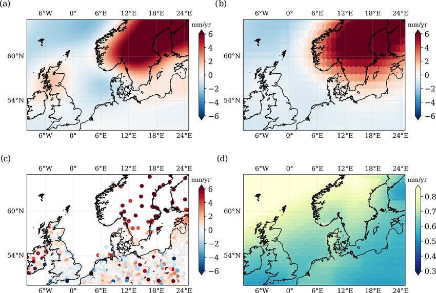
3736                                                                                         D. Dettmering et al.: North SEAL

Figure 1. Satellite altimetry missions used in this study.

by Satellite (DORIS) (Peltier et al., 2015). The model fit       2.5    External satellite altimetry products
to those observations was improved by modifications of the
                                                                 For validation purposes, North SEAL is compared with other
glaciation history. The second GIA VLM estimate is from
                                                                 gridded altimetry products available for the region. These
Caron et al. (2018) (hereinafter C18). The solution is based
                                                                 products are provided by CMEMS (Taburet et al., 2019) and
on an ensemble of 128 000 model runs. Among those, the
                                                                 SL_cci (Legeais et al., 2018). Both use a regular grid and
highest likelihood of parameters describing the ice history
                                                                 have a coarser spatial resolution of 0.25◦ . Given that the
and 1-D Earth structure was identified from an inversion of
                                                                 SL_cci dataset only lasts until 2015 (at the time of writing),
GPS and relative sea level data using Bayesian statistics. The
                                                                 all the following comparisons described in Sect. 3.4 are only
GIA estimate represents the expectation of the most likely
                                                                 performed over the period May 1995–December 2015.
GIA signal of the ensemble, and formal uncertainty estimates
are directly inferred from the Bayesian statistics.
   Ongoing changes in terrestrial water storage and mass         3     Methods
changes in glaciers and ice sheets cause elastic responses of
the Earth, which can result in nonlinear vertical movements.     Most of the methods applied in this study have been de-
These effects from CMR are not captured by GIA models and        veloped in the framework of the European Space Agency’s
only partially detected by GPS observations due to the rela-     Baltic+ Sea Level (ESA Baltic SEAL) project. Thus, de-
tive shortness of the record lengths. Using GRACE satellite      tailed information can be found in the Algorithm Theoretical
gravimetry observations, Frederikse et al. (2019) showed that    Baseline Document (ATBD) of that project (Passaro et al.,
associated time-varying solid Earth deformations can lead to     2020), in Passaro et al. (2021), and at http://balticseal.eu (last
very different trends (of the order of mm yr−1 ), depending on   access: 27 July 2021).
the time period considered during the last 2 decades. There-
fore, VLM estimates from GIA are supplemented with CMR-          3.1    Along-track data preprocessing
related land motions as used and distributed by Frederikse
                                                                 In order to generate monthly sea level anomaly (SLA) grids,
et al. (2020). This estimate is based on a blend of GRACE
                                                                 the altimetry along-track observations go through a chain of
and GRACE-FO observations during 2003–2018, as well as
                                                                 several preprocessing steps, including a retracking for con-
process model estimates, observations, and reconstructions
                                                                 ventional altimeters by the ALES retracker (Passaro et al.,
for the period 1900–2003 (see Frederikse et al., 2020, for a
                                                                 2014) and for SAR altimetry by the ALES + SAR retracker
detailed description of the datasets and sources used).
                                                                 (Passaro et al., 2020), an empirical adaption of the physical
   Figure 2 gives an overview of the applied VLM correc-
                                                                 ALES+ retracker (Passaro et al., 2018a) to SAR waveforms.
tions. There are some noticeable differences between the
                                                                 Moreover, a relative multi-mission cross-calibration (Bosch
two GIA estimates. In particular, the dipolar feature span-
                                                                 et al., 2014) referencing all altimetry missions used to the
ning from Scotland to the German Bight in the ICE-6GD so-
                                                                 TOPEX (and later to the Jason) data is performed. Sea level
lution (Fig. 2a) is much less pronounced in C18’s estimate
                                                                 anomalies are computed using the following equations.
(Fig. 2b). The linear CMR signal, which is computed over
1995–2019 (Fig. 2d), shows a non-negligible uplift signal of
about 0.7 mm yr−1 in the entire region of the North Sea.

Earth Syst. Sci. Data, 13, 3733–3753, 2021                                        https://doi.org/10.5194/essd-13-3733-2021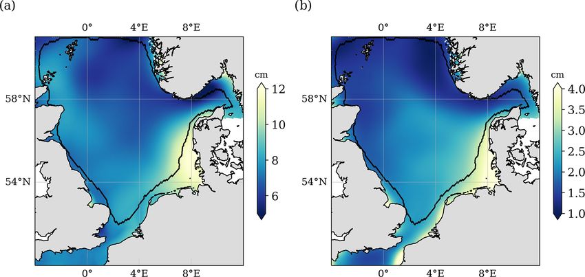
D. Dettmering et al.: North SEAL                                                                                                3737

Figure 2. VLM estimates used to correct relative sea level trends from TGs. GIA trends from (a) ICE-6G D (VM5a) and (b) Caron et al.
(2018). (c) GPS trend from the NGL solution. (d) Trend caused by contemporary mass redistribution over the period 1995–2019. Note that
the scale of (d) is much smaller than in the other plots.

                                                                        In a post-processing step, the along-track sea surface
                                                                     heights are cleaned from possible outliers by applying the
SSH = Horbit − (R + WT + DT + IONO + OT + SSB                        following four steps.
        + DAC + SET + PT + RC)                               (1)
                                                                        – Distance to coast: this is the elimination of observations
SLA = SSH − MSSH                                             (2)
                                                                          closer than 3 km to the coast (TOPEX: 5 km).
Here, Horbit , R, and MSSH mean the orbital height of the
satellite referred to the TOPEX/Poseidon ellipsoid, the al-             – Retracking flag: this is the elimination of corrupt obser-
timeter range, and the mean sea surface for reducing sea sur-             vations flagged based on the quality of waveform fitting
face heights (SSHs) to SLAs. In this study, the mean sea                  (retrack indicator ≥ 0.3 for conventional altimetry and
surface DTU15MSS (Andersen et al., 2016) is used, which                   ≥ 0.1 for SAR altimetry).
includes 20 years of data from the period 1992–2012. For
correcting atmospheric loading and wind effects, the DAC                – SLA threshold: this is the elimination of sea level
based on operational atmospheric products is used. Even if                anomalies exceeding the interval ±1.5 m.
corrections based on reanalysis data (i.e., DAC-ERA; Car-
rere et al., 2016) may improve the results for the early years,         – Contextual along-track outlier search: this is the elimi-
DAC is the only product currently available for the full pe-              nation of observations exceeding 3 times the mean ab-
riod under investigation. The other terms in Eq. (1) describe             solute deviation (MAD) from the local median (deter-
several geophysical and atmospheric effects, which are con-               mined from a moving median with a kernel size of 1 s).
sidered for SSH computation. They are listed in Table 1. The
sources of the orbital heights Horbit are provided in the Ap-          More details on this flagging are provided by Passaro et al.
pendix in Table A1.                                                  (2020).

https://doi.org/10.5194/essd-13-3733-2021                                            Earth Syst. Sci. Data, 13, 3733–3753, 2021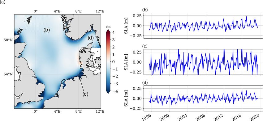
3738                                                                                                   D. Dettmering et al.: North SEAL

Table 1. Geophysical corrections applied to the along-track altimetry data.

         Correction                                 Model                             Reference                      Missions
         Dry troposphere (DT)                       VMF3                              Landskron and Böhm (2018)      all
         Wet troposphere (WT)                       VMF3                              Landskron and Böhm (2018)      S3-A/B
                                                    GPD+                              Fernandes and Lázaro (2016)    CS-2
                                                    GPD                               Fernandes et al. (2015)        all others
         Ionosphere (IONO)                          NIC09                             Scharroo and Smith (2010)      all
         Ocean tide (OT)                            FES2014 (ocean + loading)         Lyard et al. (2021)            all
         Dynamic atmospheric correction (DAC)       DAC (IB + MOG2D)                  CLS (2021)                     all
         Solid Earth tide (SET)                     IERS Conventions 2010             Petit and Luzum (2010)         all
         Pole tide (PT)                             IERS Conventions 2010             Petit and Luzum (2010)         all
         Sea state bias (SSB)                       MGDR                              Gaspar et al. (1994)           TP
                                                    ALES + SAR SSB                    Passaro et al. (2020)          CS-2, S3-A/B
                                                    ALES SSB                          Passaro et al. (2018b)         all others
         Radial correction (RC)                     MMXO18                            Bosch et al. (2014)            all

3.2    Gridding                                                               2. Iterative outlier detection based on estimated residuals
                                                                                 by applying a standard 3-σ criterion. The iterative out-
All observations passing the outlier elimination are in-                         lier search stops if no outliers are detected.
troduced into a least-squares gridding procedure (e.g.,
Koch, 1999). They are interpolated onto a triangular mesh                     3. Application of a one-sided t test by testing standardized
(geodesic polyhedron) in order to generate monthly grids                         residuals against quantiles of the Student’s distribution
with a spatial resolution between 6 and 8 km. The gridding                       (e.g., Koch, 1999). Observations that exceed the bound-
procedure mainly follows the process flow introduced by                          ary limit at a 99th percentile level of the Student’s dis-
Passaro et al. (2020) and Passaro et al. (2021). It is therefore                 tribution are excluded from the final coefficient estima-
only briefly described in the following text passages. Mean                      tion.
SLAs per grid node are computed by fitting an inclined plane
(h) to the along-track observations.                                        The monthly grids undergo a final check by removing sea
                                                                        level anomalies that exceed a threshold of ±2 m. For each
h(x, y) = c0 + c1 x + c2 y                                      (3)     grid node, the monthly mean SLAs are provided together
                                                                        with an estimate of the uncertainty. In addition, a quality flag
A local Cartesian coordinate system (x, y) is defined around            indicates if the node can be safely used or should be handled
each grid node, which represents the origin. The grid node              with care. This flag is allocated according to the standard de-
height is provided by the coefficient c0 , and c1 and c2 are            viation per node. If the standard deviation exceeds a specified
the slope coefficients. They are not used for the following             threshold and the node has less than 280 months of valid data,
processing. All along-track observations within a radius, the           it is labeled as “bad” quality (flag: 1). The threshold is set to
so-called cap size, of 150 km around each grid node are con-            the 90th percentile of all SLA standard deviations averaged
sidered. They are spatially averaged, whereby a Gaussian                over time.
weighting in consideration of their distance to the grid node
is applied. The minimum weight at the cap-size edge is set              3.3      Estimation of trend and amplitudes of the mean
to circa 10 %. Furthermore, uncertainty information is added                     annual sea level cycle
to the least-squares approach based on the MAD of sea level
anomalies per mission and month within a sub-area (0 to 6◦ E            The monthly SLA grids provide the basis for estimating a sea
and 54 to 58◦ N). The chosen area is free of topographic fea-           level trend per grid node as well as the amplitude and phase
tures. The MAD provides a rough estimate of the SLA noise               of the annual cycle. While a linear trend is fitted to the data,
level of a certain mission in a certain month. More informa-            the annual cycle amplitudes are obtained from half of the
tion is available in Passaro et al. (2020).                             differences of the months with the maximum and minimum
   Within the gridding procedure, the observations are fil-             multi-year monthly means. The uncertainties are based on
tered again in order to reject outliers from the estimation of          the combined uncertainties of these months.
the coefficients. This is done by performing a three-stage out-            Trend uncertainties are derived while accounting for au-
lier detection.                                                         tocorrelated errors in the data using maximum likelihood
                                                                        estimation (MLE). To identify the most appropriate noise
  1. Application of a standard 3-σ criterion to sea level               model required to accurately estimate the trend uncertain-
     anomalies within the cap size.                                     ties, we investigate the fit of a variety of different stochas-

Earth Syst. Sci. Data, 13, 3733–3753, 2021                                                  https://doi.org/10.5194/essd-13-3733-2021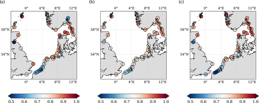
D. Dettmering et al.: North SEAL                                                                                              3739

tic noise model combinations as done in, e.g., Royston et al.          In contrast to trends and the annual cycle, correlations and
(2018). These are an autoregressive AR(1) noise model, a            rms are computed at the closest valid (i.e., with at least 280
power law plus white noise, a generalized Gauss–Markov              unflagged months of data available) altimetry node within
(GGM) plus white noise, a Flicker noise plus white noise,           a radius of 150 km. Correlations are derived from the de-
and an autoregressive fractionally integrated moving-average        trended altimetry and TG time series. We apply the quality
(ARFIMA(1,d,0)) model. For the considered domain, we                flag to the SLA dataset before computing correlations. This
find that on average (of all altimetry observations in the North    reduces the number of TG–altimetry pairs to 52. We also use
Sea) the AR(1) has the lowest mean (or median) values of the        the same number of TGs (52) for the comparison with other
Akaike information criterion (AIC; Akaike, 1998) and the            altimetry products.
Bayesian information criterion (BIC; Schwarz, 1978). Thus,             Next to correlations, we also analyze the rms difference
this model is selected to assess formal parameter uncertain-        of TG and altimetry time series in order to study the spread
ties. Uncertainties of the linear trend and the annual ampli-       between the data. To account for datum differences between
tude are given at the 95 % confidence interval.                     TGs and altimetry, offsets are removed from the difference
   For a more detailed description of the parameter estima-         time series. Three different solutions are computed: monthly
tion please refer to Passaro et al. (2021, 2020).                   detrended, monthly detrended and deseasoned, and annual
                                                                    detrended. In order not to distort the annual values by in-
3.4   Comparison of the data with tide gauges                       complete years, only the period from January 1996 to De-
                                                                    cember 2016 is used for all comparisons. To deseason the
To evaluate the performance of North SEAL, we compare               data, we subtract the multi-year monthly averages. Annual
absolute sea level trends and annual amplitudes derived from        averages are studied to compare the variability on interannual
satellite altimetry and TGs. Moreover, correlations and rms         timescales and to also assess the correctness of the represen-
between the two time series at TG locations are analyzed. It        tation of lower-frequency processes.
should be highlighted that taking the closest altimetry point
to a TG is not always necessarily the highest correlated or
                                                                    4     The North SEAL dataset
most representative observation. Thus, to match the altimetry
sea level data with the TG measurements, we follow the ap-
                                                                    All data are stored in NetCDF format and span a time period
proach of Oelsmann et al. (2021), which only uses the most
                                                                    from May 1995 to May 2019. It is provided on an unstruc-
highly correlated data in the comparison instead of taking
                                                                    tured triangular mesh characterized by nearly equally spaced
the altimetry observation closest to the TG. Oelsmann et al.
                                                                    grid node distances ranging from 6 to 8 km (geodesic poly-
(2021) showed that this approach ensures increased con-
                                                                    hedron) for the entire region of the North Sea between 4◦ W
sistency of along-track altimetry and TG observations and
                                                                    and 12.2◦ E and between 50 and 61◦ N with the exception of
enhances the agreement of trends. Here, 20 % of the best-
                                                                    the Irish Sea and the Kattegat.
correlated gridded altimetry data within a radius of 200 km
                                                                       The SLA grids are provided in monthly resolution.
around a TG are selected. This region is hereinafter called
                                                                    Data gaps due to missing observations or gridded SLAs
the zone of influence (ZOI). Time series of sea level are
                                                                    exceeding ±2 m are set to undefined. File names (i.e.,
computed from spatial averages of the altimetry data within
                                                                    YYYY_MM.nc) indicate year (YYYY) and month (MM).
the ZOI. Absolute sea level trend deviations between altime-
                                                                    All provided coordinates and height values are referenced
try and TGs are subsequently derived by subtracting the TG
                                                                    to the TOPEX ellipsoid. SLA data are referenced to the
measurements from the averaged altimetry data, whereby the
                                                                    DTU15MSS (Andersen et al., 2016). The file named North-
correction for VLM is applied.
                                                                    Sea_trend_and_annual_cycle.nc contains the sea level trends
   The uncertainties of absolute TG sea level trends u are
                                                                    and amplitudes of the annual cycle per grid node. Table 2
based on theq  combined uncertainties of the TG and the VLM
                                                                    lists all NetCDF variables included in the dataset.
trends (u = u2TG + u2VLM ). In order to compute uncertain-
ties of trend differences (for significance tests), the altimetry
                                                                    5     Results
uncertainties are also taken into account. Differences (and
their uncertainties) in the annual amplitudes are computed by       5.1    Sea level anomalies
subtracting the amplitudes from the individual altimetry and
TG time series and by computing the combined uncertainty            Figure 3 shows the mean SLA averaged over the observa-
of the annual amplitudes.                                           tion period of 24 years. In addition, three selected time series
   We note that the approach of using the ZOI significantly         at different locations in the North Sea are displayed. As de-
improves the comparability of sea level trends. Accordingly,        scribed in Sect. 3.1, the SLAs are referenced to the DTU15
the trend differences presented in Sect. 6 are on average           mean sea surface. Since the input data and time period of
about 20 % smaller when using the ZOI approach instead of           DTU15MSS (1992–2012) and North SEAL (1995–2019) are
taking the closest altimetry grid point.                            different, the SLAs do not average to zero everywhere. A ge-
                                                                    ographical pattern of negative offsets around 2 cm is visible

https://doi.org/10.5194/essd-13-3733-2021                                           Earth Syst. Sci. Data, 13, 3733–3753, 2021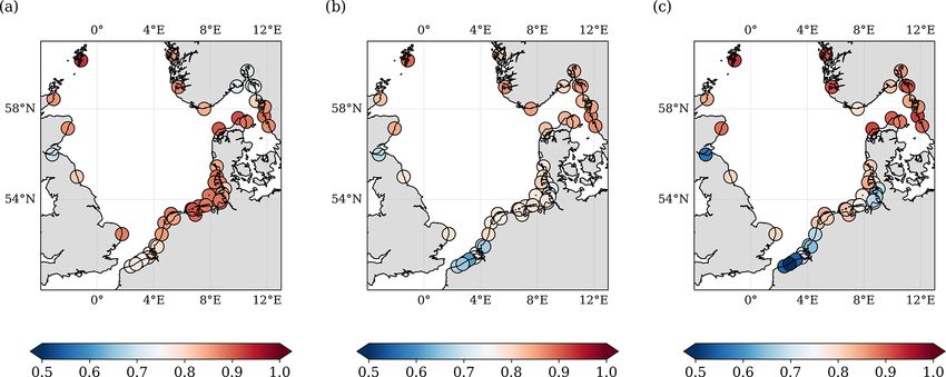
3740 D. Dettmering et al.: North SEAL
Table 2. NetCDF variables included in the dataset.
NetCDF variable Description Unit
Monthly SLA grids YYYY_MM.nc
lon Geographic longitude of grid node ◦
lat Geographic latitude of grid node ◦
time Day since 1 January 1985 00:00:00 (continuous) d
sla Sea level anomaly (SLA) m
sla_std_lsq Uncertainty of SLA per grid node resulting from the gridding procedure m
num_used_obs Number of observations used within the gridding procedure per grid node –
num_obs Number of theoretically available observations for gridding procedure per grid node –
qf_monthly_grid Quality flag resulting from the gridding procedure (bad: 1, good: 0) –
mss Mean sea surface height from DTU15MSS (Andersen et al., 2016) m
Trend grid NorthSea_trend_and_annual_cycle.nc
lon Geographic longitude of grid node ◦
lat Geographic latitude of grid node ◦
sla_trend Sea level trend over May 1995 until May 2019 m yr−1
sla_trend_unc Uncertainty of sea level trend (95 % confidence level) m yr−1
sla_annual_ampl Annual amplitude over May 1995 to May 2019 m
sla_annual_ampl_unc Uncertainty of annual amplitude m
sla_annual_ampl_max Month with maximum amplitude of the annual cycle –
sla_annual_ampl_min Month with minimum amplitude of the annual cycle –
qf_monthly_grid Quality flag resulting from gridding procedure (bad: 1, good: 0) –
in large parts of the coastal areas of the North Sea, especially 5.2 Sea level trends
along southern Norway and the coasts in the south. This ef-
fect is probably due to the use of a global MSS product that
Besides the mean sea surface, the temporal evolution of sea
uses a different set of retracked data and geophysical correc-
level is of great interest. In view of global change, the long-
tions. It has no influence on the time series analysis of SLA,
term change in particular is highly relevant for predicting fu-
in particular not on derived trends and annual amplitudes de-
ture sea levels and their impact for society and environment.
rived in this study. In fact, most of the affected regions are
Thus, as part of North SEAL, sea level trends are also pro-
edited when taking the quality flag (see Sect. 3.2) into ac-
vided. While the mean sea level trend between May 1995 and
count.
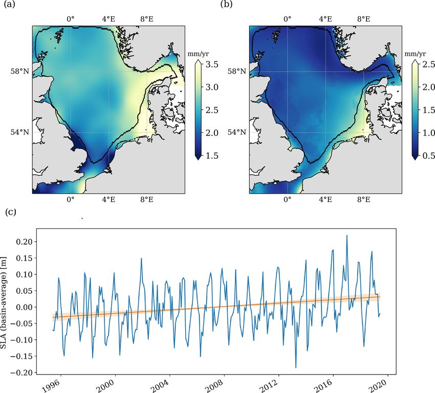
May 2019 in the North Sea amounts to 2.61 ± 0.95 mm yr−1 ,
The three SLA time series on the right-hand side of Fig. 3
the trend varies between 1.5 and 3.5 mm yr−1 over the region
show the temporal evolution of sea level for different grid
as illustrated in Fig. 4. The highest trends are observed in the
nodes. A distinct annual oscillation and interannual changes
German Bight and around Denmark, whereas significantly
are clearly visible for the three locations. Moreover, all three
lower trends are observed around the southern part of Great
curves show a rise of sea level.
Britain. Figure 4a and b include a black contour line. This
The monthly SLA time series displayed in Fig. 3b–d sug-
line confines the coastal areas flagged as decreased quality in
gest that the sea level variability differs strongly over the do-
the SLA dataset in the framework of the gridding procedure
main. In agreement with, e.g., Dangendorf et al. (2014a) and
(see Sect. 3.2). This flag is defined quite conservatively and
Wahl et al. (2013), the variance of the time series towards
tuned to provide optimal SLA time series. For trend compu-
the German Bight (Fig. 3c) strongly exceeds the variance ob-
tations, a rejection of the flagged areas is not necessary when
served at the Norwegian and British coastlines (Fig. 3b and
the trend uncertainties are taken into account in the course
d). Using long TG records, Dangendorf et al. (2014a) demon-
of the data analysis. When the flagged coastal regions are
strated that the sea level variability at the southern and east-
excluded, the overall trend for the North Sea changes only
ern coastlines of the North Sea is particularly dominated by
marginally to 2.60 ± 0.95 mm yr−1 .
westerly winds, which explains up to 80 % of the observed
Even with almost 2.5 decades of observation data, the
variability in these regions. The regional differences in vari-
trend uncertainties are still of the same order of magnitude
ability also influence the estimated sea level trends and their
as the trend itself. As visible from Fig. 4b, the trend uncer-
associated uncertainties, as with a length of 24 years the time
tainties vary between 0.5 and 2.5 mm yr−1 , with the small-
span is still relatively short.
est values in the northern part of the North Sea, especially
close to the Norwegian coast. The highest uncertainties can
Earth Syst. Sci. Data, 13, 3733–3753, 2021 https://doi.org/10.5194/essd-13-3733-2021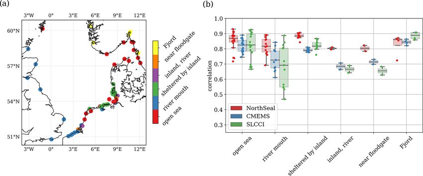
D. Dettmering et al.: North SEAL                                                                                               3741

Figure 3. Mean sea level anomalies over the period May 1995 to May 2019 in the North Sea (a) and three examples of time series of sea
surface anomalies at different locations (b–d).

be seen in the German Bight and at some smaller bays along           the estimated amplitudes of the annual cycle as derived from
the coasts of Great Britain and France. The particularly large       multi-year monthly means (see Sect. 3.3). The highest ampli-
uncertainties in the German Bight coincide with the afore-           tudes of more than 10 cm are visible in the German Bight and
mentioned larger sea level variability described by Dangen-          close to the Danish coasts. The signal is much smaller in the
dorf et al. (2014a) and may also be affected by poorer ocean         north of the region around Norway. Estimates of the annual
tide corrections in these areas.                                     amplitudes are much more accurate than the estimates of the
   The average trend of 2.61 ± 0.95 mm yr−1 differs from             trends. Uncertainties vary between 1 and 4 cm and amount to
the MSL trend of 4.00 ± 1.53 mm yr−1 observed by Wahl                approximately one-third of the signal itself.
et al. (2013) over 1993–2009. The difference is, however,
still within the limits of the confidence bounds. Deviations
between the trends may, on the one hand, be due to the dif-          6     Comparison with tide gauge measurements and
ferent periods of observation. On the other hand, the trend                external altimetry datasets
of Wahl et al. (2013) is based on TG observations and thus
                                                                     Detrended SLA time series of North SEAL are compared
may not unequivocally be compared to the sea level trend
                                                                     with measurements from TG stations and the alternative al-
from gridded altimetry data that are spatially distributed over
                                                                     timetry products from CMEMS and SL_cci (see Sect. 2.5)
the North Sea. In addition, the region was not exactly iden-
                                                                     using the methods described in Sect. 3.4. In order to be as
tical, as it extended further into the English Channel where
                                                                     consistent as possible, the analysis is performed for the over-
they found much smaller trends (1.32 ± 1.11 mm yr−1 ) than
                                                                     lapping time period of all three altimetry datasets (1995–
in the inner North Sea (4.59 ± 1.82 mm yr−1 ). Compared to
                                                                     2015).
the sea level trend of the North Sea over the last century of
1.53 ± 0.16 mm (Wahl et al., 2013), our study reveals a sig-
nificantly increased sea level trend over the past 2.5 decades.      6.1    Time series comparison
Again, however, the value from Wahl et al. (2013) is based
on TGs and not entirely comparable. In general, our observed         In order to assess how good North SEAL represents sea level
average trend is of the order of the global sea level trend of       variability on different timescales in comparison with TGs,
3.1±0.1 mm yr−1 (from 1995 to 2018) reported by Cazenave             correlations of the time series and their rms differences are
et al. (2018).                                                       analyzed. The median and mean correlation between North
                                                                     SEAL SLA and 52 TGs amounts to 0.86 and 0.85, respec-
                                                                     tively (Fig. 6a). The highest correlations (up to 0.93) are
5.3   Annual amplitudes
                                                                     found for the TGs at the Shetland Islands and along the
In addition to long-term changes in sea level, North SEAL            northern coast of Denmark. The lowest correlations appear in
allows for the analysis of seasonal variations. Figure 5 shows       small bays and fjords, e.g., the Firth of Forth (0.69) and the

https://doi.org/10.5194/essd-13-3733-2021                                           Earth Syst. Sci. Data, 13, 3733–3753, 2021
3742 D. Dettmering et al.: North SEAL Figure 4. Sea level trends from altimetry (a) and their associated uncertainties (b) for the period between May 1995 and May 2019. The black contour line confines the coastal regions flagged in the dataset. The curve in (c) shows the SLA time series averaged over the entire North Sea. The linear trend is 2.61 ± 0.95 mm yr−1 . Oslofjord (0.72). Low correlations are also observed along especially in the Oslofjord, North SEAL shows lower per- the coast of Belgium and the Netherlands at the mouth of the formance. This may be caused by a distance between the re- English Channel (Strait of Dover). spective grid node and the TG that is too large. This distribution is also visible in the correlations between Overall, with median and mean correlations of 0.86 the CMEMS/SL_cci products and TGs (Fig. 6b and c). Very and 0.85, respectively, North SEAL matches the TG mea- likely, some of those TGs in river mouths or smaller bays surements better than SL_cci (0.82/0.78) and CMEMS do not provide data that are representative for the sea level (0.79/0.78). Only for a minority of TGs are the correla- variations of the coastal or open ocean in their vicinity. Di- tions lower than for SL_cci (23.1 %) and CMEMS (11.5 %). viding all TG stations into different categories according to The average difference in correlation is about 0.06 for both their locations (Fig. 7) demonstrates that the majority of op- datasets (0.0651 for SL_cci; 0.0622 for CMEMS). This indi- timally located stations show correlations of around 0.8 or cates an average improvement in correlation between 8.4 % better, whereas stations located at fjords, rivers, or close to (CMEMS) and 10.5 % (SL_cci). floodgates show generally lower correlations. For stations The better performance close to the coast can be attributed located in river mouths the spread of correlation values is in large part to the consideration of quality flags in the North largest. On the other hand, stations sheltered by islands show SEAL SLA grids. They enable the selection of the closest high correlations with a small spread. For TGs at rivers and grid node with reliable SLA information and improve the near floodgates North SEAL clearly outperforms the other correlations with TG measurements by about 12 % on av- two products. Obviously, here, the quality flag successfully erage. Moreover, the flag led to the exclusion of two TG sta- prevents the use of inappropriate data. However, in fjords, tions for which no valid grid node could be found within a Earth Syst. Sci. Data, 13, 3733–3753, 2021 https://doi.org/10.5194/essd-13-3733-2021
D. Dettmering et al.: North SEAL                                                                                                      3743

Figure 5. Amplitudes of the annual cycle of the sea level (a) and associated uncertainties (b) for the period 1995–2019. The black contour
line confines the coastal regions flagged in the dataset.

Figure 6. Correlations between altimetry sea level anomalies and measurements of 52 TGs computed over a period of 20 years (1995–2015)
for three different altimetry datasets: (a) North SEAL, (b) CMEMS, and (c) SL_cci. The median correlations for all stations are 0.865 (North
SEAL), 0.789 (CMEMS), and 0.816 (SL_cci). Quality flags of North SEAL grids have been considered.

distance of 150 km (Oslo in Norway and Newhaven at the                  ries is included in the investigation. Table 3 shows the re-
south coast of Great Britain). Figure A1a in the Appendix               sults from these comparisons. The median rms values are all
shows the correlations between altimetry and TGs if the qual-           between 3 and 8 cm. North SEAL shows values of 4.9 cm
ity flags are not considered, i.e., if the SLA series at the grid       on a monthly scale (without annual signal) and 2.2 cm on
node closest to the TG is applied.                                      an annual scale. With this, it clearly outperforms the other
   In order to evaluate and quantify the consistency in sea             two products on a monthly scale. However, for the repre-
level variability, next to the correlations, the rms differences        sentation of lower-frequency processes, especially interan-
between altimetry and TG time series are computed and ana-              nual variability, the CMEMS product slightly outperforms
lyzed. This is done for all three altimetry datasets for monthly        the other datasets.
and for annual time series, both reduced by potential off-
sets and trends. In addition, a monthly deseasoned time se-

https://doi.org/10.5194/essd-13-3733-2021                                                Earth Syst. Sci. Data, 13, 3733–3753, 2021
3744 D. Dettmering et al.: North SEAL
Figure 7. Correlations between sea level variations from three different altimetry products and TG measurements depending on TG location
category.
Table 3. Comparison of sea level variability from altimetry (for North SEAL, CMEMS, SL_cci) and 52 TGs over 1996–2015. Differences
between altimetry and TGs are provided in terms of median rms in centimeters. The best altimetry solution in each case is marked in bold.
All time series are corrected for datum differences, and trends are reduced.
North SEAL CMEMS SL_cci
rms of monthly time series 5.07 6.24 7.51
rms of monthly deseasoned time series 4.86 5.77 7.26
rms of annual time series 2.20 1.94 2.31
6.2 Differences in trends and annual amplitudes Sea and are highest in the region of the Shetland Islands
and west of Norway. The main differences between the three
datasets can be seen in small bays (e.g., along the British
As described in Sect. 3.4, TG trends are corrected for VLM
coast), where North SEAL is characterized by higher uncer-
in order to make them comparable with the absolute sea level
tainties than the other two products. Based on the existing
trends from satellite altimetry. Figure 8 shows the absolute
data, it cannot be decided whether this behavior is caused by
sea level trends from three altimetry datasets and from TG
less correct trends or by more realistic uncertainties.
measurements (top row), their standard deviations (middle
The comparison of altimetry and TG trends (the latter
row), and the trend differences at the TG locations (bottom
corrected for VLM) reveals large discrepancies, while the
row). Since GPS information is not available for all TG loca-
uncertainties for both data types agree quite well. Trend
tions (see Sect. 2.4), the figure only contains 27 TGs.
differences reach up to 3.8 mm yr−1 with a median of
The trends from the three altimetry datasets show clear
−0.13 mm yr−1 and an rms of 1.40 mm yr−1 . Table 4 in-
regional differences. While all products show higher trends
dicates that the rms values for North SEAL are slightly
around Denmark, discrepancies are visible in the central
smaller than for the other two altimetry datasets (CMEMS:
North Sea. For large areas south of 56◦ N, the trends
1.42 mm yr−1 , SL_cci: 1.49 mm yr−1 ). However, since the
from SL_cci and (to a smaller extent) CMEMS are about
time period of about 20 years is still quite short for a reli-
1 mm yr−1 higher than the North SEAL trends. Likewise,
able trend estimation and since uncertainties of three differ-
both products show higher trends close to the coasts of
ent data types are involved (altimetry, TGs, and VLM), the
Denmark and Norway. These differences are up to about
trend differences for almost all locations are not statistically
1.5 mm yr−1 . However, none of these differences are signifi-
significant.
cant in view of the trend uncertainties.
Moreover, the values are dependent on the applied VLM
The trend uncertainties show similar geographic patterns
correction of the relative TG trends. Table 4 provides the
in all datasets. The lowest accuracies are found in the area of
rms of trend differences and the median bias between the
the German Bight. They improve towards the central North
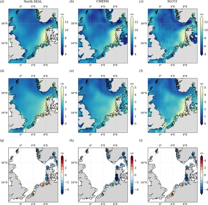
Earth Syst. Sci. Data, 13, 3733–3753, 2021 https://doi.org/10.5194/essd-13-3733-2021D. Dettmering et al.: North SEAL 3745 Figure 8. Absolute sea level trends over the period 1995–2015 (a–c) and associated uncertainties (d–f) for the three altimetry datasets (North SEAL, CMEMS, SL_cci) and TG measurements corrected for VLM. Differences in absolute sea level trends in TG locations (g–i). None of these differences are statistically significant. trends from altimetry and TGs. For consistency, these re- GIA-based VLM corrections compared to GPS corrections sults only refer to the 27 TGs that are co-located with a GPS could be caused by the relatively large maximum allowed station. Interestingly, implementing the GIA VLM correc- distance of 50 km between a TG and GPS station. Locally tion C18 (Caron et al., 2018) results in a lower deviation unequal VLM might introduce different signals at a GPS and of the trends than using local GPS information. For North TG location even over such distances. For example, two GPS SEAL, for example, the improvement is about 18 % in terms stations located on the island of Sylt (RANT and HOE2, in of rms. This VLM correction also outperforms the second the vicinity of TG Hörnum) indicate VLM estimates differ- GIA-based estimate from ICE-6G. The better performance of ing by more than 1 mm yr−1 , even though they are within https://doi.org/10.5194/essd-13-3733-2021 Earth Syst. Sci. Data, 13, 3733–3753, 2021
3746                                                                                                  D. Dettmering et al.: North SEAL

Table 4. Comparison of absolute sea level trends and annual amplitudes from altimetry (for North SEAL, CMEMS, SL_cci) and 27 TGs
(for which GPS data are available) over 1995–2015. Trend differences between altimetry and TGs are provided in terms of root mean square
(rms) difference and median bias in millimeters per year (mm yr−1 ; trend) and centimeters (annual amplitude). For each altimetry solution,
the best trend solution is marked in bold.

                                                   North SEAL                CMEMS                 SL_cci
                                                   rms         Bias         rms      Bias       rms         Bias
                          Trends
                          NGL(GPS)              1.4010      −0.134     1.4248      0.145     1.4905       0.424
                          C18                   1.1461       0.038     1.1577      0.234     1.3061       0.509
                          ICE-6G                1.3131       0.181     1.4312      0.096     1.5711       0.484
                          C18 + CMR             1.2755      −0.596     1.1514     −0.400     1.1580      −0.072
                          ICE-6G + CMR          1.3219      −0.421     1.3204     −0.475     1.3466      −0.099
                          Annual amplitudes     1.5981    −0.2499      2.3477     −1.4110    1.9140     −0.7305

a distance of only about 10 km. This could make a smooth                Bight (−6.0 cm). This value is just slightly larger than the
long-term GIA model make a better-suited correction. As can             combined uncertainty of 5.8 cm (95 % confidence level). The
be seen in Fig. 8g–i, the largest scatter of absolute sea level         German Bight is generally characterized by the largest an-
trends is observed in the German Bight, more precisely at the           nual amplitudes and largest uncertainties. Note that a neg-
offshore-located islands. Such areas could be more strongly             ative deviation means an underestimation of the amplitude
affected by local VLM than, for instance, the TG locations              in the altimetry dataset. For the whole domain, North SEAL
along the British coastlines.                                           shows the lowest absolute mean deviations of the annual cy-
   Adding the effect of CMR to GIA estimates influences the             cle of 1.3 cm (CMEMS: 1.8 cm; SL_cci: 1.5 cm) and the low-
agreement of the trends in different ways. We observe the               est rms difference of 1.6 cm compared to 2.3 and 1.9 cm (see
strongest improvement for SL_cci (for both rms and bias)                Table 3). This consolidates its coastal performance compared
and moderate improvement for the rms of CMEMS but with                  to the other altimetry products.
an increase in the bias. Likewise, the bias becomes larger for
North SEAL when the effect of CMR is added, and in this
case, the rms also increases (for either GIA-solution). The             7    Code and data availability
applied CMR correction generates a large-scale uplift sig-
nal of about 0.7 mm yr−1 over the domain (Fig. 2), which                The North SEAL dataset (i.e., monthly sea level anoma-
leads to an increased absolute sea level trend at the TG.               lies, sea level trends, and annual amplitudes) can be down-
This effect projects into the negative biases for North SEAL            loaded from SEANOE at https://doi.org/10.17882/79673
and CMEMS. The highest consistency between altimetry and                (Müller et al., 2021). The altimetry observations used
TGs is obtained for North SEAL when the TG measurements                 and all necessary atmospheric and geophysical correc-
are corrected using C18 VLM. Nevertheless, further inves-               tions are obtained from the Open Altimeter Database
tigations are worthwhile to understand why the CMR cor-                 (OpenADB) operated by DGFI-TUM (https://openadb.dgfi.
rection introduces pronounced biases for North SEAL and                 tum.de/en/, last access: 5 March 2021). Original altime-
CMEMS, while it improves the consistency for SL_cci. For                ter datasets are maintained by AVISO, ESA, NOAA, and
such studies, however, longer time series would be desirable            PODAAC. GPS vertical velocity estimates are provided
in order to reduce the trend uncertainties.                             by the NGL at the University of Nevada (http://geodesy.
   A comparison of the annual cycles among the altimetry                unr.edu, last access: 1 September 2020 – Blewitt et al.,
products and TG data reveals much better consistency than               2016). PSMSL tide gauge data are available at https://
in the case of sea level trends. Figure 9 shows the amplitudes          www.psmsl.org/data/obtaining/ (last access: 10 December
(top row), their uncertainties (middle row), and the discrep-           2020 – Holgate et al., 2013). Additional German tide
ancies between altimetry and TGs (bottom row). Overall, we              gauges were obtained from the Wasserstraßen- und Schiff-
find qualitatively similar patterns of the amplitudes and of            fahrtsverwaltung des Bundes (WSV) and are available
their uncertainties.                                                    on request through the Bundesanstalt für Gewässerkunde
   The difference between altimetry and TG amplitude is sig-            (BfG) (https://www.bafg.de, last access: 9 October 2020
nificant for only very few stations (three stations for North           – WSV, 2013). The CMEMS dataset (averaged DT-
SEAL and SL_cci, seven stations for CMEMS). The largest                 MSLA AVISO gridded altimetry data) is provided from
deviation is found for CMEMS at Dagebüll in the German                  AVISO (https://www.aviso.altimetry.fr, last access: 10 De-
                                                                        cember 2020). The SL_cci (Sea Level ECV v2.0) prod-

Earth Syst. Sci. Data, 13, 3733–3753, 2021                                               https://doi.org/10.5194/essd-13-3733-2021
D. Dettmering et al.: North SEAL 3747 Figure 9. Amplitudes of the annual cycle (a–c) and associated uncertainties (d–f) for the three altimetry datasets and TG data. Differences of annual amplitudes at TG locations are shown in (g–i). None of these differences are statistically significant. uct is available at https://doi.org/10.5270/esa-sea_level_cci- //zenodo.org/record/3862995#.X05RrIuxVPY, last access: IND_MSL_MERGED-1993_2015-v_2.0-201612 (last ac- 1 September 2020 – Frederikse et al., 2020). cess: 27 July 2020 – Legeais et al., 2018). The GIA A set of Python codes for novice coders, which has been dataset is available from JPL/NASA (https://vesl.jpl.nasa. developed in the framework of the ESA Baltic SEAL project, gov/solid-earth/gia/, last access: 1 September 2020 – can also be used for North SEAL. It provides tools to visu- Caron et al., 2018). The VLM is distributed at https:// alize the data and to convert it to other formats. It is avail- www.atmosp.physics.utoronto.ca/~peltier/data.php (last ac- able as a zipped file and can be downloaded from http: cess: 25 November 2020 – Peltier et al., 2018). The con- //balticseal.eu/outputs/ (last access: 27 July 2021). temporary mass redistribution is provided at Zenodo (https: https://doi.org/10.5194/essd-13-3733-2021 Earth Syst. Sci. Data, 13, 3733–3753, 2021
3748                                                                                           D. Dettmering et al.: North SEAL

8   Conclusions                                                        With North SEAL, for the first time, a regionally opti-
                                                                    mized sea level dataset for the entire North Sea is available.
This paper presents the new dataset North SEAL of monthly           Even though the length of the time series is still much shorter
gridded sea level heights in the North Sea over the period          than some of the TG records in the region, the data offer
1995–2019. North SEAL contains sea level anomalies, long-           the possibility to investigate sea level changes – not only in
term mean sea surface heights (DTU15MSS), uncertainty es-           coastal but also in offshore areas. This enables basin-wide
timates, and quality flags on a triangular 6–8 km mesh. In          studies of physical processes driving sea level variability,
addition, derived linear sea level trends and amplitudes of         such as the impact of atmospheric wind and pressure forcing,
the annual cycle are provided per grid node. An updated             as has already been done based on the Baltic SEAL dataset,
mean sea surface optimized for use together with the sea            which Passaro et al. (2021) used to study the connection be-
level anomalies of North SEAL is subject to future work.            tween sea level anomalies in different areas of the Baltic Sea
North SEAL has been created from 24 years of multi-mission          and the North Atlantic Oscillation. North SEAL will enable
cross-calibrated altimetry data, which were carefully prepro-       similar studies as that of Dangendorf et al. (2014a) based
cessed and optimized for coastal applications. Along-track          on a consistent dataset for offshore and coastal areas at a
data were gridded using the innovative procedure developed          higher spatial scale. Moreover, an improved determination
within the ESA Baltic SEAL project.                                 of sea level signatures of coastal currents can be expected.
   Comparison with existing global altimetry products and           This is something that was, until now, only possible using
with TG observations revealed an improved performance,              along-track data (e.g., Passaro et al., 2015; Birol and Dele-
with average correlations between SLA and TG time series            becque, 2014). In addition, the new dataset can help to vali-
of 0.85. Monthly deseasoned time series result in a median          date and improve ocean or climate models. Through both the
rms of the altimetry–TG difference time series of 4.9 cm,           improved process understanding and the improved modeling,
while the median rms in the case of annual mean values is           North SEAL can also be beneficial for sea level projections.
2.2 cm. These values clearly outperform other existing al-          It provides an observational basis to better estimate the time
timetry products on a monthly scale, but North SEAL can             of emergence of projected sea level change above observed
still be improved to better represent interannual variabil-         variability and for the planning of adaptation and coastal pro-
ity. The median trend differences with respect to TGs are           tection measures.
0.04±1.15 mm yr−1 (C18 VLM). Since the investigation pe-               North SEAL is provided as an updated version at irregular
riod is relatively short, the uncertainties are still too high to   intervals to incorporate the latest observations, reprocessed
see statistically significant trend differences. The mean devi-     altimetry data, and the most up-to-date geophysical models.
ation of the annual amplitude with respect to TG observations
is 1.3 cm.

Earth Syst. Sci. Data, 13, 3733–3753, 2021                                          https://doi.org/10.5194/essd-13-3733-2021
You can also read