Residential Property Price Index in Japan: Discussion in Methodology and Data Sources - International Conference ...
←
→
Page content transcription
If your browser does not render page correctly, please read the page content below
International Conference on Real Estate Statistics, Eurostat 2019

Residential Property Price Index in Japan: Discussion in
             Methodology and Data Sources
                      Chihiro Shimizu∗ and W. Erwin Diewert†

                                  This Draft: Feb 3, 2019

                                             Abstract
          Fluctuations in housing prices have substantial economic impacts. Thus, it is es-
      sential to develop housing price indexes that can adequately capture housing market
      trends. However, construction of such indexes is very difficult due to the fact that res-
      idential properties are heterogeneous and do not remain at constant quality over time
      due to renovations and depreciation of the structure. In order to improve the quality
      of housing price statistics Eurostat published the Residential Property Price Indices
      Handbook in 2012. In constructing a housing price index, one has to make several
      non-trivial choices. One of them is the choice among alternative estimation methods,
      such as repeat-sales regression, hedonic regression, etc. There are numerous papers on
      this issue, both theoretical and empirical. Shimizu et al. (2010), for example, conduct
      a statistical comparison of several alternative estimation methods using Japanese data.
      However, there is another important issue which has not been discussed much in the lit-
      erature, but which has been regarded as critically important from a practical viewpoint:
      the choice among different data sources for housing prices. There are several types of
      datasets for housing prices: datasets collected by real estate agencies and associations;
      datasets provided by mortgage lenders; datasets provided by government departments
      or institutions; and datasets gathered and provided by newspapers, magazines, and
      websites. Needless to say, different datasets contain different types of prices, including
      sellers’ asking prices, transaction prices, valuation prices, etc. With multiple datasets
      available, one may ask several questions. Are these prices different? If so, how do they
      differ from one another? Given the specific purpose of the housing price index one
      seeks to construct, which dataset is the most suitable? Alternatively, with only one
      dataset available in a particular country, one may ask whether this is suitable for the
      purpose of the index one seeks to construct. The paper discusses alternative methods
      for obtaining constant quality housing price statistics and alternative data sources in
      the Japanese context.
          Key Words : House price indexes; hedonic price indexes; repeat sales price in-
      dexes; aggregation bias; housing depreciation; land and structure components; flexible
      functional forms; Fisher ideal indexes.
          JEL Classification : C2, C23, C43, D12, E31, R21.

  ∗ Nihon University in Tokyo & MIT Center for Real Estate. Expert member, Statistics Commission of

Cabinet Office in Japan, E-mail: shimizu.chihiro@nihon-u.ac.jp.
  † The University of British Columbia & The University of New South Wales.

                                                 1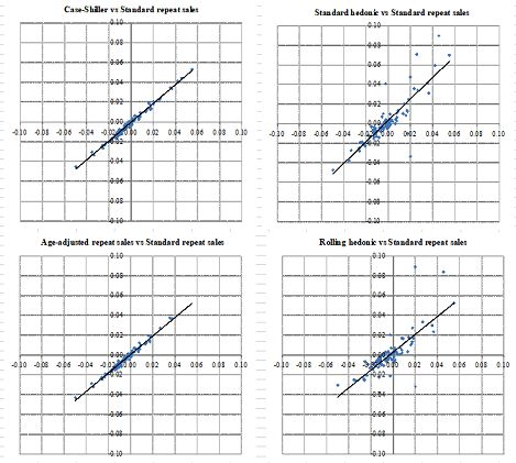
1      Introduction
  Fluctuations in real estate prices have substantial impacts on economic activities. In
Japan, a sharp rise in real estate prices during the latter half of the 1980s and its decline in the
early 1990s led to a decade-long stagnation of the Japanese economy. More recently, a rapid
rise in housing prices and its reversal in the United States triggered a global financial crisis.
In such circumstances, the development of appropriate indexes that allow one to capture
changes in real estate prices with precision is extremely important, not only for policy makers
but also for market participants who are looking for the time when housing prices hit bottom.
Recent research has focussed on methods of compiling appropriate residential property price
indexes. The location, maintenance and the facilities of each house are different from each
other in varying degrees, so there are no two houses that are identical in terms of quality.
Even if the location and basic structure are the same at two periods of time, the building
ages over time and the houses are not identical across time. In other words, it is very
difficult to apply the usual matching methodology (where the prices of exactly the same item
are compared over time) to housing.
    As a result, one may say that the construction of constant quality real estate price indexes
is one of the most difficult tasks for national statistical agencies. In order to address these
measurement problems, Eurostat published the Residential Property Price Indices Handbook
in 2012. Chapters 4 through 7 of this Handbook are devoted to methods for constructing
constant quality price indexes.1 Chapter 8 deals with the problems associated with de-
composing an overall property price index into land and structure components,2 Chapter
9 discusses data sources and Chapter 10 reviews methods currently used by private and
government index providers.
    In the wake of the release of this Handbook, how should different countries construct res-
idential property price indexes? With the start of the Residential Property Price Indices
Handbook project, the government of Japan set up an Advisory Board through the Min-
istry of Land, Infrastructure, Transport, and Tourism (MLIT) and is proceeding with the
development of a new Japanese official residential property price index. This paper out-
lines the results of the advisory board’s ongoing review with regard to the development of a
residential property price index for Japan.3
  Sections 2 and 3 below summarize the results of deliberations by the Advisory Board
regarding residential property price indexes estimation methods. The material in these
sections is based on the paper by Shimizu, Nishimura and Watanabe (2010). Section 4
summarizes the results of deliberations regarding selection of data sources. Section 5 then
    1 Chapters 4-7 deal with the following methods: stratification or mix adjustment methods, hedonic

regression methods, repeat sales methods, and appraisal based methods.
    2 This decomposition is required in order to construct the national accounts for a country.
    3 The Advisory Board was set up by the Ministry of Land, Infrastructure, Transport and Tourism,

with the participation of the Bank of Japan, Financial Services Agency, Ministry of Justice (which is the
department responsible for the land registry), Statistics Japan (the department responsible for the consumer
price index), the Cabinet Office (the department responsible for SNA), the Japan Association of Real Estate
Appraisers and various realtor associations. As of 2013, the Advisory Board also began developing a official
Commercial Property Price Index in addition to developing the Residential Property Price Index.

                                                     2
outlines the results of analysis of an outstanding issue: methods for separating housing prices
into land and building component prices. Finally, section 6 summarizes what kind of index
the government of Japan intends to publish as an official Residential Property Price Index.4

2      Alternative Methods for Constructing Residential Prop-
       erty Price Indexes
2.1         Introduction: The Two Main Methods for Making Quality Ad-
            justments
    A key starting point in estimating a housing price index is to recognize that each property
at each point in time is a unique item. Even if the location and basic structure of the housing
unit are the same at two points in time, depreciation, alternative maintenance policies and
renovations alter the quality of the structure so that like cannot be precisely compared with
like. Given this special feature of houses and hence housing services, an important task for
researchers is to make adjustments for differences in quality. There are two methods widely
used by practitioners and researchers: the hedonic method and the repeat sales method. A
primary purpose of the paper by Shimizu, Nishimura and Watanabe (2010) was to compare
these two methods using a unique dataset that we they compiled from individual listings in
a widely circulated real estate advertisement magazine.
    Previous studies on house price indexes have identified several problems for each of the two
main methods for quality adjustment. The real estate literature has identified the following
problems with the repeat sales method:

     • The repeat sales method may suffer from sample selection bias because houses that
       are traded multiple times have different characteristics than a typical house.5

     • The repeat sales method basically assumes that property characteristics remain un-
       changed over time. In particular, the repeat sales method neglects depreciation and
       possible renovations to the structure.6

    On the other hand, the hedonic method suffers from the following problems:

     • The failure to include relevant variables in hedonic regression may result in estimation
       bias.7

    4 Sections 2 and 3 draw heavily on the paper by Shimizu, Nishimura and Watanabe (2010).
    5 See Clapp and Giacotto (1992). Repeat sales that occur in very short time periods are often not regarded
as “typical” sales. In particular, the initial sale may take place at a below market price and the subsequent
rapid resale takes place at the market price, and this phenomenon may lead to an upward bias in the resulting
repeat sales price index. Of course, this source of upward bias is partially offset by the downward bias in the
repeat sales method due to its neglect to make a quality adjustment for the depreciation of the structure.
    6 See Case and Shiller (1987) (1989), Clapp and Giaccotto (1992) (1998), Goodman and Thibodeau

(1998), Case, Pollakowski, and Wachter (1991) and Diewert (2010).
    7 See Case and Quigley (1991) and Ekeland, Heckman, and Nesheim (2004).

                                                      3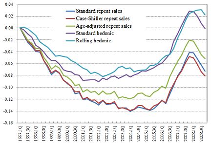
• An incorrect functional form may be assumed for the hedonic regression model.8

    • The assumption of no structural change (i.e., no changes in parameters over time) over
      the entire sample period may be too restrictive.9

 Given that true quality adjusted price changes are not observable, it is difficult to say
which of the two measures performs better. However, at least from a practical perspective,
it is often said that the repeat sales method represents a better choice because it is less
costly to implement.10 However, as far as the Japanese housing market is concerned, there
are some additional concerns about the repeat sales method:

    • The Japanese housing market is less liquid than those in the United States and Euro-
        pean countries, so that a house is less likely to be traded multiple times.11

    • The quality of a house declines more rapidly over time in Japan because of the short
      lifespan of houses and the fact that — for various reasons — renovations to restore the
      quality of a house play a relatively unimportant role. This implies that depreciation
        plays a more important role in the determination of house prices, which is not taken
        into account in the repeat sales method.

  Given these features of the Japanese housing market, Shimizu, Nishimura and Watanabe
(2010) argued that, at least in Japan, the hedonic method is a better choice. Another
important advantage of the hedonic method over the repeat sales method is that the former
method can lead to a decomposition of the sales price of a property into land and structure
components. This decomposition cannot be obtained using the repeat sales method.
   In the remainder of this section, we will discuss the various variants of the hedonic regres-
sion and repeat sales models that are used in practice.

2.2        The Standard Hedonic Regression Model
  We begin with a description of the standard hedonic regression model. Suppose that we
have data for house prices and property characteristics for periods t = 1, 2, . . . , T . It is
assumed that the price of house i in period t, Pit , is given by a Cobb-Douglas function of
the lot size of the house, Li , and the amount of structures capital in constant quality units,
Kit :
                                                            β
                                               Pit = Pt Lα
                                                         i Kit                                              (1)
   8 See   Diewert (2003a) (2003b).
   9 See   Case, Pollakowski, and Wachter (1991); Clapp and Giaccotto (1992) (1998), Shimizu and Nishimura
(2006) (2007) and Shimizu, Nishimura and Watanabe (2010).
    10 See Bourassa, Hoesli and Sun (2006). The hedonic method requires information on property charac-

teristics whereas the repeat sales method does not require any characteristics information. However, this
informational advantage of the repeat sales method is offset by its informational sparseness disadvantage;
i.e., repeat sales information may be so infrequent so as to make the construction of accurate price indexes
impossible. Moreover, unless the sample selection bias exactly offsets the depreciation bias, we can say that
the repeat sales method is definitely biased whereas we cannot definitely assert that the hedonic method is
biased.
    11 This may be partly due to the presence of legal restrictions in Japan on reselling a house within a short

period of time.

                                                       4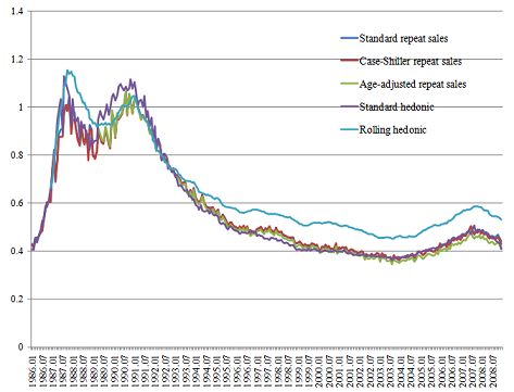
where Pt is the logarithm of the quality adjusted house price index for period t and α and β
are positive parameters.12 It is assumed that housing capital, Kit , is subject to generalized
exponential depreciation so that the housing capital in period t is given by

                                          Kit = Bi exp[−δAλit ]                                         (2)

where Bi is the floor space of the structure, Ait is the age of the structure in period t, δ is a
parameter between 0 and 1, and λ is a positive parameter. Note that if λ = 1, equation (2)
reduces to the usual exponential model of depreciation with a constant rate of depreciation
over time; if λ > 1, the depreciation rate increases with time; if λ < 1, the depreciation rate
decreases with time.
  By substituting (2) into (1), and taking the logarithm of both sides of the resulting
equation, we obtain the following equation:

                             ln Pit = ln Pt + α ln Li + β ln Bi − βδAλit .                              (3)

  Adding a vector of attributes of house i in period t other than Ait , Li and Kit , denoted
by xi 13 and an error term υit leads to an estimating equation of the form:

                       ln Pit = dt + α ln Li + β ln Bi − βδAλit + γ · xi + υit                          (4)

where dt ≡ ln Pt is the logarithm of the constant quality population price index for period
t, Pt , γ is a vector of parameters associated with the vector of house i characteristics xi ,
γ · xi is the inner product of the vectors γ and xi and υit is an iid normal disturbance.14
  Running an OLS regression of equation (4) yields estimates for the coefficients on the
time dummy variables, dt for t = 1, . . . , T as well as for the parameters α, β, γ, and δ. After
making the normalization d1 = 0, the series of estimated coefficients for the time dummy
variables, d∗t for t = 1, . . . , T , can be exponentiated to yield the time series of constant
quality price indexes, Pt ≡ exp[d∗t ] for t = 1, . . . , T . Note that the coefficients α, β, γ, and δ
are all identified in this regression model.

2.3     The Standard Repeat Sales Model
  The standard repeat sales method15 starts with the assumption that property character-
istics do not change over time and that the parameters associated with these characteristics
   12 McMillen (2003) adopted the same Cobb-Douglas production function for housing services. Thorsnes

(1997) described housing output as a constant elasticity substitution production function of the lot size
and housing capital, and provided some empirical evidence that the elasticity of substitution is close to
unity, which implies that the Cobb-Douglas production function is a good approximation of the technology
used in the production of housing services. In contrast, Diewert (2010) (2011) suggested some possible
hedonic regression models that might lead to additive decompositions of an overall property price into land
and structures components. Additive decomposition models have been estimated by Diewert, de Haan and
Hendriks (2011a) (2011b) and Eurostat (2011) using Dutch data and by Diewert and Shimizu (2013) using
data for Tokyo. We will discuss these additive models in Section 5 below.
   13 Note that we are assuming that the vector of house i attributes x does not depend on the time of sale,
                                                                       i
t.
   14 Time dummy hedonic regression models date back to Court (1939).
   15 The repeat sales method is due to Bailey, Muth and Nourse (1963).

                                                     5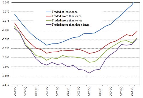
do not change either. The underlying price determination model is basically the same as
in equation (4). However, the repeat sales method focuses on houses that appear multiple
times in the dataset. Suppose that house i is transacted twice, and that the transactions
occur in periods s and t with s < t. Using equations (4), the change in the logarithms of
the house prices between the two time periods is given by

                        ln(Pit /Pis ) = dt − ds − βδ(Aλit − Aλis ) + υit − υis .                        (5)

  Note that the terms that do not include time subscripts in equation (4), namely α ln Li , β ln Bi
and γ · xi , all disappear by taking differences with respect to time, so that the resulting
equation is simpler than the original one.16 Furthermore, assuming no renovation expendi-
tures between the two time periods and no depreciation of housing capital so that δ = 0,
equation (5) reduces to:
                                  ln(Pit /Pis ) = dt − ds + υit − υis .                                 (6)

  The above equation can be rewritten as the following linear regression model:
                                                    ∑T
                                  ln(Pit /Pis ) =           Djits dj + υits                             (7)
                                                      j=1

where υits ≡ υit − υis is a consolidated error term and Djits is a dummy variable that takes
on the value 1 when j = t (where t is the period when house i is resold), the value −1 when
j = s (where s is the period when house i is first sold) and Djits takes on the value 0 for j
not equal to s or t. In order to identify all of the parameters dj , a normalization is required
such as d1 ≡ 0. This normalization will make the house price index equal to unity in the
first period. The standard repeat sales house price indexes are then defined by Pt ≡ exp[d∗t ]
for t = 1, 2, . . . , T , where the d∗t are the least squares estimators for the dt .

2.4     Heteroskedasticity and Age Adjustments to the Repeat Sales
        Index
  As pointed out by previous studies, the standard repeat sales index defined above may be
biased for two reasons:

   • The disturbance term in equation (7) may be heteroskedastic in the sense that the
     variance of the disturbance term may be larger when the two transaction dates are
     further apart.17

   • The assumption of no depreciation is too restrictive.

  Case and Shiller (1987) (1989) address the heteroskedasticity problem in the disturbance
term by assuming that the variance of the residual υits in (7) increases as t and s are
    16 Thus the regression model defined by (5) does not require characteristics information on the house(

except that information on the age of the house at the time of each transaction is required).
    17 However, if s and t are very close, the variance could also increase due to the “flipping phenomenon”;

i.e., a house that is sold twice in a short time period may have a rate of price change between the two time
periods that is unusually large on an annualized basis, causing the error variance to increase.

                                                     6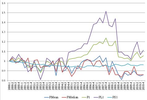
further apart; i.e., they assume that E(υits ) = 0 and E(υits )2 = ξ0 + ξ1 (t − s) where ξ0
and ξ1 are positive parameters. The Case-Shiller repeat sales index is estimated as follows.
First, equation (7) is estimated, and the resulting squared disturbance term is regressed on
ξ0 + ξ1 (t − s) in order to obtain estimates for ξ0 and ξ1 . Denote these estimates by ξ0∗ and ξ1∗ .
Then equation (7) is reestimated by Generalized Least Squares (GLS) where observation i,
ln(Pit /Pis ), is adjusted by the weight [ξ0∗ + ξ1∗ (t − s)]1/2 . Denote the resulting GLS estimates
for the coefficients dt on the time dummy variables by d∗t . The Case-Shiller heteroskedasticity
adjusted repeat sales indexes are then defined by Pt ≡ exp[d∗t ] for t = 1, 2, . . . , T .18
  We turn now to the lack of an age adjustment problem with the repeat sales method.
Previous studies on the repeat sales method, including Bailey, Muth and Nourse (1963) and
Case and Shiller (1987) (1989), do not pay much attention to the possibility that property
characteristics change over time. However, there are no houses that do not depreciate,
implying that the quality of a house at the time of selling depends on its age. Also, the
quality of a house may change over time because of maintenance and renovation. Finally,
its quality may change over time due to changes in the environment surrounding the house,
such as the availability of public transportation, the quality of neighbourhood schools and so
on.19 As far as the Japanese housing market is concerned, the structure of a house typically
depreciates more quickly than in the United States and Europe, which is likely to cause a
larger bias in price indexes if house price depreciation is ignored.
   To take account of the depreciation effect, we go back to equation (5) and rewrite it as
follows:20
                      ln(Pit /Pis ) = dt − ds − βδ[(Ais + t − s)λ − Aλis ] + υits .                          (8)
  Note that repeat sales indexes that do not include an age term (such as the term involving
Ais on the right hand side of the above equation) will suffer from a downward bias.21
  McMillen (2003) considered a simpler version of this model with λ = 1, so that the
depreciation rate is constant over time. When λ = 1, (8) reduces to (9):

                               ln(Pit /Pis ) = dt − ds − βδ(t − s) + υits .                                  (9)

  Note that there is exact collinearity between dt − ds and t − s, so that it is impossible
to obtain estimates for the coefficients on the time dummies. McMillen (2003) measured
the age difference between two consecutive sales in days while using quarterly time dummy
variables, thereby eliminating the exact collinearity between the time dummies and the age
difference.22
  18 As   usual, set d∗1 ≡ d1 ≡ 1 so that P1 ≡ 1.
  19 Note   that the depreciation model defined by (2) can be regarded as a net depreciation model; i.e., it is
depreciation less “normal” renovation and maintenance expenditures. See Diewert (2011) for more on the
topic of constructing a house price index taking depreciation and renovation into consideration.
   20 The analysis which follows is due to Shimizu, Nishimura and Watanabe (2010).
   21 It should be noted that the official S&P/Case-Shiller home price index is adjusted in the following way

to take the age effect into account. Standard & Poor’s (2008: 7) states that “sales pairs are also weighted
based on the time interval between the first and second sales. If a sales pair interval is longer, then it is more
likely that a house may have experienced physical changes. Sales pairs with longer intervals are, therefore,
given less weight than sales pairs with shorter intervals.”
   22 However, one would expect approximate multicollinearity to hold in McMillen’s model so that the

estimated dummy variable parameters may not be too reliable.

                                                       7
Shimizu, Nishimura and Watanabe (2010) eliminated exact multicollinearity by estimating
the nonlinear model defined by (8).23 Once the dt parameters have been estimated by
maximum likelihood or nonlinear least squares (denote the estimates by d∗t with d∗1 set equal
to 0), then the Shimizu, Nishimura and Watanabe repeat sales indexes Pt are defined as
Pt ≡ exp[d∗t ] for t = 1, 2, . . . , T .
  Note that the parameters β and δ are not identified in the nonlinear regression (8) because
they appear only in the form of βδ. This is in sharp contrast with the hedonic regression
model defined by (4), in which β appears not only as a coefficient of the age term but also
as a coefficient on ln Bi , so that β and δ are identified.24

2.5     Rolling Window Hedonic Regressions: Structural Change Ad-
        justments to the Hedonic Index
  Shimizu, Takatsuji, Ono and Nishimura (2010) and Shimizu, Nishimura and Watanabe
(2010) modified the standard hedonic model given by equation (4) so that the parameters
associated with the attributes of a house are allowed to change over time. Structural changes
in the Japanese housing market have two important features. First, they usually occur only
gradually, triggered, with a few exceptions, by changes in regulations by the central and local
governments. Such gradual changes are quite different from “regime changes” discussed by
econometricians such as Bai and Perron (1998) in which structural parameters exhibit a dis-
continuous shift at multiple times. Second, changes in parameters reflect structural changes
at various time frequencies. Specifically, as found by Shimizu, Nishimura and Watanabe
(2010), some changes in parameters are associated with seasonal changes in housing market
activity. For example, the number of transactions is high at the end of a fiscal year, namely,
between January and March, when people move from one place to another due to seasonal
reasons such as job transfers, while the number is low during the summer. One way to
allow for gradual shifts in parameters is to employ an adjacent period regression,25 in which
equation (4) is estimated using only two periods that are adjacent to each other so that
the parameter vector γ in (4) is only held constant for two consecutive periods (as are the
other parameters, α, β, δ and λ). The estimated second period price level, P2 ≡ exp[d∗2 ], is
regarded as a chain type index which is used to update the previously determined index level
for the first period, P1 . This method of index construction allows for gradual taste changes
thereby minimizing the rigidity disadvantage of the pooled regression model defined by (4).
Triplett (2004), based on the presumption that coefficients usually change less between two
adjacent periods than over more extended intervals, argued that the adjacent-period esti-
   23 See Chau, Wong and Yui (2005) for another example where a nonlinear specification of the age effect

was introduced into the hedonic regression in order to eliminate multicollinearity between the age variable
and the time dummy variables.
   24 If the estimated λ parameter for the model defined by (8) turns out to be close to one, then as is

the case for McMillen’s model, there may be an approximate multicollinearity problem with the Shimizu,
Nishimura and Watanabe repeat sales model.
   25 The two period time dummy variable hedonic regression was considered explicitly by Court (1939; 109-

111) as his hedonic suggestion number two. Griliches (1971; 7) coined the term “adjacent year regression”
to describe the two period dummy variable hedonic regression model.

                                                    8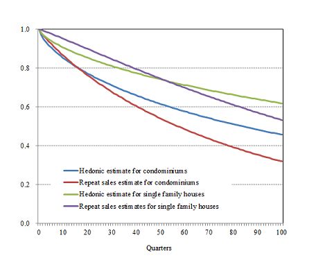
mator is “a more benign constraint on the hedonic coefficients.” However, as far as seasonal
changes in parameters are concerned, this presumption may not necessarily be satisfied,
so that an adjacent period regression may not work very well. To cope with this prob-
lem, Shimizu, Takatsuji, Ono and Nishimura (2010) and Shimizu, Nishimura and Watanabe
(2010) proposed a regression method using multiple “neighborhood periods,” typically 12
or 24 months, rather than two adjacent periods. Specifically, they estimated parameters
by taking a certain length as the estimation window and shifting this period as in rolling
regressions. This method should be able to handle seasonal changes in parameters better
than adjacent period regressions, although it may suffer more from the rigidity disadvantage
associated with pooling.
  To apply this method, estimate the model defined by equations (4) for periods t = 1, . . . , τ ,
where τ < T represents the window width. As usual, set d1 = d∗1 ≡ 1 and denote the
remaining estimated time parameters for this first regression by d∗2 , . . . , d∗τ . These parameters
are exponentiated to define the sequence of house price indexes Pt for the first τ periods; i.e.,
Pt ≡ exp[d∗t ] for t = 1, 2, . . . , τ . Then this τ period regression model using the data for the
periods 2, 3, . . . , τ + 1 can be repeated and a new set of estimated time parameters, d2∗      2 ≡
    2∗           2∗                                               2
1, d3 , . . . , dτ +1 can be obtained. The new price levels Pt for periods 2 to τ +1 can be defined
as Pt2 ≡ exp[d2∗    t ] for t = 2, 3, . . . , τ + 1. Obviously, this process of adding the data of the
next period to the rolling window regression while dropping the data pertaining to the oldest
period in the previous regression can be continued. The focus in the Shimizu, Takatsuji,
Ono and Nishimura (2010) paper was on determining how the structural parameters in (8)
changed as the window of observations changed.26 They did not address the problem of
obtaining a coherent time series of price levels from the multiple estimates of price levels
that result from these overlapping hedonic regressions.
  A coherent strategy for forming a single set of price level estimates from the sequence
of Rolling Window regressions works as follows. As indicated in the previous paragraph,
the sequence of final price levels Pt for the first τ periods is obtained by exponentiating
the estimated time dummy parameters taken from the first Rolling Window regression; i.e.,
Pt ≡ exp[d∗t ] for t = 1, 2, . . . , τ . The next Rolling window regression the data for periods
                                                                                                 2∗
2, 3, . . . , τ + 1 generates the new set of estimated time parameters, d2∗         2∗
                                                                            2 ≡ 1, d3 , . . . , dτ +1
and the new set of price levels Pt2 for periods 2 to τ + 1, defined as Pt2 ≡ exp[d2∗         t ] for
t = 2, 3, . . . , τ + 1. Now use only the last two price levels generated by the new regression to
define the final price level for period τ + 1, Pτ +1 , as the period τ price level generated by the
first regression, Pτ , times (one plus) the rate of change in the price level over the last two
periods using the results of the second regression model; i.e., define Pτ +1 ≡ Pτ (Pτ2+1 /Pτ2 ).
The next step is to repeat the τ period regression model using the data for the periods
                                                                                                        3∗
3, 4, . . . , τ + 2 and obtain a new set of estimated time parameters, d3∗                 3∗
                                                                                   3 ≡ 1, d4 , . . . , dτ +2 .
Define new preliminary price levels Pt3 ≡ exp[d3∗    t ] for t = 3, 4, . . . , τ + 2 and update Pτ +1 by
                         3     3
multiplying it by (Pτ +2 /Pτ +1 ) so that the final price level for period τ +2 is defined as Pτ +2 ≡
Pτ +1 (Pτ3+2 /Pτ3+1 ). Carry on with the same process until PT has been defined. This model
  26 They   called their method the Overlapping Period Hedonic Housing Model (OPHM).

                                                      9
can be called the Rolling Window Hedonic Regression model.27 A major advantage of this
method over the repeat sales model is that as new data become available each period, previous
period index levels are not revised. Note that the Rolling Window Hedonic Regression
method reduces to an adjacent period hedonic regression model if τ equals 2.
    In the following section, the various models defined in this section will be illustrated and
compared using data for Tokyo on both houses and condominiums.

3      A Comparison of Alternative Housing Models for Tokyo
3.1     Data Description
  Section 3 of this paper summarizes the results in Shimizu, Nishimura and Watanabe
(2010), (henceforth referred to as SNW). The data for the SNW paper were collected from
a weekly magazine, Shukan Jutaku Joho (Residential Information Weekly), published by
Recruit Co., Ltd., one of the largest vendors of residential property listings information in
Japan. The Recruit dataset covered the 23 special wards of Tokyo for the period 1986 to
2008, which included the bubble period in the late 1980s and its collapse in the early 1990s.
It contained 157,627 listings for condominiums and 315,791 listings for single family houses,
for 473,418 listings in total.28 Shukan Jutaku Joho provided time series for the price of
an advertised for sale unit from the week it is first posted until the week it is removed.29
SNW used only the price in the final week of listing because that price was close to the final
contract price.30

   27 This is the approach used by Shimizu, Nishimura and Watanabe (2010) to form an overall price in-

dex. Ivancic, Diewert and Fox (2009) recommended a variant of the rolling window model where their
basic hedonic regression model was the Time Product Dummy model which is the application of Summer’s
(1973) Country Product Dummy model to the time series context (from the original application to multi-
lateral comparisons of prices across countries). IDF recommended a (weighted) Rolling Year Time Product
Dummy method where the window length was chosen to be 13 months. For extensions of the IDF model
to more general hedonic regression models, see de Haan and Krsinich (2014). Diewert and Shimizu (2013)
implemented a Rolling Window hedonic regression model for Tokyo houses which will be described later in
section 5. The Rolling Window Hedonic Regression approach to the construction of house price indexes has
also been applied by Eurostat (2011; Chapter 8) and by Diewert, de Haan and Hendriks (2011b).
   28 Shimizu Nishimura and Asami (2004) reported that the Recruit data cover more than 95 percent of all

transactions in the 23 special wards of Tokyo but the coverage for suburban areas is very limited. Therefore
the study by Shimizu, Nishimura and Watanabe used only information for the units located in the special
wards of Tokyo.
   29 There are two reasons for removal of the listing of a unit from the magazine: a successful deal or a

withdrawal; i.e., in the second case, the seller gives up looking for a buyer and thus withdraws the listing.
SNW were allowed to access information regarding which of the two reasons applied for individual cases and
they discarded prices where the seller withdrew the listing.
   30 Recruit Co. Ltd. provided SNW with information on contract prices for about 24 percent of the

population of listings. Using this information, SNW were able to confirm that prices in the final week were
almost always identical to the contract prices; i.e., they differed at less than a 0.1 percent probability.

                                                     10
Table 1. List of variables
Abbreviation Variable Description Unit
GA Ground area Ground area. m2
FS Floor space Floor space of building. m2
RW Front road width Front road width. 10cm
AGE Age of a building at the Age of a building at the time of transaction. Quarters
time of transaction
TS Time to the nearest Time distance to the nearest station (walking Minutes
station time or time by bus or car).
TT Travel time to central Minimum railway riding time in daytime to one Minutes
business district of the seven major business district stations.
UV Unit volume Unit volume/The total number of units of the Unit
condominium.
RT Market reservation Period between the date when the data appear Weeks
time in the magazine for the first time and the date
of being deleted.
BD Bus dummy Time distance to the nearest station includes (0, 1)
taking the bus = 1.; Does not include taking
the bus = 0.
CD Car dummy Time distance to the nearest station includes (0, 1)
taking the car = 1.; Does not include taking
the car = 0.
FD First floor dummy The property is on the ground floor = 1. (0, 1)
The property is not on the ground floor = 0.
BBD Before new building Construction year is before 1980(when New (0, 1)
standard law dummy Building Standard Law enacted)∗ = 1.;
Construction year is after 1981 = 0.
SRC Steel reinforced ”Steel” reinforced concrete frame structure = 1.; (0, 1)
concrete dummy Other structure(Reinforced concrete frame
structure) = 0.
SD South-facing dummy Main windows facing south = 1. (0, 1)
Main windows facing no facing south = 0.
PD Private road dummy Site includes a part of private road∗∗ = 1. (0, 1)
Site does not include any part of private road = 0.
LD Land only dummy The transaction includes ”land” only (no building (0, 1)
is on the site) = 1.;
The transaction includes land and building = 0.
OD Old house dummy∗∗∗ The transaction includes existing buliding which (0, 1)
can not be used = 1.; The transaction doesn’t
include exsitng building which can be used = 0.
BA Balcony area Balcony area. m2
BLR Building-to-land ratio Building-to-land ratio regulated by City Planning %
Law
F AR Floor area ratio Floor area ratio regulated by City Planning Law %
11Abbreviation Variable Description Unit
W Dk Ward dummies Located in ward k = 1.; (0, 1)
Located in other ward = 0. (k = 0, . . . , K)
RDl Railway line dummies Located on railway line l =1.; (0, 1)
Located on other railway line = 0. (l = 0, . . . , L)
T Dm Time dummies Month m = 1.; (0, 1)
(monthly) Other month = 0. (m = 0, . . . , M )
* The new building standard law established earthquake-resistance standards.
** The building standard law prohibits the construction of a building if the site faces a road
which is narrower than 2 meters. If the site does not face a road which is wider than 2 meters,
the site must provide a part of its own site as a part of the road.
*** If there is an existing building which cannot be used, the buyer has to pay the demolition costs.
Table 1 shows a list of the attributes of a house. Key attributes include the ground area
of the land plot (GA), the floor space area of the structure (F S), and the front road width of
the land plot (RW ). The land plot area was available in the original dataset for single family
houses but not for condominiums, so SNW estimated the land area that could be attributed
to a condominium unit by dividing the land area of the property by the number of units in
the structure.31 The age of a detached house was defined as the number of quarters between
the date of the construction of the house and the transaction. SNW constructed a dummy
(south-facing dummy, SD) to indicate whether the windows of a house are south-facing or
not.32 The private road dummy, P D, indicated whether a house had an adjacent private
road or not. The land only dummy, LD, indicated whether a transaction was only for
land without a building or not. The convenience of public transportation from a house was
represented by the travel time to the central business district (CBD),33 which was denoted
by T T , and the time to the nearest station,34 which was denoted by T S. SNW used a
ward dummy, W D, to indicate differences in the quality of public services available in each
district, and a railway line dummy, RD, to indicate along which railway or subway line a
house is located.
SNW used their Tokyo data sets on detached houses and condominiums to construct
housing price indexes that used the hedonic regression and repeat sales models that were
described in section 2 above. Table 2 compares the sample SNW used in their hedonic re-
31 More specifically, the imputed land area attributed to a condo unit was calculated by dividing the sum
of the floor space for each unit in the structure by F AR × BLR, where F AR and BLR stand for the floor
area ratio and the building to land ratio, respectively. The sum of the floor space of each unit in a structure
was available in the original dataset. The maximum values for F AR and BLR are subject to regulation
under city planning law. It was assumed that this regulation was binding.
32 Japanese people are particularly fond of sunshine!
33 Travel time to the CBD was measured as follows. The metropolitan area of Tokyo is composed of wards
and contains a dense railway network. Within this area, SNW chose seven railway or subway stations as
central business district stations: Tokyo, Shinagawa, Shibuya, Shinjuku, Ikebukuro, Ueno, and Otemachi.
SNW then defined travel time to the CBD as the minutes needed to commute to the nearest of the seven
stations in the daytime.
34 The time to the nearest station, T S, was defined as the walking time to the nearest station if a house
was located within walking distance from a station, and the sum of the walking time to a bus stop and the
bus travel time from the bus stop to the nearest station if a house is located in a bus transportation area.
SNW used a bus dummy, BD, to indicate whether a house was located in walking distance from a railway
station or in a bus transportation area.
12gressions and the sample used in their repeat sales regressions. Since repeat sales regressions
use only observations from houses that are traded multiple times, the repeat sales sample is
a subset of the hedonic sample. The ratio of the repeat sales sample to the hedonic sample
is 42.7 percent for condominiums and 6.1 percent for single family houses, indicating that
single family houses are less likely to appear multiple times on the market.
The average price for condominiums was 38 million yen in the hedonic sample, while
it was 44 million yen in the repeat sales sample. On the other hand, the average price
for single family houses was 79 million yen in the hedonic sample and 76 million yen in
the repeat sales sample. Turning to the attributes or characteristics of houses and condos,
houses in the repeat sales sample tended to be larger in terms of the floor space, and more
conveniently located in terms of time to the nearest station and travel time to a central
business district, although these differences are not statistically significant. An important
and statistically significant difference between the two samples was the average age of units
in the case of single family houses: namely, the repeat sales sample consisted of houses
that were constructed relatively recently. Somewhat interestingly, single family houses in
the repeat sales sample were larger in terms of floor space, more conveniently located, more
recently constructed, but were less expensive.
Table 2. Hedonic vs. repeat sales samples
Condominiums Single family houses
Variable Hedonic sample Repeat sales Hedonic sample Repeat sales
sample sample
Average price 3, 862.26 4, 463.43 7, 950.65 7, 635.24
(10,000 yen) (3, 190.83) (4284.10) (8275.04) (7055.96)
F S: Floor space 58.31 59.54 102.53 105.82
(m2 ) (21.47) (24.09) (43.47) (45.60)
GA: Ground area 23.39 20.53 108.20 101.41
(m2 ) (12.79) (11.97) (71.19) (63.17)
Age: Age of building 55.61 60.07 54.06 21.26
(quarters) (33.96) (34.05) (32.28) (30.88)
T S: Time to the 7.96 7.77 9.85 9.60
nearest station (4.43) (4.28) (4.54) (4.37)
(minutes)
T T : Travel time to 12.58 10.73 13.23 11.89
central business district (7.09) (6.88) (6.34) (6.18)
(minutes)
n = 157, 627 n = 67, 436 n = 315, 791 n = 19, 428
133.2 Estimation Results
Table 3 presents the regression results obtained by Shimizu, Nishimura and Watanabe
(2010) for the standard hedonic model given by equation (4). This model worked well, both
for condominiums and single family houses: the adjusted R2 was 0.882 for condominiums
and 0.822 for single family houses. The coefficients of interest are the ones associated with
the age effect. The estimates of δ and λ are 0.033 and 0.691 for condominiums, implying
that the initial capital stock of structures declines to 0.457 after 100 quarters, and that the
average annual geometric depreciation rate for 100 quarters is 0.031. On the other hand, the
estimates of δ and λ for single family houses are 0.020 and 0.688, implying that the initial
capital stock of structures declines to 0.619 after 100 quarters, and that the average annual
depreciation rate for 100 quarters is 0.019. These estimated depreciation rates seem to be
quite reasonable.
Table 4 presents the SNW regression results for the age adjusted repeat sales model given
by equation (8). The estimates for βδ and λ were 0.0098 and 0.894 for condominiums,
and 0.002 and 1.104 for single family houses. Note that the repeat sales regressions do not
allow us to estimate β and δ separately. If estimates of β are borrowed from the hedonic
regressions, the repeat sales regression value of δ turned out to be 0.019 for condominiums
and 0.004 for single family houses. These estimates imply that the average annual rate of
depreciation for 100 quarters is 0.045 for condominiums and 0.025 for single family houses.
Figure 1 compares the hedonic and repeat sales regressions in terms of the estimated age
effect. It can be seen that the estimates from the repeat sales regressions indicate slightly
faster depreciation than the ones from the hedonic regressions both for condominiums and
for single family houses, although the difference is not very large.
Next, turn to the bottom panel of Table 4, which looks at the regression performance
of the three types of repeat sales measures: the standard repeat sales index defined by
equations (6) or (7), the heteroskedasticity adjusted repeat sales index (i.e., the Case-Shiller
index), and the age adjusted repeat sales index defined by (8).35 It can be seen that the age
adjusted repeat sales index performed better than the standard one for both condominiums
and single family houses. On the other hand, SNW failed to find a significant difference
between the age adjusted index and the Case-Shiller index.
35 Note that the estimated coefficient for λ in the age adjusted repeat sales model was 0.89 for condos and
1.10 for single family houses. Thus the exact multicollinearity problem does not arise for these regressions.
14Table 3. Hedonic regressions
Condominiums Single family houses
Variable Coefficient t-value Coefficient t-value
Constant 3.263 372.920 4.508 265.376
GA: Ground area (m2 ) 0.593 21.499 0.548 48.189
T S: Time to the nearest station −0.083 −86.748 −0.118 −129.946
(minutes)
Bus: Bus dummy −0.313 −11.461 −0.079 −2.862
Car: Car Dummy − − −0.408 −6.497
Bus × T S 0.070 6.453 −0.026 −2.580
Car × T S − − 0.068 2.330
T T : Travel time to central −0.041 −30.952 −0.076 −83.494
business district (minutes)
M C: Management cost 0.045 16.135 − −
U V : Unit volume 0.024 33.752 − −
BBD: Before new building −0.085 −126.640 −0.093 −48.965
standard law dummy
SRC: Steel reinforced 0.018 33.620 − −
concrete dummy
BA: Balcony area (m2 ) 0.029 69.850 − −
RW : Road width (10cm) − − 0.190 142.685
P D: Private road dummy − − −0.001 −2.973
LD: Land only dummy − − 0.227 45.634
SD: South facing dummy 0.003 2.203 0.004 1.940
OD: Old house dummy − − −0.103 −56.412
BLR: Building-to-land ratio 0.075 56.572 0.065 18.677
F AR: Floor area ratio 0.039 6.807 0.029 16.347
F S: Floor space (m2 )
β 0.528 20.171 0.487 45.103
Age: Age of building (quarters)
δ 0.033 4.153 0.020 2.423
λ 0.691 98.590 0.688 45.850
n = 714, 506 n = 1, 540, 659
Log likelihood 391552.980 −5138.987
Prob > χ2 = 0.000 0.000
Adjusted R2 = 0.882 0.822
Note : The dependent variable in each case is the log of the price.
15Table 4. Age-adjusted repeat sales regressions
βδ λ
Condominiums
Coef. 0.0098 0.8944
Std. err. 0.0004 0.0113
p-value [.000] [.000]
Single family houses
Coef. 0.0019 1.1041
Std. err. 0.0002 0.0269
p-value [.000] [.000]
Standard error
of reg. Adjusted R2 S.B.I.C.
Condominiums
Standard repeat sales 0.175 0.751 −20311.0
Case-Shiller repeat sales 0.191 0.760 −12925.4
Age-adjusted repeat sales 0.190 0.761 −13246.6
Single family houses
Standard repeat sales 0.211 0.478 −2087.0
Case-Shiller repeat sales 0.218 0.511 −1136.1
Age-adjusted repeat sales 0.218 0.513 −1176.4
S.B.I.C.: Schwarz’s Bayesian information criterion
Figure 1. Estimated depreciation curves
16Following the Rolling Year methodology introduced by Shimizu, Takatsuji, Ono and
Nishimura (2010), Shimizu, Nishimura and Watanabe (2010) estimated the hedonic model
defined by (4) using a window length of 12 months. Their results for the structural param-
eters (averaged over all regressions of window length 12) are presented in Table 5, which
compares key parameters of the standard hedonic model and the corresponding rolling year
hedonic models. For condominiums, it can be seen that the average value of each param-
eter estimated by the rolling hedonic regression was close to the estimate obtained by the
standard hedonic regression. For example, the parameter associated with the floor space
of a house was 0.528 using the standard time dummy hedonic regression model defined by
(4) where the entire sample was used in the single regression, while the average value of
the corresponding parameters estimated by the rolling window regression was 0.517. More
importantly, SNW found that the estimated structural parameters fluctuated considerably
during the sample period. For example, the parameter associated with the floor space of a
house fluctuated between 0.508 and 0.539, indicating that non-negligible structural changes
occurred during the sample period. Similar structural changes occurred for single family
houses.
Table 5. Standard vs. rolling window regressions
Const. FS GA Age TS TT
(βδ) (λ)
Condonimium prices
Standard hedonic model 3.263 0.528 0.593 0.017 0.691 −0.083 −0.041
12-month rolling regression
Average 3.200 0.517 0.608 0.016 0.690 −0.082 −0.042
Standard deviation 0.086 0.079 0.040 0.001 0.035 0.015 0.013
Minimum 2.988 0.508 0.562 0.019 0.654 −0.097 −0.069
Maximum 3.429 0.539 0.613 0.011 0.710 −0.051 −0.025
Single family house prices
Standard hedonic model 4.508 0.487 0.548 0.010 0.688 −0.118 −0.076
12-month rolling regression
Average 4.691 0.485 0.532 0.006 0.681 −0.101 −0.079
Standard deviation 0.176 0.021 0.098 0.001 0.029 0.003 0.002
Minimum 4.496 0.480 0.512 0.007 0.670 −0.110 −0.079
Maximum 4.742 0.495 0.558 0.006 0.700 −0.041 −0.048
Number of models = 265
Note: F S: Floor space
GA: Ground area
Age: Age of building
T S: Time to the nearest station
T T : Travel time to central business district
173.3 Reconciling the Differences between the Five Models
Shimizu, Nishimura and Watanabe (2010) estimated the 5 models explained in section 2
above using their Tokyo data sets for both detached houses and condominiums.36 Figure
2 shows the estimated five indexes for condominiums. The age adjusted repeat sales index
starts in the fourth quarter of 1989, while the other four indexes start in the first quarter of
1986. To make the comparison easier, the indexes are normalized so that they are all equal to
unity in the fourth quarter of 1989. The first thing that can be seen from this Figure is that
there is almost no difference between the standard repeat sales index and the Case-Shiller
repeat sales index. This suggests that heteroskedasticity due to heterogeneous transaction
intervals may not be very important as far as the Japanese housing market is concerned.
Second, the age adjusted repeat sales index behaves differently from the other two repeat
sales indexes. Specifically, it exhibits a less rapid decline in the 1990s, i.e., the period when
the bubble burst. This difference reflects the relative importance of the age effect, implying
that the other two repeat sales indexes, which pay no attention to the age effect, tend
to overestimate the magnitude of the burst of the bubble; i.e., the standard repeat sales
indexes have the predictable downward bias due to their neglect of depreciation. Third,
the two hedonic indexes exhibit a less rapid decline in the 1990s than the standard and the
Case-Shiller repeat sales indexes, and the discrepancy between them tends to increase over
time in the rest of the sample period.37
Figure 3 shows the estimated indexes for single family houses. We see that the three repeat
sales indexes and the standard hedonic index tend to move together, but the rolling hedonic
index behaves differently from them. The spread between the rolling hedonic index and the
other four indexes tends to expand gradually in the latter half of the 1990s, suggesting the
presence of some gradual shifts in the structural parameters during this period.38
36 Their Rolling Window results used a window length of 12 months and used the updating procedure
explained at the end of section 2 above.
37 Note that the age adjusted repeat sales index is well above the other two repeat sales indexes which do
not make an adjustment for depreciation of the structure. This result is to be expected. What is perhaps
more surprising is that the age adjusted repeat sales index ends up well below the two hedonic indexes. This
result may be due to sample selectivity bias in the repeat sales method or to an incorrect specification of
the hedonic models.
38 The annual depreciation rate for houses appears to be much smaller than the corresponding rate for
condos and thus the age bias in the repeat sales models will be much smaller for houses than for condos. The
relatively large differences in the two hedonic indexes is a bit of a puzzle. Diewert and Shimizu (2013) also
compared Rolling Window house price indexes with a corresponding index based on a single time dummy
regression and did not find large differences (but the sample period was much shorter in the Diewert and
Shimizu study).
18Figure 2. Estimated five indices for condominiums
Figure 3. Estimated five indices for single family houses
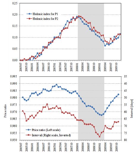
19Figure 4. Comparison of the five indexes in terms of the quarterly growth rate
SNW compared the five indexes for condominiums in terms of their quarterly growth rates.
The results are presented in Figure 4. The horizontal axis in the upper left panel represents
the growth rate of the standard repeat sales index, while the vertical axis represents the
growth rate of the Case-Shiller repeat sales index. One can clearly see that almost all dots
in this panel are exactly on the 45 degree line, implying that these two indexes are closely
correlated with each other. In fact, the coefficient of correlation is 0.995 at the quarterly
frequency, and 0.974 at the monthly frequency. Regressing the quarterly growth rate of
the Case-Shiller repeat sales index, denoted by y, on that of the standard repeat sales
index, denoted by x, SNW obtained y = 0.9439x − 0.0002, indicating that the coefficient
on x and the constant term are very close to unity and zero, respectively. Similarly, the
lower left panel of Figure 4 compares the growth rate of the standard repeat sales index
and the age-adjusted repeat sales index. Again, almost all dots are on the 45 degree line,
indicating a high correlation between the two indexes (the coefficient of correlation is 0.991
at the quarterly frequency and 0.953 at the monthly frequency). However, the regression
results show that the constant term is slightly above zero, indicating that the growth rates
for the age adjusted repeat sales index are, on average, slightly higher than those for the
standard repeat sales index. Turning to the upper right panel, which compares the standard
hedonic index and the standard repeat sales index, the dots are again scattered along the
2045 degree line but not exactly on it, indicating a lower correlation than before (0.845 at the
quarterly frequency and 0.458 at the monthly frequency). More importantly, SNW obtained
y = 1.0948x + 0.0036 by regressing the standard hedonic index on the standard repeat sales
index, and the constant term turned out to be positive and significantly different from zero.
In other words, the standard hedonic index tends to grow faster than the standard repeat
sales index, which is consistent with what is seen in Figure 2.39 Finally, the lower right
panel compares the standard repeat sales index and the rolling hedonic index, showing that
the two indexes are more weakly correlated (0.773 at the quarterly frequency and 0.444 at
the monthly frequency), and that the rolling hedonic index tends to grow faster than the
standard repeat sales index.
SNW also regressed the quarterly growth rate of one of the five indexes, say index A, on the
quarterly growth rate of another index, say index B, to obtain a simple linear relationship
y = a + bx. They then conducted an F -test against the null hypothesis that a = 0 and
b = 1. The results of this exercise are presented in Table 6, where the number in each
cell represents the p-value associated with the null hypothesis that a = 0 and b = 1 in a
regression in which the index in the corresponding row is the dependent variable while the
index in the corresponding column is the independent variable. For example, the number
in the lower left corner of the upper panel, 0.0221, represents the p-value associated with
the null hypothesis in the regression in which the growth rate of the rolling hedonic index
is the dependent variable and the growth rate of the standard repeat sales index is the
independent variable. The upper panel, which presents the results for condominiums, shows
that in almost all cases the null hypothesis cannot be rejected. However, there are two cases
in which the p-value exceeds 10 percent: when the standard hedonic index is regressed on
the age adjusted repeat sales index (p-value = 0.2120), and when the rolling hedonic index
is regressed on the standard hedonic index (p-value = 0.1208). Looking at the lower panel of
Table 6, which presents the results for single family houses, we see that there are more cases
in which the null hypothesis is rejected. For example, the p-value is very high at 0.7661
when the standard hedonic index is regressed on the standard repeat sales index, so that
the null hypothesis that the hedonic and the repeat sales indexes are close to each other can
easily be rejected.
39 It can be seen from the upper right panel of Figure 4 that several dots in the right upper quadrant are
well above the 45 degree line, indicating that the growth rates of the standard hedonic index are substantially
higher than those of the standard repeat sales index at least for these quarters. These dots correspond to
the quarters between 1986 and 1987, during which the standard hedonic index exhibited much more rapid
growth than the standard repeat sales index, as was seen in Figure 2.
21You can also read