Adverse Weather Scenarios for Future Electricity Systems: Developing the dataset of long-duration events
←
→
Page content transcription
If your browser does not render page correctly, please read the page content below
Adverse Weather Scenarios for Future
Electricity Systems: Developing the
dataset of long-duration events

June 24, 2021
Authors: Dr Laura Dawkins, Isabel Rushby and Megan Pearce
Expert guidance from: Dr Theodoros Economou, Dr Simon Brown,
Dr Jason Lowe and the project advisory group
Reviewed by: Tom Butcher, Dr Simon Brown and Dr Emily Wallace

  www.metoffice.gov.uk                   c Crown Copyright 2021, Met Office
Disclaimer
  • This document is published by the Met Office on behalf of the Secretary of State for Business,
    Energy and Industrial Strategy, HM Government, UK. Its content is covered by c Crown Copyright
    2021.
  • This document is published specifically for the readership and use of National Infrastructure Com-
    mission and may not be used or relied upon by any third party, without the Met Office’s express
    written permission.

  • The Met Office aims to ensure that the content of this document is accurate and consistent with
    its best current scientific understanding. However, the science which underlies meteorological
    forecasts and climate projections is constantly evolving. Therefore, any element of the content of
    this document which involves a forecast or a prediction should be regarded as our best possible
    guidance, but should not be relied upon as if it were a statement of fact. To the fullest extent
    permitted by applicable law, the Met Office excludes all warranties or representations (express or
    implied) in respect of the content of this document.
  • Use of the content of this document is entirely at the reader’s own risk. The Met Office makes no
    warranty, representation or guarantee that the content of this document is error free or fit for your
    intended use.
  • Before taking action based on the content of this document, the reader should evaluate it thor-
    oughly in the context of his/her specific requirements and intended applications.
  • To the fullest extent permitted by applicable law, the Met Office, its employees, contractors or
    subcontractors, hereby disclaim any and all liability for loss, injury or damage (direct, indirect,
    consequential, incidental or special) arising out of or in connection with the use of the content of
    this document including without limitation any and all liability:

       – relating to the accuracy, completeness, reliability, availability, suitability, quality, ownership,
         non-infringement, operation, merchantability and fitness for purpose of the content of this
         document;
       – relating to its work procuring, compiling, interpreting, editing, reporting and publishing the
         content of this document; and
       – resulting from reliance upon, operation of, use of or actions or decisions made on the basis
         of, any facts, opinions, ideas, instructions, methods, or procedures set out in this document.

  • This does not affect the Met Office’s liability for death or personal injury arising from the Met
    Office’s negligence, nor the Met Office’s liability for fraud or fraudulent misrepresentation, nor any
    other liability which cannot be excluded or limited under applicable law.
  • If any of these provisions or part provisions are, for any reason, held to be unenforceable, illegal
    or invalid, that unenforceability, illegality or invalidity will not affect any other provisions or part
    provisions which will continue in full force and effect.

c Crown Copyright 2021, Met Office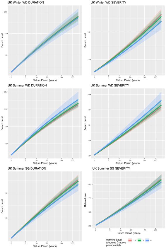
Contents
Contents 1
1 Executive Summary 3
2 Introduction 5
3 Summary of Phase 2 (a): Characterising long-duration adverse weather events 7
3.1 Estimating Weather Dependent Electricity Demand . . . . . . . . . . . . . . . . . . . . . . 7
3.2 Estimating Wind Electricity Generation . . . . . . . . . . . . . . . . . . . . . . . . . . . . . 8
3.3 Estimating Solar Electricity Generation . . . . . . . . . . . . . . . . . . . . . . . . . . . . . 9
3.4 The Wind-Drought-Peak-Demand Index (WDI) . . . . . . . . . . . . . . . . . . . . . . . . 9
3.5 The Surplus-Generation-Index (SGI) . . . . . . . . . . . . . . . . . . . . . . . . . . . . . . 10
3.6 Sensitivity Study . . . . . . . . . . . . . . . . . . . . . . . . . . . . . . . . . . . . . . . . . 13
4 Developing the dataset of long-duration adverse weather scenarios for future electricity
systems 14
4.1 Data sources . . . . . . . . . . . . . . . . . . . . . . . . . . . . . . . . . . . . . . . . . . . 15
4.1.1 DePreSys Hindcasts . . . . . . . . . . . . . . . . . . . . . . . . . . . . . . . . . . . 15
4.1.2 UK Climate Projections 2018 (UKCP18) . . . . . . . . . . . . . . . . . . . . . . . . 16
4.2 Data calibration . . . . . . . . . . . . . . . . . . . . . . . . . . . . . . . . . . . . . . . . . . 16
4.2.1 Bias correction of 10m wind speed, surface temperature and mean sea level pres-
sure . . . . . . . . . . . . . . . . . . . . . . . . . . . . . . . . . . . . . . . . . . . . 17
4.2.2 Representing 100m wind speed . . . . . . . . . . . . . . . . . . . . . . . . . . . . 21
4.2.3 Representing surface solar radiation . . . . . . . . . . . . . . . . . . . . . . . . . . 25
4.2.4 Spatio-temporal statistical downscaling . . . . . . . . . . . . . . . . . . . . . . . . 29
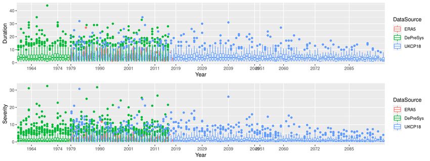
4.3 Exploring adverse weather scenarios in ERA5, DePreSys and UKCP18 . . . . . . . . . . 31
4.4 Statistical extreme value analysis to quantify adverse weather in different climates . . . . 41
4.5 Selecting adverse weather scenarios for the final dataset . . . . . . . . . . . . . . . . . . 52
5 The Adverse Weather Scenarios for Future Electricity Systems dataset 56
5.1 Downloading the data . . . . . . . . . . . . . . . . . . . . . . . . . . . . . . . . . . . . . . 57
6 Summary and Conclusion 60
7 References 63
8 Glossary 66
c Crown Copyright 2021, Met Office 1 of 85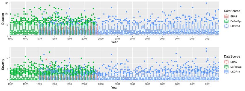
A Appendix                                                                                             67
  A.1 Validation of Calibrated DePreSys data . . . . . . . . . . . . . . . . . . . . . . . . . . . . 67
  A.2 Tables of selected events . . . . . . . . . . . . . . . . . . . . . . . . . . . . . . . . . . . . 74
  A.3 Data download README file . . . . . . . . . . . . . . . . . . . . . . . . . . . . . . . . . . 82

c Crown Copyright 2021, Met Office                                                                2 of 85
1 Executive Summary
The first National Infrastructure Assessment (National Infrastructure Commission, 2018), published by
the National Infrastructure Commission (the Commission) in 2018, recommends targeting a transition
of the UK electricity system to a highly renewable generation mix, incorporating increasing wind and
solar power capacities. This is consistent with a number of other recent reports such as the Climate
Change Committee’s Sixth Carbon Budget report (Climate Change Committee, 2020), and the Interna-
tional Energy Agency’s Net Zero by 2050 Roadmap for the Global Energy Sector (International Energy
Agency, 2021), all reflecting the need for a de-carbonised energy system to help tackle the climate crisis.
Whilst desirable, transitioning to this highly renewable mix will increase the vulnerability of the UK’s
electricity system to adverse weather conditions, such as sustained periods of low wind speeds lead-
ing to low wind generation, coupled with cold winter or high summer temperatures leading to peak
electricity demand. Consequently, the Commission want to improve understanding of the impact of ad-
verse weather conditions on a highly-renewable future system. This will support the recommendations
it makes to government and provide beneficial inputs to those that model and design future electricity
systems.
To improve this understanding, the Met Office have been working with the National Infrastructure Com-
mission and Climate Change Committee to develop a dataset of adverse weather scenarios, based
on physically plausible weather conditions, representing a range of possible extreme events, and the
effect of future climate change. This dataset will allow for proposed future highly renewable electricity
systems to be stress tested to evaluate resilience to challenging weather and climate conditions. This
insight comes at a relevant time - as reported in the Drax quarterly Energy Insights report (Staffell et al.,
2021), the start of 2021 saw unusually cold weather coupled with plant outages, creating very tight
supply margins, highlighting the need for intelligent future planning.
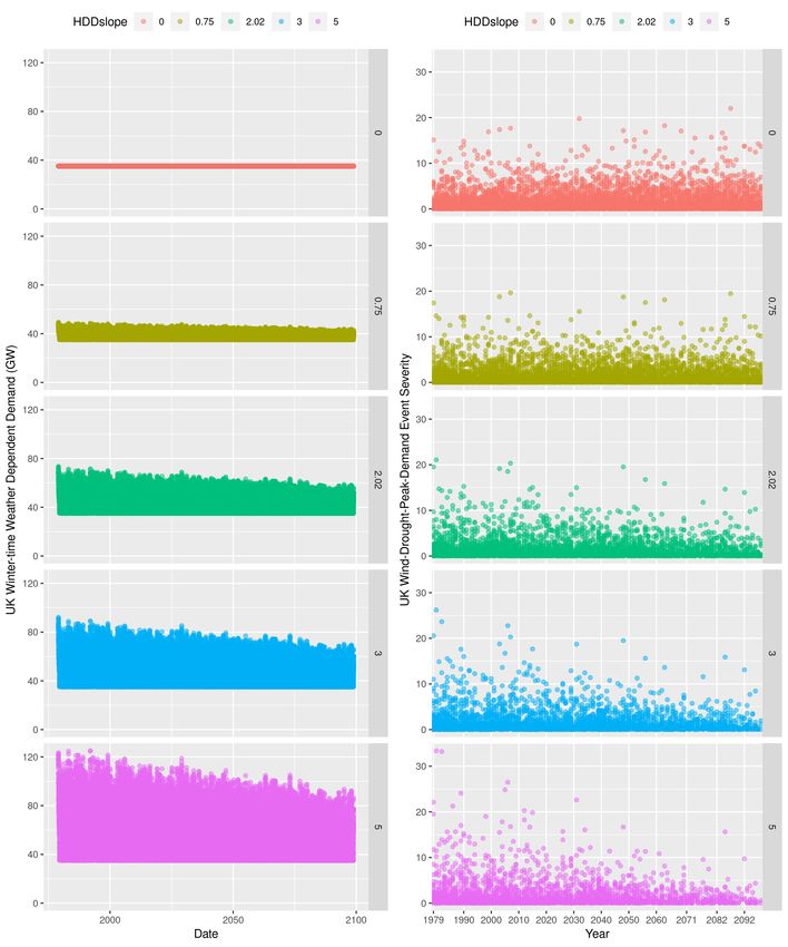
This report presents the development of this dataset of long-duration adverse weather scenarios. This
dataset characterises winter-time and summer-time wind-drought-peak-demand events, and summer-
time surplus generation events, in the UK and in Europe. It contains gridded daily average meteo-
rological data (surface temperature, 100m wind speed and surface solar radiation) associated with a
range of examples of such events, capturing various extreme levels (1 in 2, 5, 10, 20, 50 and 100 year
return period events) and climate warming levels (current day, 1.5◦ C, 2◦ C, 3◦ C and 4◦ C above pre-
industrial levels). The dataset is freely available to download from the Centre for Environmental Data
Analysis archive1 , and a brief how-to guide for downloading the data is included at the end of this report.
Firstly, a summary of the methods developed for characterising and identifying long-duration adverse
1 https://catalogue.ceda.ac.uk/uuid/7beeed0bc7fa41feb10be22ee9d10f00 (Accessed 01/06/2021)
c Crown Copyright 2021, Met Office 3 of 85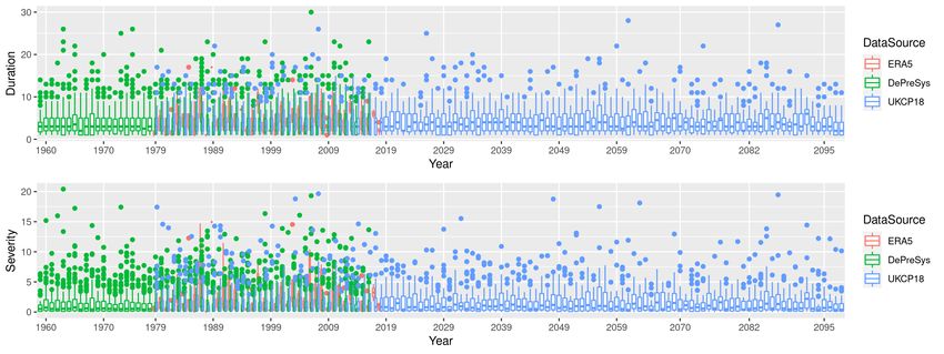
weather events within any suitable gridded meteorological dataset, is given. These methods are based
on insights from the energy modelling literature, and aim to be as energy system agnostic as possi-
ble. The approach taken for developing the final dataset is then presented. Adverse weather scenarios
are identified in three data sources: historical observations; historical climate model hindcasts (provid-
ing more than 2000 alternative plausible weather years) and future climate projections (capturing how
weather is likely to change in future climates). The methods developed for calibrating and imputing
these climate model data sources are presented. These steps are necessary to ensure the data is fit
for purpose.

Adverse weather scenarios identified across these three data sources are then used in combination
to quantify the extremity (i.e. the return period) of events, and how these may change in future warmer
climates. This information is subsequently used to select relevant events for the final dataset. The
sensitivity of the highly-renewable UK electricity system to climate change (particularly rising global
temperatures) is explored and discussed. This highlights how, in a UK system with high wind and solar
renewable capacity, changing the generation or demand assumptions would not materially change the
events identified as adverse, except where extreme levels of electric air conditioning for heating and
cooling are tested.

This study therefore provides a consistent approach for identifying, characterising and quantifying ad-
verse weather scenarios for highly-renewable electricity systems, while aiming to be as energy system
agnostic as possible. The resulting ‘Adverse Weather Scenarios for Future Electricity Systems’ dataset
of long-duration events is therefore relevant for stress testing a range of potential future electricity sys-
tems, ultimately helping to ensure security of supply in a future net-zero world.

c Crown Copyright 2021, Met Office                                                                   4 of 85
2        Introduction

The Met Office has developed a dataset of adverse weather events that can be used by energy sys-
tem modellers to test the weather and climate resilience of potential future highly renewable electricity
systems. Following on for the initial literature review (Dawkins, 2019), project scoping report (Butcher
and Dawkins, 2020), and the characterisation of long-duration adverse weather stress events (Dawkins
and Rushby, 2021), this report presents the development of the ‘Adverse Weather Scenarios for Future
Electricity Systems’ dataset of long-duration events.

As described in (Butcher and Dawkins, 2020), the final dataset is required to represent three forms
of long-duration adverse weather scenario: winter-time wind-drought-peak-demand events, summer-
time wind-drought-peak-demand events, and summer-time surplus generation events. These events
are required to be contained within whole years of gridded meteorological data, for different regions (UK
and Europe), at various extreme levels (1 in 2, 5, 10, 20, 50 and 100 year return period events), and for
different climate warming levels (current day, 1.5◦ C, 2◦ C, 3◦ C and 4◦ C above pre-industrial levels).

Basing this adverse weather dataset on the historical observed record only, i.e. the ERA5 reanaly-
sis data set (Hersbach et al., 2018), may only capture a narrow range of plausible weather conditions,
and will not represent how such events may change in future climates. Therefore, methods previously
developed for characterising and identifying long-duration adverse weather scenarios (Dawkins and
Rushby, 2021), are applied to two additional data sources. Namely, the Met Office Decadal Predic-
tion System (DePreSys)2 hindcast (Dunstone et al., 2016), providing 40 alternative realisation of the
historical period 1959-2016, and hence additional plausible weather conditions, and the UK Climate
Projections (UKCP18) (Lowe et al., 2018), representing how weather is likely to change in the future
as a result of climate change. The adverse weather scenarios identified in these three data sources
are used in combination within a non-stationary statistical extreme value analysis (EVA) to quantify the
likelihood (i.e. the return period) of events, and how these may change in future warmer climates. The
results of this analysis are then used to pick relevant adverse weather scenarios from the DePreSys
and UKCP18 datasets, to be used to represent the various required extreme levels and warming levels
within the final dataset.

The DePreSys and UKCP18 data sources are both derived from climate models, hence methods are
developed for validating, calibrating and imputing the data where necessary. This ensures, for example,
that the climate model data is not too hot or too windy on average. Specifically, a univariate variance
scaling approach is used to bias correct the model data, and data science generalised additive models
are developed to estimate 100m (above ground) wind speed from 10m wind speed, and to estimate
surface solar radiation coherently with other DePreSys weather variables. In addition, in both cases the
    2A   glossary of acronyms is presented in Section 8

c Crown Copyright 2021, Met Office                                                                   5 of 85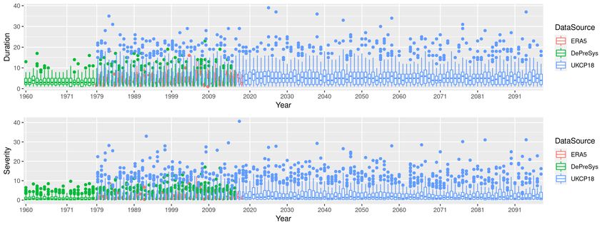
climate model data is available on a 60 km × 60 km, daily spatial-temporal resolution, hence methods
for downscaling in space and time are explored.

This report firstly summaries the approach developed for characterising long-duration adverse weather
scenarios, as previously published in Dawkins and Rushby (2021). The method for creating the final
dataset of long-duration adverse weather scenarios for future electricity systems is then presented.
Initially, the two climate model datasets (DePreSys and UKCP18) are introduced, and the methods for
calibrating and imputing them are described. The adverse weather scenarios identified in the three data
sources are then compared and explored. Following this, the statistical EVA method used to quantify
the likelihood of adverse weather scenarios in different climates is presented, and the approach used
to select relevant periods of adverse weather for the final dataset, based on this analysis, is given. Fi-
nally, a full specification of the final ‘Adverse Weather for Future Electricity Systems’ dataset is provided,
along with a brief how-to guide on how to download the dataset from the Centre for Environmental Data
Analysis (CEDA) archive.

c Crown Copyright 2021, Met Office                                                                    6 of 85
3        Summary of Phase 2 (a): Characterising long-duration adverse
         weather events

The Phase 2 (a) report (Dawkins and Rushby, 2021) presents the development and validation of an ap-
proach for characterising adverse weather events using meteorological data, focusing on long-duration
wind-drought-peak-demand and surplus generation events. This method was applied to 40 years of his-
torical (1979-2018) meteorological data taken from the ERA5 meteorological reanalysis dataset (Hers-
bach et al., 2018), and the resulting adverse weather events within the historical report were presented.

Since these adverse weather events occur when electricity generation and demand are high or low,
methods for estimating electricity generation and demand from weather data were first developed.
These representations of electricity generation and demand were then used to quantify unfavourable
conditions through adverse weather metrics. In doing so, this approach draws on insights from the elec-
tricity modelling literature, such as Bloomfield et al. (2019), hydrological drought modelling literature,
such as Burke et al. (2010), and the expertise of the project advisory and user groups.

The following section provides a brief summary of the Phase 2 (a) approach to give context for the
application of these methods in Phase 2 (b), as presented in Sections 4 and 5. Please refer back to the
Phase 2 (a) report for further detail (Dawkins and Rushby, 2021).

3.1       Estimating Weather Dependent Electricity Demand

Weather dependent demand (WDD)3 is estimated from 2m above group (surface) air temperature data
using the same method as developed by Bloomfield et al. (2019) (documented in their supplementary
material). The relationship between temperature and weather dependent demand is modelled as being
linear, with a different gradient below and above certain thresholds, representing the increase in heating
or cooling demand with temperature. This is implemented using the following metrics:

    1. Heating degree days (HDD): When regional daily average temperature is below the chosen heat-
         ing threshold (15.5◦ C), HDD is equal to the heating threshold minus the temperature on that day,
         and zero otherwise.

    2. Cooling degree days (CDD): When regional daily average temperature is above the chosen cooling
         threshold (22.0◦ C), CDD is equal to the temperature on that day minus the cooling threshold, and
         zero otherwise.

The WDD in a given country is then calculated as a function of the regional baseline electricity demand,
HDD and CDD. These three parameters are different for each country, as presented in the supplemen-
tary material of Bloomfield et al. (2019) and in Table 10 of Dawkins and Rushby (2021).
    3A   glossary of acronyms is presented in Section 8

c Crown Copyright 2021, Met Office                                                                 7 of 85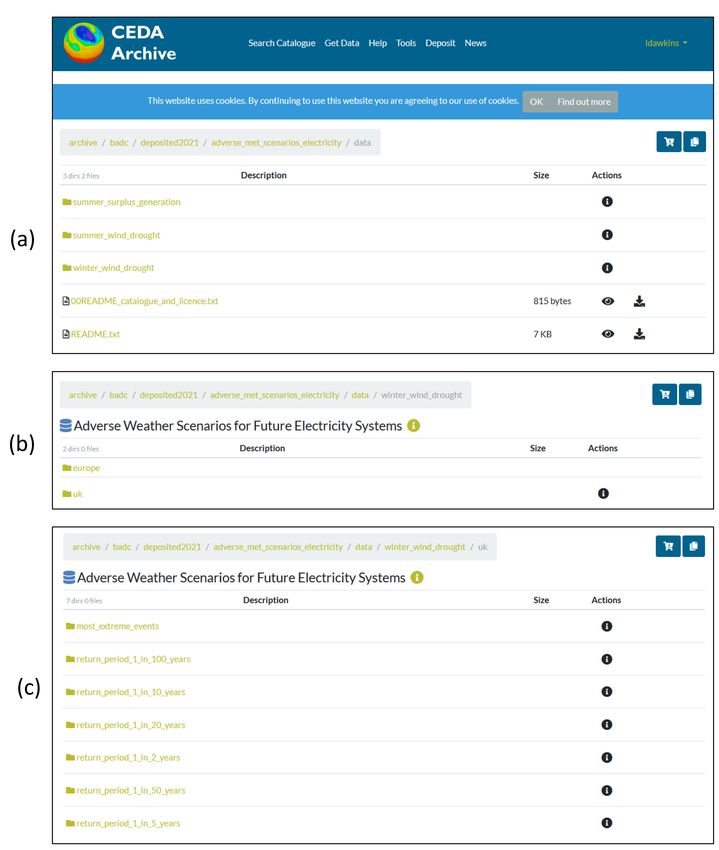
As described in (Butcher and Dawkins, 2020), the latest UK climate projections released by the Met
Office in November 2018 (Lowe et al., 2018) show a clear increasing signal in UK temperatures. In
particular, summer maximum temperatures are on average likely to rise by 2-3◦ C in the south of the
UK by 2100. Indeed, Sanderson et al. (2016) show how, by the mid-21st century, southern and central
England and Wales are likely to have climates analogous to the current climate of northern and western
France. This change in the future UK climate is likely to change cooling demand within the UK, with
more people using air conditioning to improve their comfort during the hotter summers. For this reason,
in this study, the UK demand model of Bloomfield et al. (2019) is modified to incorporate the cooling
slope of the French model (taken to be an analogue for the UKs future climate). This is done to ensure
that the increased demand for cooling in the UK, as a result of the rising summer-time temperatures, is
captured when applying the method to future climate projections (See section 4.3).

3.2      Estimating Wind Electricity Generation

Regional daily wind renewable electricity generation is calculated using 100m wind speed data, to rep-
resent wind speed at turbine hub height. As in Bloomfield et al. (2019), the ERA5 100m wind speed
data is bias corrected in each grid cell using the Global Wind Atlas4 . For a given grid cell and day, the
wind capacity factor, defined as the proportion of a turbines maximum possible generation, is calculated
by applying a turbine power curve to the daily average wind speed in that grid cell. Here, the same 3
turbine power curves as presented in Bloomfield et al. (2019) are used. These represent the type 1, 2
and 3 turbines from the International Electrotechnical Commission (IEC) wind speed classification (IEC,
2005).

In each land grid cell, the most appropriate turbine (of these three options) is chosen. As in Bloom-
field et al. (2019), the selected turbine type is the one that maximises the wind capacity factor for the
40-year (1979-2018) mean of the bias corrected 100m wind speed in that grid cell, and it is assumed
that all of the turbines within a given grid cell are of the same type. The wind power capacity factor is
then weighted by the installed wind capacity within the grid cell (as a fraction of the national total) and
then aggregated over a region/country. The potential for installed wind capacity within each grid cell in
Great Britain is based on technical, social and environmental restrictions explored by Price et al. (2018),
Moore et al. (2018) and Price et al. (2020), with a more simplistic approach across the rest of Europe
(turbines could be located anywhere onshore other than urban areas).

Finally, for a given day, the regional total wind generation is calculated by multiplying the daily regional
capacity factor by the national level of installed wind power. The current day national level of installed
wind power in each country can be obtained from the thewindpower.net website. Since this study is
concerned with capturing adverse weather events for a highly-renewable electricity system, the current
  4 https://globalwindatalas.info   (Accessed 29/04/2021)

c Crown Copyright 2021, Met Office                                                                  8 of 85
day national levels of installed wind power are scaled up to represent a plausible highly-renewable future
as of 2050. Specifically, a national installed capacity of 120GW is employed for the UK and 600GW for
Europe as a whole (with the proportion of European installed capacity in each country consistent with
current day).

3.3     Estimating Solar Electricity Generation

Regional daily solar generation is calculated from surface air temperature and incoming surface solar
radiation. Firstly, on a given day and within a given land grid cell, the solar power capacity factor, defined
as the proportion of a solar panels maximum possible generation produced, is calculated based on a
linear function of the surface temperature and incoming surface solar radiation, as in Bett and Thornton
(2016). Similar to the wind generation calculation, the solar capacity factor is then weighted by the
installed solar capacity within that grid cell (as a fraction of the national total). Within each grid cell, this
installed solar capacity is based on the potential location of solar renewables, as defined by Price et al.
(2018) for Great Britain, and using a simplistic approach of a uniform distribution for the rest of Europe
(i.e. it is assumed that solar renewables can be installed anywhere, as in Bloomfield et al. (2019)).

Finally, for a given day, the regional total solar generation is calculated by multiplying the daily regional
capacity factor by the national level of installed solar renewables. The current day national level of in-
stalled solar in each country can be obtained from the National Generation Capacity Data Platform5 .
Similar to the wind generation calculation, a plausible highly-renewable future as of 2050 is represented
here, by employing a national installed capacity of 100GW in the UK, and 800GW for Europe as a whole
(again such that the proportion of European installed capacity in each country is consistent with current
day).

3.4     The Wind-Drought-Peak-Demand Index (WDI)

The method for calculating the WDI is shown in the schematic in Figure 1.The estimates of daily weather
dependent demand (Section 3.1) and daily wind generation (Section 3.2) are used to calculate daily
Demand-Net-of-Renewables (DNR) for each county, defined as daily weather dependent demand mi-
nus wind generation. This DNR metric therefore represents how much of the daily demand must be
met by energy sources other than wind renewables. Hence, in a highly renewable electricity system,
stressful meteorological days will be associated with positive values of this metric, and adverse weather
events will be associated with periods of time when this metric is particularly high.

Borrowing insights from hydrological drought modelling (Burke et al., 2010), in which drought is char-
acterised by accumulating rainfall over several months, here the DNR metric is accumulated over every
7 day period, representing how ‘bad the previous week has been in terms of weather dependent DNR.
  5 https://data.open-power-system-data.org/national_generation_capacity/    (Accessed 13/01/2021)

c Crown Copyright 2021, Met Office                                                                       9 of 85
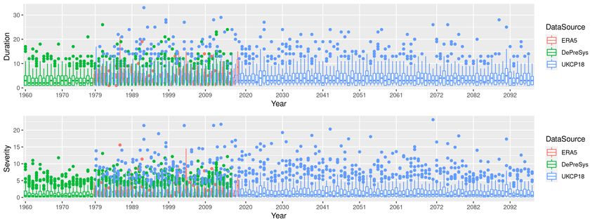
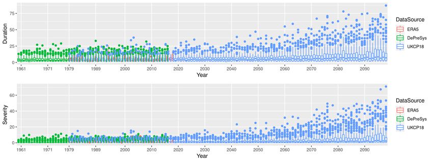
This is then scaled by its long-term average and standard deviation to give the final WDI.

The WDI is used to identify periods of adverse weather, based on when the WDI exceeds a high thresh-
old. These ‘events can then be quantified in terms of duration and severity, and particular events related
to relevant return periods (e.g. 1 in 20 year event) in terms of their duration and severity can be identified.
The duration is the number of days over which the WDI exceeds the adverse weather threshold, and the
severity is the accumulated difference between the WDI and the threshold over the duration of the event.

A different threshold is used in winter (October - March) and summer (April - September). Specifi-
cally, the threshold is defined as the 90th percentile of summer-time WDI in the summer (over the 40
historical years of data), and equivalently the 90th percentile of winter-time WDI in the winter. This
means that 10% of summer days and 10% of winter days within the period of interest will be classed as
adverse, ensuring that an equal proportion of events occur in each season.

3.5    The Surplus-Generation-Index (SGI)

The method for calculating the SGI is shown in the schematic in Figure 2. Daily weather dependent
demand (Section 3.1), daily wind generation (Section 3.2), and daily solar generation (Section 3.3) are
used together to calculate daily Renewables-Net-of-Demand (RND), defined as wind generation plus
solar generation, minus weather dependent demand. This allows the characterisation of surplus gen-
eration adverse weather events via the SGI. These events occur within a region when wind speed and
solar radiation are high, leading to high renewable electricity generation; and temperatures are moder-
ate to high/low, leading to low heating/cooling demand in winter/summer. This form of adverse weather
event is explored in the summer time only (as specified in the scoping phase of this project Butcher and
Dawkins 2020).

Similar to the WDI, the SGI is based on the difference between generation and demand (here RND)
accumulated over every 7-day period (scaled by its long-term average and standard deviation), repre-
senting how bad the previous week has been in terms of accumulating surplus renewable generation
net of weather dependent demand. Again, this metric is used to identify periods of adverse weather
based on exceedance of its 90th percentile. While summer-time (April-September) surplus generation
events are the main focus of this analysis, the SGI is calculated for the whole year, using a different
seasonal threshold (as in the WDI), so that events that start in summer months but continue on into the
winter can be fully captured. These identified surplus generation events can then be quantified in terms
of duration and severity and particular events related to relevant return periods (e.g. 1 in 20 year event)
can be identified.

As these events are based on both wind and solar generation, the relative contribution of each form
of generation to the overall accumulated surplus generation (i.e. the SGI) is also quantified. This metric

c Crown Copyright 2021, Met Office                                                                    10 of 85
Regional Daily Weather Dependent Demand
                     1. For each day, calculate average
                                                                   2. Use the
                     temperature over land in the                                                    Regional demand
                                                                   national demand                   on that day
                     region (e.g. UK), using gridded
                                                                   model to
                     temperature data (e.g. ERA5)
                                                                   calculate
                                                                   weather
                                                                   dependent
                                                                   demand
                                                                   associated with                               Regional
                                                                                                                 average
                                                                   that temperature                              temperature on
                                                                                                                 a given day
                                                                   (e.g. 50GW)

                                                                                                                                       3. Repeat
                                                                                                                                       for each
                                                                                                                                       day (e.g.
                                                       Temp                                                                            winter
                                                       (oC)
                                                                                                                                       2010/11)

                  Regional Daily Wind Generation
                      1. Bias correct 100m gridded wind                                                                                Turbine
                      speed data (e.g. ERA5)                                                             Associated                     power
                                                                                       Wind              grid cell
                                                                                                         capacity
                                                                                                                                         curve
                                                                                      speed              factor on
                                                                                      in one             that day

                                                                                       grid                           Grid cell wind
                                                                                        cell                          speed on a
                                                                                                                      given day

                                                                                    2. For each grid cell in the region (e.g. UK),
                                                                                    and each day, calculate the wind capacity
                                                                                    factor using the assign wind turbine power
                                                                                    curve in that grid cell
                                                              100m wind
                                                              speed (m/s)         4. Repeat for each day (e.g. winter 2010/11)

                    3. To calculate regional daily wind generation,
                    multiply the wind capacity factor in each grid cell
                    by the grid cell installed wind capacity weighting,
                    aggregate over the whole region, and multiply by
                    the regional total installed wind capacity

                  The Wind-Drought-Peak-Demand Index
                    1. For the region of interest (e.g. UK),
                    calculate Demand Net of Renewables as
                    demand minus wind generation on each day

                    2. Calculate the 7-day accumulated demand
                    net of renewables by aggregating over each
                    7 day period

                    3. Calculate the Wind-Drought-Peak-
                    Demand index by scaling the 7-day
                    accumulated demand net of renewables by
                    its long-term average and standard                      90th percentile of WDI            Event severity (shaded area)
                    deviation. Identify events as times when the                                       Event
                    index exceeds its 90th percentile, and                                            duration
                    calculate event durations and severities

Figure 1: A schematic demonstrating the step-by-step methods used to (top panel) calculate regional daily weather dependent demand, (middle
panel) calculate regional daily wind renewable electricity generation, and (bottom panel) calculate the wind-drought-peak-demand event index,
identify adverse weather events, and calculate their duration and severity.

c Crown Copyright 2021, Met Office                                                                                                                 11 of 85
can be used to help identify events of interest within the final dataset e.g. those that are more associated
with wind or solar generation.
Regional Daily Solar Generation Surface temperature and solar
radiation in one grid cell
1. Calculate daily average incoming
solar radiation and surface
temperature for land grid cells over
a region (e.g. from ERA5)
Grid cell solar
radiation on a
given day
2. For each grid cell in the region (e.g. UK), and
each day, calculate the solar capacity factor
from solar radiation and temperature using
the solar model of Bloomfield et al. (2019)
Temp
(oC) Solar radiation
(kWh/m2)
4. Repeat for each day (e.g. summer 2011)
3. To calculate regional daily solar generation,
multiply the solar capacity factor in each grid cell
by the grid cell installed solar capacity weighting,
aggregate over the whole region, and multiply by
the regional total installed solar capacity
The Surplus Generation Index
1. For the region of interest (e.g. UK),
calculate Renewables Net of Demand as
wind generation plus solar generation minus
demand on each day
2. Calculate the 7-day accumulated
renewables net of demand by aggregating
over each 7 day period
3. Calculate the Surplus Generation index
by scaling the 7-day accumulated
Event severity
renewables net of demand by its long-term (shaded area)
average and standard deviation. Identify 90th percentile of SGI
events as times when the index exceeds its Event
90th percentile, and calculate event duration
durations and severities
Figure 2: A schematic demonstrating the step-by-step methods used to (top panel) calculate regional daily solar renewable electricity generation,
and (bottom panel) calculate the surplus generation event index, identify the associated adverse weather events, and calculate their durations and
severities.
c Crown Copyright 2021, Met Office 12 of 853.6 Sensitivity Study The electricity system settings used within the methodology for characterising adverse weather were tested in a sensitivity study. The input settings were adjusted and the methods repeatedly applied to the 40 years of ERA5 meteorological data to explore the differences in the resulting identified events. For wind-drought-peak-demand events, the national installed capacities, turbine power curve, WDI ac- cumulation period and study region are varied. The sensitivity study showed that the adverse weather events identified using the various settings are largely consistent, particularly when highly-renewable national installed capacities are considered. This gives greater confidence that the WDI definition de- scribed in Section 3.4 is largely robust to these subjective choices. That is, the WDI metric provides a method for identifying representative periods of adverse weather, relevant for testing the resilience of a range of electricity system configurations. The results also indicated that, in general, adverse weather events are different in the two regions (UK and Europe), supporting the need for producing separate datasets of adverse weather events for each region. However, some events were found to be widespread enough to significantly impact all of Europe and the UK. A similar sensitivity study was undertaken for the SGI, however for consistency with the WDI, the chosen UK demand model and the estimated 2050s national installed level of wind capacity in each European country were held constant. This sensitivity study therefore explored the sensitivity of the SGI to varying the national installed level of solar capacity. The study found the SGI, and hence the identified events, were very similar across all settings. Further exploration of the output identified this to be due to the relative dominance of wind generation in the SGI calculation, particularly in the UK. Further detail on the results of the sensitivity study for the different settings can be reviewed in Section 4.1 of the Phase 2 (a) report (Dawkins and Rushby, 2021). c Crown Copyright 2021, Met Office 13 of 85
4 Developing the dataset of long-duration adverse weather sce-
narios for future electricity systems
As highlighted in the ‘Weather and Climate Related Sensitivities and Risks in a Highly Renewable UK
Energy System’ literature review (Dawkins, 2019), a limitation of many electricity system studies is the
use of the relatively short historical observed record of meteorological data. In using this observed
record only, natural climate variability and anthropogenic climate change are not adequately captured,
which may lead to the under- or over-estimation of plausible extreme stress on the electricity system.
That is, it may be physically plausible to observe a weather event more extreme than that experienced in
the historical record, but that it just hasn’t been observed within the limited record. Further, future global
warming is likely to impact electricity system relevant meteorological variables, particularly temperature,
which could lead to a change in the extremity of adverse weather scenarios.
To better capture alternative plausible weather conditions and anthropogenic climate change within
the final dataset of long-duration adverse weather events, events are identified in two data sources,
in addition to the ERA5 historical reanalysis (used in Phase 2(a) for event characterisation). Namely,
historical climate model hindcasts (retrospective forecasts), which provide more than 2000 alternative
plausible historical weather years; and future climate projections, capturing how weather is likely to
change in future climates. These data sources are both derived from climate models, hence steps must
be taken to validate, calibrate and impute the data where necessary to ensure the characteristics of the
data (e.g. the average and variability) are consistent with the equivalent meteorological variables in the
observed record. For example, to ensure that the climate model derived data is not biased to being too
hot or too windy on average.
This section firstly introduces these two additional sources of data in more detail. The methods de-
veloped for validating, calibrating and imputing this data are then presented and discussed. Following
this, adverse weather events identified within all data sources, characterising each event type (winter-
time wind drought, summer-time wind drought and summer-time surplus generation), in both the UK
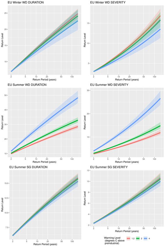
and Europe as a whole, are explored and discussed. A statistical EVA6 is then carried out to quantify
the return period of events (e.g. 1 in 10 year event) at different future global warming levels, and an
approach for using this quantification to select relevant events from the final dataset is presented.
6A glossary of acronyms is presented in Section 8
c Crown Copyright 2021, Met Office 14 of 854.1 Data sources
4.1.1 DePreSys Hindcasts
The Met Office Decadal Prediction System (DePreSys)7 has been used to produce a hindcast (ret-
rospective forecast) dataset. This is made up of global ocean-atmosphere simulations, run freely for
many ‘model’ months to produce new outcomes away from observations. Specifically, the model has
been run 40 times for each year 1959 - 2015, initialised in November. This provides 2280 model years
of plausible weather, more than 40 times the data available from the ERA5 reanalysis dataset, which
is representative of the observed historical conditions only. The DePreSys dataset has been found to
produce ‘unseen’ but plausible meteorologist conditions, more extreme than those seen in the histori-
cal record (Thompson et al., 2017). By applying the WDI and SGI to the DePreSys dataset, plausible
adverse weather events, more extreme than those observed in the historical period, could be identified,
providing additional relevant relevant for resilience testing (see Section 4.3). In addition, incorporat-
ing adverse weather events identified within these 2280 years greatly increases the size of the sample
used in the statistical EVA, reducing the uncertainty in high return period estimated (see Section 4.4).
It should be noted, however, that because the hindcasts are re-initialised each year based on observed
conditions (e.g. the observed sea surface temperature), they are not a full expression of the possible
natural variability in the ocean-atmosphere system. That is, they are not run freely for the full 57 year
period, and hence may underestimate the true climate variability.
The DePreSys data set contains mean daily 60km gridded data for the following weather variables:
1. Surface air temperature;
2. Wind ‘U’ (east-west) and ‘V’ (north-south) components at 10m above the ground, which can be
used to calculate 10m above ground wind speed8 ;
3. Mean Sea Level Pressure.
As described in Section 3, for this study, weather dependent electricity demand is calculated from
surface temperature, wind generation from 100m wind speed, and solar generation from solar radiation
and surface temperature. These energy demand and generation values are then used to calculated
the WDI and SGI, allowing for adverse weather events can be identified. Therefore, to allow for the
DePreSys dataset to be used within this study, 100m above ground wind speed and solar radiation
must be estimated coherently with the available meteorological variables. The methods developed for
this, and for calibrating the existing variables, are explained and validated in Section 4.2.
7 https://www.metoffice.gov.uk/research/approach/modelling-systems/unified-model/climate-models/depresys
(Accessed 01/06/2021)
8 http://colaweb.gmu.edu/dev/clim301/lectures/wind/wind-uv (Accessed 19/05/2021)
c Crown Copyright 2021, Met Office 15 of 854.1.2 UK Climate Projections 2018 (UKCP18)
The United Kingdom Climate Projections (UKCP18) provide the most recent assessment of how the
climate may change in the future (Lowe et al., 2018). They are based on the latest peer-reviewed
climate science, inclusive of model data from both the Met Office Hadley Centre and other international
climate-modelling centres. There are 28 global climate model (GCM) simulations providing worldwide
coverage at a 60km horizontal resolution for the historical and future periods from 1900-2100. They are
separated into two ensembles as they sample uncertainty in different ways:
1. The perturbed physics ensemble (PPE) is made up of 15 variants of the Met Office Hadley Centre
model (hereafter referred to as PPE-15). The PPE-15 is created by perturbing a set of parameters
within a single land/ocean model to sample a broad range of future outcomes in a systematic way.
2. The Coupled Model Intercomparison Project (CMIP) ensemble is made up of 13 models, produced
by 13 separate institutions, from CMIP Phase 5 (hereafter referred to as CMIP-13). Since the
models are created independently there is more scope to sample different sources of uncertainty.
The PPE-15 ensemble allows for a quantification of uncertainty owing to parameter uncertainties (how
fast ice falls in clouds, for example), while the CMIP-13 ensemble allows for a quantification of uncer-
tainties owing to structural model choices (the type of land and ocean models used, for example).
The availability of individual variables from CMIP-13 is dependent on whether the data was saved out
by the institution. Unfortunately, daily and monthly solar radiation data is not available from any of the
CMIP-13 models, wind speed is unavailable for four models and over an insufficient time period for a
fifth. Due to these data availability issues, and in order to maintain consistency across the demand, wind
and solar generation models in the uncertainty sampled, only the PPE-15 ensemble is used in this study.
Note that UKCP18 also has a suite of 12 regional climate model (RCM) simulations available at a
12km horizontal resolution; driven by 12 of the global PPE-15, which are dynamically downscaled.
These have not been used in this study: whilst these simulations do provide additional value by better
resolving physiographic features and simulating daily spatial detail of meteorological variables (Murphy,
J. M. et al., 2018), the analysis at regional level looking at long duration events does not require such
level of detail, and maintaining consistency in the resolution with other datasets of meteorological data
is of a higher priority (the DePreSys dataset and ERA5 regridded data used for bias correction in the
next section are both at a 60km resolution). Furthermore, there is a small reduction in the uncertainty
sampled in the RCM suite (12 simulations rather than 15).
4.2 Data calibration
While these data sources provide a number of advantages in their representation of additional plausible
weather years and the effect of climate change, they pose limitations in terms of climate model biases,
c Crown Copyright 2021, Met Office 16 of 85the availability of meteorological variables, and spatial and temporal resolution. As a results, the De- PreSys and UKCP18 data must undergo calibration to ensure they are fit for purpose. Throughout, the data calibration uses the ERA5 reanalysis dataset as the observed ‘truth’. The ERA5 data is on a 30km-hourly spatial-temporal resolution, and hence is regridded and temporally averaged to the same 60km-daily resolution as the DePreSys and UKCP18 datasets to allow for a direct comparison within this calibration. Bilinear interpolation9 is used to regrid the ERA5 temperature, wind speed and mean sea level pressure data, while an area-weighted method10 is used for solar radiation to ensure that the amount of radiative flux received over an area is preserved. In addition, the ERA5 100m wind speeds have been corrected using the Global Wind Atlas (as in Bloomfield et al. (2019) and descried in Dawkins and Rushby (2021)). 4.2.1 Bias correction of 10m wind speed, surface temperature and mean sea level pressure Both the DePreSys and UKCP18 datasets are derived from climate models, which are imperfect repre- sentations of the physical climate system. As such, this data is likely to contain biases when compared to observations, for example conditions may be generally too hot or too windy. DePreSys When identifying adverse weather scenarios within the DePreSys hindcasts, surface temperature will be used to calculate energy demand; 10m wind speed data will be used to estimate 100m wind speed (see Section 4.2.2), which will be used to calculate wind renewable generation; and mean sea level pressure will be used to produce fields of solar radiation that are coherent with the other DePreSys variables (see Section 4.2.3), which will subsequently be used to calculate solar renewable generation. Therefore, within the DePreSys hindcast dataset, surface temperature, 10m wind speed and mean sea level pressure must be bias corrected. Figure 3 shows the difference in the grid cell daily mean (average) and standard deviation (variabil- ity) of surface temperature, 10m wind speed and mean sea level pressure, when calculated based on the ERA5 data and the DePreSys hindcast data for all January days in the period 1979-2018. These plots show how, for example, the DePreSys data is biased to being too cold on average in some parts of Europe (particularly Norway), and not windy enough on average over much of the North Sea and Scandinavia. A variance scaling method is used to bias correct the data (see section 3.1.6 of Luo et al. 2018). This form of univariate bias correction method adjusts the mean and standard deviation of the DePreSys data 9 https://www.sciencedirect.com/topics/engineering/bilinear-interpolation (Accessed 29/04/2021) 10 https://scitools.org.uk/iris/docs/v1.10.0/userguide/interpolation_and_regridding.html$# $area-weighted-regridding (Accessed 29/04/2021) c Crown Copyright 2021, Met Office 17 of 85
Figure 3: Spatial maps of the difference between the DePreSys and ERA5 grid cell mean (a,c,e) and standard deviation (b,d,e) for surface tempera-
ture (top row), 10m wind speed (middle row) and mean sea level pressure (bottom row), for all January days in the period 1979-2018. In each case
the difference is calculated as DePreSys minus ERA5, meaning that a value above zero implies the DePreSys data is bias to being too high, and a
value below zero implies the DePreSys data is bias to being too low.

in each grid cell and meteorological variable separately, such that it is equal to the mean and standard
deviation of the equivalent grid cell and variable in the ERA5 data. The biases in the DePreSys data
vary with the time of the year, hence this bias correction is applied to each month of the year separately
(i.e. all January days in the period separately from all February days).

Figure 4 demonstrates this bias correction in each variable in January, for a single grid cell in the UK.
These plots show how the distribution of the DePreSys data (orange) is adjusted by the variance scaling
method to ensure the mean and standard deviation is consistent with the distribution of the equivalent
ERA5 data (blue). For example, in Figure 4 (a) and (b), the DePreSys data is shifted slightly to the right
to increase temperatures and wind speed, both identified as being biased too low on average compared

c Crown Copyright 2021, Met Office                                                                                                   18 of 85
Figure 4: For (a) surface temperature (b) 100m wind speed and (c) mean sea level pressure, histograms comparing the distribution of ERA5 and
DePreSys January data in a single UK grid cell, for the original (non-bias corrected) DePreSys daat (left), and for the bias corrected DePreSys data
(right).

c Crown Copyright 2021, Met Office                                                                                                      19 of 85
to ERA5 in Figure 3.

The bias correction method applied here is a univariate method, meaning that it is applied to each grid
cell and variable separately. This makes the assumption that the temporal, spatial and inter-variable
dependence in the DePreSys data is physically consistent and hence does not need to be corrected.
This assumption is thought to be reasonable because the DePreSys data is derived from a physical cli-
mate model. Multivariate bias correction methods allow for multiple variables and locations to be biased
corrected together, also allowing any biases in these dependences to be corrected. The application of
such methods to large climate and weather datasets (such as these) is known to be computationally
challenging and cause over-fitting (Cannon, 2018), and hence applying such methods was found to be
beyond the scope of this study. The final DePreSys weather data, used to identify adverse weather
scenarios, derived from the data bias corrected here are comprehensively validated in Section A.1,
showing how the temporal, spatial and inter-variable dependences in the ERA5 data are captured well
by the calibrated DePreSys data. These plots (Figures 31 - 42) show that applying a univariate bias
correction does not cause any unusual dependence structures within the resulting data.

UKCP18

For the UKCP18 data, the bias correction is achieved using a ‘built-in’ approach within the statisti-
cal EVA applied to the adverse weather scenarios (explained further in Section 4.4 and based on the
method of Brown et al. (2014)). This EVA bias correction method is applied to the duration/severity of
adverse weather events themselves rather than the underlying meteorological variable. However, since
wind generation is calculated from wind speed data using a non-linear wind power curve (Figure 1), any
biases in the wind speed data will be greatly amplified by the power curve. For this reason, the UKCP18
10m wind speed data is bias correct prior to identifying the adverse weather events. The same variance
scaling method is used to bias correct this 10m wind speed data from UKCP18, using ERA5 as the truth.

In addition, the variance scaling bias correction method assumes stationarity (i.e. that the variable
being corrected is not systematically changing over time). This assumption is seen to be acceptable for
UKCP18 wind speed data, which does not show a clear change in the future in the UKCP18 projections
(Lowe et al., 2018), but would not be acceptable for UKCP18 surface temperature, which has been
shown to increase in the future (Lowe et al., 2018; Murphy, J. M. et al., 2018). This therefore neces-
sitates the bias correction of UKCP18 surface temperature using an alternative approach which allows
for non-stationarity (changes over time) to be retained, such as the EVA approach described above and
in Section 4.4.

Applying the variance scaling bias correction to UKCP18 10m wind speed data achieves equivalent
consistencies with the mean and standard deviation of ERA5 as shown for DePreSys in Figure 4. This

c Crown Copyright 2021, Met Office                                                             20 of 85
Figure 5: Spatial maps of the mean 10m wind speed in each 60 km grid cell, calculated for (a) ERA5, (b) bias corrected DePreSys and (c) bias
corrected UKCP18, over the full period of each dataset.

is evidenced in the similarity between the ERA5 and UKCP18 mean 10m wind speed across Europe in
Figure 5 (a) and (c), also consistent with the DePreSys 10m wind speed mean shown in Figure 5 (b).

4.2.2    Representing 100m wind speed

Wind generation calculations require turbine height wind speeds, generally around 100m above ground.
The wind speed data available in DePreSys and UKCP18 is 10m above the ground, so a method must
be developed to scale this wind speed data to the 100m above ground height. Existing methods such
as the log law11 and power law12 can be used to scale wind speed from one height to another, however
these make assumptions about the surface roughness or wind shear exponent. In addition, discussions
with experts within the Met Office highlighted how these laws may not hold as well for low wind speeds,
which are particularly important when investigating wind droughts in this study.

An alternative approach, commonly used to correct and adjust wind data (e.g. Dunstan et al. 2016), is
to employ a data science modelling technique to represent the relationship between the two wind speed
heights (here 10m and 100m) within a dataset that contains both levels (e.g. ERA5), and then use this
relationship to scale the data within another dataset that just contains one level (here DePreSys and
UKCP18). In this case, a data science method known as Generalised Additive Modelling (GAM)13 is
used. This type of model aims to represent a response/target variable (here 100m wind speed) using a
combination of smooth functions of other variables (e.g. 10m wind speed).

Figure 6 shows the relationship between daily mean 10m and 100m above ground wind speed, taken
from the ERA5 dataset, for a single 60 × 60 km grid cell. This figure shows how there is a strong linear
relationship between 10m and 100m wind speed, that varies slightly by season. To capture these ob-
served relationships, the GAM is structured such that the response/target variable (100m wind speed)
is estimated based on 10m wind speed and ‘day of the year’. Additional explanatory variable are also
included to help improve the predictability of the model (i.e. how well 100m wind speed is estimated
from other variables). Since the aim it to apply the GAM to the DePreSys data to allow for 100m wind
  11 http://www.met.reading.ac.uk/
                                  ~marc/it/wind/interp/log_prof/ (Accessed 02/06/2021)
  12 https://websites.pmc.ucsc.edu/
                                   ~jnoble/wind/extrap/ (Accessed 02/06/2021)
  13 https://datascienceplus.com/generalized-additive-models/ (Accessed 24/05/2021)

c Crown Copyright 2021, Met Office                                                                                              21 of 85
Figure 6: The relationship between daily average 10m and 100m (above ground) wind speed, taken from ERA5 (bias corrected and re-gridded as explained at the beginning of Section 4.2 and Section 4.2.1), for the period 01/01/1979 - 31/12/2018 in a single 60 × 60 km grid cell. Each data point is a day within the record, and each is coloured according to the season that day falls in: Autumn (Sept-Nov), Winter (Dec-Feb), Spring (Mar-May) and Summer (Jun-Aug). speed to be estimated for this dataset, these additional variables must be available within the DePreSys hindcasts (see Section 4.1.1). Hence, the grid cell surface temperature and the year are included as additional explanatory variables. In addition, the relationship between 10m and 100m wind speed is found to vary with location (due to differences in surface orography). For this reason, a separate GAM model is trained for each grid cell in the European domain. Figure 7 presents an example of the GAM, trained on the ERA5 data in a single grid cell. The four plots shows the smooth function fitted to each of the explanatory variables (10m wind speed, tempera- ture, day of the year and year). These show how, as well as the strong relationship between 10m and 100m wind speed seen in Figure 6, there is a linear relationship between temperature and 100m wind speed (as temperature increases so does 100m wind speed), and a non-linear relationship with the day of the year (100m wind speed is generally lower in summer/autumn). Similar relationships are found in other grid cells. These four smooth functions can be used to predict 100m wind speed based on these four variables, by summing f(variable), where the value of the variable is representative of that given day (i.e. the 10m wind speed, temperature, day of year and year). A cross-validation method is used to validate this model. The GAM is trained on a subset of the ERA5 data (80%), and then used to estimate 100m wind speed for the remaining 20% of the (un-modelled) test data. An example of the relationship between the predicted and true 100m wind speed in one grid cell is presented in Figure 8 (a). This shows how the model is able to very accurately estimate 100m wind speed from the four explanatory variables. Specifically, in this grid cell 98.8% of the variance in the 100m wind speed data is explained by the GAM model, with 100% equating to perfect predictability. A similarly high proportion of the variance is explained (high predictability is achieved) in GAMs trained c Crown Copyright 2021, Met Office 22 of 85
Figure 7: A graphical representation of the the Generalised Additive Model trained on ERA5 data in a single grid cell. Each of the four plots
shows the smooth function fitted to each of the explanatory variables (10m wind speed, temperature, day of the year and year), which are used in
combination (summed together) to estimate the response/target variable (100m wind speed). In each plot the ticks along the x axis show where the
data lies along this dimension.

Figure 8: (a) Scatter plot of ‘true’ daily average 100m wind speed from ERA5, and the associated predicted daily average 100m wind speed from
the GAM based on 10m wind speed, surface temperature, day of the year and the year, for the cross validation test data in grid cell: longitude 2.5
and latitude 51.7. (b) A map of the proportion of variance in 100m wind speed explained the GAM fitted to each variable in the UK region, where a
value of 0.996 represents 99.6% of the variance being explained. This value is also know as the coefficient of determination or R-squared.

on each grid cell of the European region, a subset of which are shown in Figure 8 (b).

c Crown Copyright 2021, Met Office                                                                                                    23 of 85
Figure 9: Spatial maps of the mean 100m wind speed in each 60 km grid cell, calculated for (a) ERA5, (b) predicted from GAM for DePreSys and
(c) predicted from GAM for UKCP18, over the full period of each dataset.

These grid cell GAMs are subsequently applied to the 2280 model years of DePreSys historical hind-
cast data. The bias corrected daily mean surface temperature and 10m wind speed (see Section 4.2.1)
are used with the temporal variables ‘day of the year’ and ‘year’, within the GAM smooth functions, to
predict the associated daily mean 100m wind speed value. As shown in Figure 9 (a) and (b), this pro-
vides DePreSys 100m wind speed values that are consistent on average with ERA5 data, and hence
can be used to estimate wind generation within this study. This estimated 100m wind speed data is
further validated in Section A.1. Figures 31 - 42 show how the inter-variable, spatial and temporal vari-
ability of this estimated DePreSys 100m wind speed data is very similar to that seen in the ERA5 record.

Figure 10: Scatter plot of ‘true’ daily average 100m wind speed from ERA5, and the associated predicted daily average 100m wind speed from the
GAM based on 10m wind speed and moth of the year, for the cross validation test data in grid cell: longitude 2.5 and latitude 51.7.

In a similar way, the UKCP18 daily average 10m wind speed data is scaled to the 100m level. In this
case, a slightly different GAM is trained on the ERA5 data. This must be done because the UKCP18 sur-
face temperature data has not yet been bias corrected (as explained in Section 4.2.1), hence it cannot
be used as an input in the GAM. In addition, the UKCP18 data is produced on a 360-day calendar, to the
year 2098, meaning that the ‘day of the year’ is not consistent with ERA5, and the ERA5 ‘year’ variable
doesn’t capture all of the UKCP18 years. Instead, the GAM is structured such that the response/target

c Crown Copyright 2021, Met Office                                                                                                24 of 85
You can also read