The northern European shelf as an increasing net sink for CO2 - Biogeosciences
←
→
Page content transcription
If your browser does not render page correctly, please read the page content below

Biogeosciences, 18, 1127–1147, 2021
https://doi.org/10.5194/bg-18-1127-2021
© Author(s) 2021. This work is distributed under
the Creative Commons Attribution 4.0 License.

The northern European shelf as an increasing net sink for CO2
Meike Becker1,2 , Are Olsen1,2 , Peter Landschützer3 , Abdirhaman Omar4,2 , Gregor Rehder5 , Christian Rödenbeck6 ,
and Ingunn Skjelvan4,2
1 Geophysical   Institute, University of Bergen, Bergen, Norway
2 Bjerknes Center for Climate Research, Bergen, Norway
3 Max Planck Institute for Meteorology, Hamburg, Germany
4 NORCE Norwegian Research Centre AS, Bergen, Norway
5 Leibniz Institute for Baltic Sea Research, Warnemünde, Germany
6 Max Planck Institute for Biogeochemistry, Jena, Germany

Correspondence: Meike Becker (meike.becker@uib.no)

Received: 4 December 2019 – Discussion started: 14 January 2020
Revised: 30 October 2020 – Accepted: 5 November 2020 – Published: 15 February 2021

Abstract. We developed a simple method to refine exist-          1   Introduction
ing open-ocean maps and extend them towards different
coastal seas. Using a multi-linear regression we produced
monthly maps of surface ocean f CO2 in the northern Euro-        For facing global challenges, such as predicting and tracking
pean coastal seas (the North Sea, the Baltic Sea, the Norwe-     climate change, it is important to improve our understand-
gian Coast and the Barents Sea) covering a time period from      ing of the ocean carbon sink and its variability. Open oceans,
1998 to 2016. A comparison with gridded Surface Ocean            especially those of the Northern Hemisphere, are relatively
CO2 Atlas (SOCAT) v5 data revealed mean biases and stan-         well understood and described in their large-scale variability
dard deviations of 0 ± 26 µatm in the North Sea, 0 ± 16 µatm     (Gruber et al., 2019; Landschützer et al., 2018, 2019; Fay and
along the Norwegian Coast, 0 ± 19 µatm in the Barents Sea        McKinley, 2017). Reliable autonomous systems for measur-
and 2 ± 42 µatm in the Baltic Sea. We used these maps to         ing carbon dioxide partial pressure from commercial vessels
investigate trends in f CO2 , pH and air–sea CO2 flux. The       were developed in the early 2000s (Pierrot et al., 2009) and
surface ocean f CO2 trends are smaller than the atmospheric      have since been deployed on a large number of vessels (e.g.,
trend in most of the studied regions. The only exception to      Bakker et al., 2016). This has resulted in sufficient data to de-
this is the western part of the North Sea, where sea surface     velop methods to interpolate the data and to describe large-
f CO2 increases by 2 µatm yr−1 , which is similar to the at-     scale air–sea CO2 exchange and its variability (Landschützer
mospheric trend. The Baltic Sea does not show a signifi-         et al., 2014, 2013; Rödenbeck et al., 2013; Jones et al., 2015).
cant trend. Here, the variability was much larger than the ex-   These methods apply a wide variety of approaches, such as
pected trends. Consistently, the pH trends were smaller than     linear interpolation, machine learning and model-based es-
expected for an increase in f CO2 in pace with the rise of       timates. By comparing the different results, it is possible to
atmospheric CO2 levels. The calculated air–sea CO2 fluxes        achieve a good estimate of the uncertainty associated with
revealed that most regions were net sinks for CO2 . Only         the respective methods (Rödenbeck et al., 2015).
the southern North Sea and the Baltic Sea emitted CO2 to            Despite coastal seas covering 7 %–10 % of the world’s
the atmosphere. Especially in the northern regions the sink      oceans (Bourgeois et al., 2016), their contribution to the
strength increased during the studied period.                    oceanic carbon sink is not yet fully constrained. Whether
                                                                 coastal seas are a net sink or source for atmospheric CO2
                                                                 and how their role will change in a changing climate is still
                                                                 under debate (Bauer et al., 2013; Laruelle et al., 2010). Com-
                                                                 pared to the open ocean, longer time series and higher spatial
                                                                 and temporal resolution of the observations are needed in or-

Published by Copernicus Publications on behalf of the European Geosciences Union.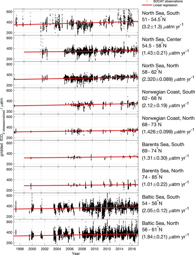
1128                                                                                               M. Becker et al.: Coastal f CO2 maps

Table 1. Overview of trends in surface ocean CO2 reported in the literature.

                     Reference                        Time range                            dpCO2 /dt (µatm yr−1 )
 North Sea           Thomas et al. (2007)             2001–2005, summer data,               7.9
                                                      normalized to 16◦
 North Sea           Salt et al. (2013)               2001–2005, summer data,               6.5
                                                      normalized to 16◦
 North Sea           Salt et al. (2013)               2005–2008, summer data,               1.33
                                                      normalized to 16◦
 Faroe Banks         Fröb et al. (2019)               2004–2017, winter data (DJFM)         2.25 ± 0.20
 North Sea, west     Omar et al. (2019)               2004–2017, winter data (DJ)           2.19 ± 0.55
 North Sea, east     Omar et al. (2019)               2004–2017, winter data (DJF)          not significant
 North Sea           Laruelle et al. (2018)           1988–2015                             almost no trend
 English Channel     Laruelle et al. (2018)           1988–2015                             slightly smaller than atmosphere
 Baltic Sea          Wesslander et al. (2010)         1994–2008                             larger than atmosphere
 Baltic Sea          Schneider and Müller (2018)      2008–2015                             4.6–6.1
 Baltic Sea, west    Laruelle et al. (2018)           1988–2015                             much smaller than atmosphere, slightly negative
 Barents Sea         Yasunaka et al. (2018)           1997–2013                             not significant
 Barents Sea         Laruelle et al. (2018)           1988–2015                             about the same as atmosphere
 Atmosphere          global average                   1997–2016                             2.02 ppm yr−1

Table 2. Overview of air–sea CO2 fluxes reported in the literature. Negative sign denotes flux from atmosphere to ocean.

                                                  Reference                    Time range    F (mmol m−2 d−1 )
                             North Sea            Meyer et al. (2018)          2001/02                    −3.8
                             North Sea            Kitidis et al. (2019)        2015                     0– −15
                             Baltic Sea           Parard et al. (2017)         1998–2011                    1.2
                             Norwegian Coast      Yasunaka et al. (2018)       1997–2013                −4– −8
                             Barents Sea          Yasunaka et al. (2018)       1997–2013               −8– −12

der to capture all relevant coastal processes. Small-scale cir-               The different maps developed for describing the open-
culation patterns governed by topographic features; thermal                ocean surface pCO2 (CO2 partial pressure) dynamics and
and haline stratification; or mixing through tidal cycles, up-             air–sea CO2 fluxes are not directly applicable in coastal re-
welling or internal waves result in a need for more complex                gions. Many exclude data from continental shelves com-
maps with a higher resolution (Bricheno et al., 2014; Lima                 pletely while all of them have too coarse a spatial resolu-
and Wethey, 2012; Blanton, 1991). These physical drivers                   tion (typically between 1 and 5◦ ) to properly resolve coastal
are not the only reasons for coastal seas being more compli-               seas with their small-scale variability. A few studies have
cated to understand. Generally, coastal regions are more pro-              described coastal carbon dynamics, but most of them have
ductive than open-ocean regions due to better availability of              strong regional or temporal limitations. Table 1 shows an
nutrients (e.g., mixing at continental margins, river runoff).             overview of studies with estimated pCO2 trends over the
While deeper coastal regions are seasonally stratified, shal-              northern European shelf, while Table 2 presents available
low regions are vertically mixed, allowing for exchange be-                flux estimates. Laruelle et al. (2017) used a neural net-
tween the benthic and pelagic parts of the ecosystem (Grif-                work approach to produce a global pCO2 climatology for
fiths et al., 2017; Wollast, 1998). Together with strong gradi-            coastal seas, describing more distinct seasonal variability in
ents of productivity this leads to spatial and temporal hetero-            the Northern Hemisphere than in the southern Pacific and At-
geneity in surface CO2 content.                                            lantic. A global climatology covering both open-ocean and
                                                                           coastal regions was recently constructed by combining this

Biogeosciences, 18, 1127–1147, 2021                                                            https://doi.org/10.5194/bg-18-1127-2021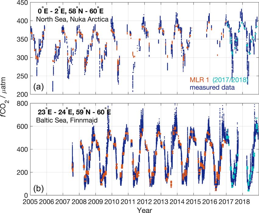
M. Becker et al.: Coastal f CO2 maps                                                                                       1129

product with the open-ocean product of Landschützer et al.
(2016, 2020). Laruelle et al. (2018) published trend estimates
in regions with high data coverage based on winter data span-
ning up to 35 years. Their findings is that the pCO2 rise
in coastal regions tends to lag the atmospheric rise in CO2 .
However, few studies attempted to constrain coastal air–sea
fluxes before. Kitidis et al. (2019) estimated fluxes between 0
and −15 mmol m−2 d−1 in the North Sea, depending on the
season (more negative during summer than during winter)
and the region (more negative fluxes in the northern North
Sea compared to the south). For the Baltic Sea, Parard et al.
(2016, 2017) used a neural network approach to produce sur-
face ocean pCO2 maps from 1998 to 2011 and estimated
an air–sea flux of 1.2 mmol m−2 d−1 . Yasunaka et al. (2018)
estimated a flux of 8–12 mmol m−2 d−1 in the Barents Sea
and along the Norwegian Coast using a self-organizing map
technique. Most of the other available studies on the trends
in coastal pCO2 are based on data from either summer or
winter. Estimates based on summer-only data typically show
large interannual variations (Thomas et al., 2007; Salt et al.,
2013), which led to the conclusion that here the interannual      Figure 1. The study area and the location of the four different
variability masks the actual long-term trend. The approach        regions: North Sea (purple), Norwegian Coast (red), Barents Sea
to use winter-only data (Fröb et al., 2019; Omar et al., 2019),   (green) and Baltic Sea (blue).
however, is based on the assumption that during this season
the influence of biological processes is negligible and there-
fore winter data can be used to establish a baseline trend.       coverage in these regions is fairly high and (2) the authors
However, also using winter-only data has its drawbacks. In        have strong knowledge of the specific regions. This is im-
particular the choice of which months to include can cause        portant in order to properly evaluate the maps and to as-
biases, and the optimal selection can differ from region to       sess whether or not the output is realistic. The four regions
region.                                                           were defined based on the COastal Segmentation and re-
   In this study we present a new approach to develop             lated CATchments (COSCAT) segmentation scheme (Laru-
monthly f CO2 (CO2 fugacity) maps based on already ex-            elle et al., 2013). The threshold for defining a region as
isting open-ocean pCO2 maps in four example regions: the          coastal sea was set to a depth limit of 500 m. By using this
North Sea, the Baltic Sea, the Norwegian Coast and the Bar-       definition, we produce an overlap to the open-ocean maps,
ents Sea. A multi-linear regression (MLR) was used to fit         allowing our maps to be merged with the open-ocean maps.
driver data against f CO2 observations. Based on the result-      Please note that this study concentrates on the continental
ing f CO2 maps and a salinity–alkalinity correlation we also      shelf area. The near-coastal zones (e.g., intertidal zones) are
produced monthly maps of coastal pH. The performance of           not included due to the limited availability of driver data in
the produced maps was evaluated, and the maps were then           these regions.
used to investigate trends in coastal f CO2 and pH in the en-
tire region from 1998 to 2016. Finally, we used the f CO2         2.2   Data handling
maps to determine the air–sea CO2 exchange and its tempo-
ral and spatial patterns.                                         The CO2 data used in this study were extracted from Sur-
                                                                  face Ocean CO2 Atlas (SOCAT) version 5 (Bakker et al.,
                                                                  2016). Their coverage is shown in Fig. 2. A newer version
2     Method                                                      of the SOCAT database (SOCATv2019) was used for vali-
                                                                  dating the maps against independent data. An overview over
2.1    Study area                                                 the reanalysis products used as driver data is given in Ta-
                                                                  ble 3. We use as basic driver data sea surface temperature
This work focuses on the northern European continental shelf      (SST), sea surface salinity (SSS), chlorophyll a concentra-
and marginal seas. As we want to show the performance of          tion (Chl a), mixed layer depth (MLD), bathymetry (BAT),
the MLR method we picked a number of regions with very            distance from shore (DIST), ice concentration (ICE) and the
different characteristics: the North Sea, the Baltic Sea, the     change in ice concentration from the month to month (prior
Norwegian Coast and the western Barents Sea (Fig. 1). We          to current). Chl a values during the dark winter season were
decided to concentrate on these regions because (1) the data      set to 0. In addition to the reanalysis data, pCO2 values from

https://doi.org/10.5194/bg-18-1127-2021                                                  Biogeosciences, 18, 1127–1147, 2021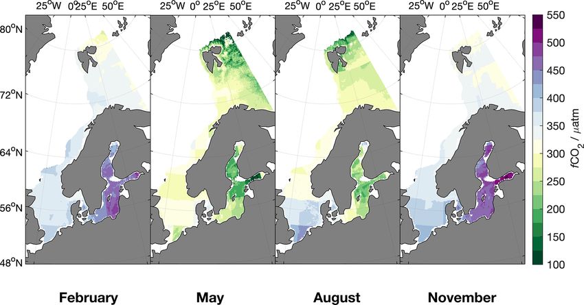
1130                                                                                           M. Becker et al.: Coastal f CO2 maps

Table 3. Products used as driver data in the MLR and the maps.

               Product used           Resolution                     Reference
               Chl a for MLR          4 km × 4 km, 8 d               Global Ocean Chlorophyll (Copernicus-GlobColour)
                                                                     from Satellite Observations – Reprocessed
               Chl a for maps         4 km × 4 km, monthly           Global Ocean Chlorophyll (Copernicus-GlobColour)
                                                                     from Satellite Observations – Reprocessed
               MLD                    12.5 km × 12.5 km, monthly     Arctic Ocean Physics Reanalysis
               ICE                    0.25◦ × 0.25◦ , monthly        Cavalieri et al. (1996)
               SST/SSS                0.25◦ × 0.25◦ , weekly         Global Ocean Observation-based Products
                                                                     Global_Rep_Phy_001_021
               BAT                    2 min × 2 min                  ETOPO2v2 Center (2006)
               Rödenbeck pCO2         5◦ × 4◦ , monthly              Rödenbeck et al. (2014)
               Landschützer pCO2      1◦ × 1◦ , monthly              Landschützer et al. (2017)

                                                                      istry fitted against surface pCO2 observations, while Land-
                                                                      schützer et al. (2016) uses a two-step neural network (a feed-
                                                                      forward network coupled with self-organizing maps, FFN-
                                                                      SOM) trained with the pCO2 observations. Please note that
                                                                      the Rödenbeck open-ocean map contains data in coastal grid
                                                                      boxes, while the Landschützer open-ocean map is restricted
                                                                      to the open-ocean regions. The MLR models based on these
                                                                      two are called MLR 1 (based on the coastal pCO2 values
                                                                      from the Rödenbeck map) and MLR 2 (based on the near-
                                                                      est open-ocean pCO2 values of the Landschützer map), re-
                                                                      spectively. To determine the extent to which the regressions
                                                                      benefit from the information in the open-ocean maps, a third
                                                                      MLR, MLR 3, was determined. Here, we do not use any of
                                                                      the open-ocean maps as a driver, but to account for the annual
                                                                      rise in CO2 , year is included in the set of driver data.
                                                                         For preparing the input data for the MLR, observations
                                                                      closest to each SOCAT f CO2 data point in time and space
                                                                      were extracted from the 3-D fields with the driver data. This
                                                                      produces, for each of the driver data, a vector as long as the
                                                                      SOCAT f CO2 observations. After this, the f CO2 data as
Figure 2. The number of months with f CO2 data from SOCAT v5          well as all extracted driver data were binned on a monthly
in each grid box. The data cover a range of 20 years (240 months).    0.125◦ × 0.125◦ grid covering 1997 to 2016. These proce-
                                                                      dures ensure that the driver data have the same bias in space
                                                                      and time within each grid box as the f CO2 data. If a grid
                                                                      box for example only contains f CO2 observations from the
the closest coastal grid cell of the open-ocean map were used         first week of the month and the northwestern corner, we make
as a driver in our MLR. We neglect the approximately 1 µatm           sure that also the gridded driver data only contain values from
difference between partial pressure (reported in the mapped           the first week and the northwestern corner of the grid box,
products) and fugacity of CO2 (reported in SOCAT) as it is            and not an average over the entire month and grid box. This
much smaller than the accuracy of the data extracted from             is mostly important for the chlorophyll driver data, which are
SOCAT v5 (2 to 10 µatm) and the uncertainty associated                available at a very high resolution compared to the f CO2
with the open-ocean maps. The open-ocean pCO2 values                  maps produced in this work. These driver data were used for
were extracted from two different products (Rödenbeck et al.,         determining the MLRs.
2014, version oc_v1.5; and Landschützer et al., 2017, 2016,              For producing the final maps, a second set of the driver
version 2016). Rödenbeck et al. (2014) is based on a data-            data was prepared, which is called field data in the fol-
driven diagnostic model of mixed layer ocean biogeochem-

Biogeosciences, 18, 1127–1147, 2021                                                        https://doi.org/10.5194/bg-18-1127-2021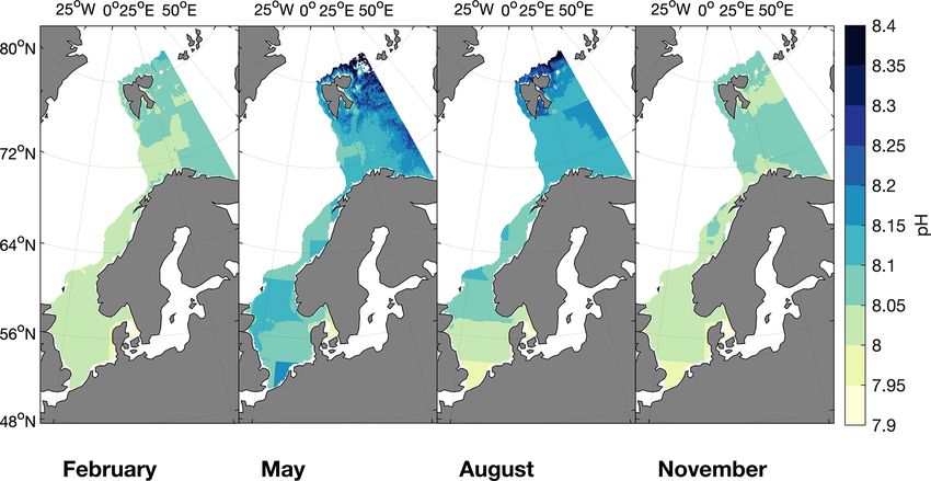
M. Becker et al.: Coastal f CO2 maps                                                                                          1131

lowing. Here the driver data were directly regridded to a           data that were not used to produce the maps, we predicted
monthly 0.125◦ × 0.125◦ grid, providing full spatial and tem-       the f CO2 for the years 2017 and 2018 (i.e., we applied
poral coverage and a homogeneous average in each grid box.          the trained multi-linear model to driver data from 2017 and
The field data were used to produce the f CO2 maps based            2018) and compared these maps to f CO2 observations in
on the MLR equations.                                               SOCAT v2019, gridded on a monthly 0.125◦ × 0.125◦ grid.
                                                                    We also compare the maps directly with observations from
2.3    Multi-linear regression                                      repeated sampling locations in the North Sea and the Baltic
                                                                    Sea.
The multi-linear regression models were constructed by for-
ward and backward stepwise regression using the driver data         2.5   Ocean acidification
as predictor variables to model the f CO2 observations. In
each step of this regression procedure, the model’s tolerance       For calculating the pH, alkalinity (AT) was estimated in the
to addition or exclusion of a variable is tested. This decision     North Sea, along the Norwegian Coast, and in the Barents
on whether to add or remove a term is based on the p value of       Sea via a salinity–alkalinity correlation following Nondal
the F statistic with or without the term in question. The en-       et al. (2009). Alkalinity describes the capacity of the sea wa-
trance tolerance was set to 0.05 and the exit tolerance to 0.1.     ter to buffer changes in pH. As the concentration of most of
The model includes constant, linear, and quadratic terms as         the weak bases in seawater is strongly dependent on the salin-
well as products of linear terms. Equation (1) gives the basic      ity, alkalinity can in many regions be estimated from salinity.
equation, with X1 . . . Xn being the driver data and a1 . . . ann   However, in regions with a high amount of organic bases in
the regression coefficients.                                        seawater, for example in strong blooms or at river mouths,
                                                                    deviations from the alkalinity–salinity relationship can oc-
y = a0 + a1 · X1 + . . . + an · Xn + a12 · X1 X2                    cur. The carbonate system was calculated using the CO2SYS
      + . . . + amn · Xm Xn + a11 · X12 + . . . + ann · Xn2   (1)   program (van Heuven et al., 2009) with carbonic acid dis-
                                                                    sociation constants of Mehrbach et al. (1973) as refitted by
The pCO2 value of the respective open-ocean maps was                Dickson and Millero (1987), KSO−      4 dissociation constants
used for MLR 1 and MLR 2, while year was always used                following Dickson (1990) and the boron–salinity relation fol-
as a driver variable in MLR 3. Inclusion of stationary drivers      lowing Uppström (1974). For the Baltic Sea, we did not cal-
(such as month, latitude and longitude) in the MLR increased        culate pH as the alkalinity–salinity relationship in this region
the performance of MLR 2 and MLR 3. However, these were             is complex due to different AT–S relations in different sub-
still not better than MLR 1, and we therefore decided to limit      regions of the Baltic Sea and a non-negligible increase in AT
this analysis to dynamic parameters. Using dynamic drivers          over the last 25 years (Müller et al., 2016).
only assures a dynamic description of the conditions in the
field and gives us the possibility to reproduce changes caused      2.6   Calculation of trends
by a regime shifts, for example the ongoing Atlantification of
the Barents Sea (Oziel et al., 2017; Lind et al., 2018).            For calculating trends of f CO2 and ocean acidification, the
                                                                    data in every grid box were deseasonalized by subtracting the
2.4    Validation                                                   long-term averages of the respective months. Then a linear
                                                                    fit was applied to the deseasonalized time series. For illus-
The three linear fits were compared to each other in each re-       trating the influence of interannual variability we calculated
gion by taking into account the R 2 and the root mean square        the trend for different time ranges. As a time range less than
error (RMSE) of the fit, as well as the Nash–Sutcliffe method       10 years barely resulted in significant trends, we decided to
efficiency (ME) (Nondal et al., 2009). The method efficiency        limit the trend analysis to starting years 1998 through 2006
compares how well the model output (En ) fits the observa-          and ending years 2008 through 2016.
tions (In ) for every data point n to how well a simple monthly
average (I ) would fit the observations:                            2.7   Flux calculation

             (In − En )2
        P
                                                                    The air–sea disequilibrium was calculated as the difference
ME = Pn                   .                                 (2)     between our mapped f CO2 values and atmospheric f CO2
                        2
             n (In − I )
                                                                    in each grid cell and time step. The atmospheric f CO2 was
   A method efficiency > 1 means that using just monthly            determined by converting the xCO2 from the NOAA marine
averages of all data in the region would fit better to mea-         boundary layer reference product from the NOAA GMD Car-
sured data than the respective model. Generally, a method           bon Cycle Group into f CO2 by using monthly SST and SSS
efficiency > 0.8 is considered bad. Besides the statistics of       data (Table 3) and monthly air pressure data from the NCEP-
the fit itself, the final maps were also compared to the grid-      DOE Reanalysis 2 (Kanamitsu et al., 2002). We calculated
ded SOCAT v5 data, resulting in an average offset and stan-         the air–sea CO2 flux (F ) according to Eq. (3), such that neg-
dard deviation (SD). In order to compare the maps against           ative fluxes are into the ocean. The gas transfer coefficient k

https://doi.org/10.5194/bg-18-1127-2021                                                    Biogeosciences, 18, 1127–1147, 2021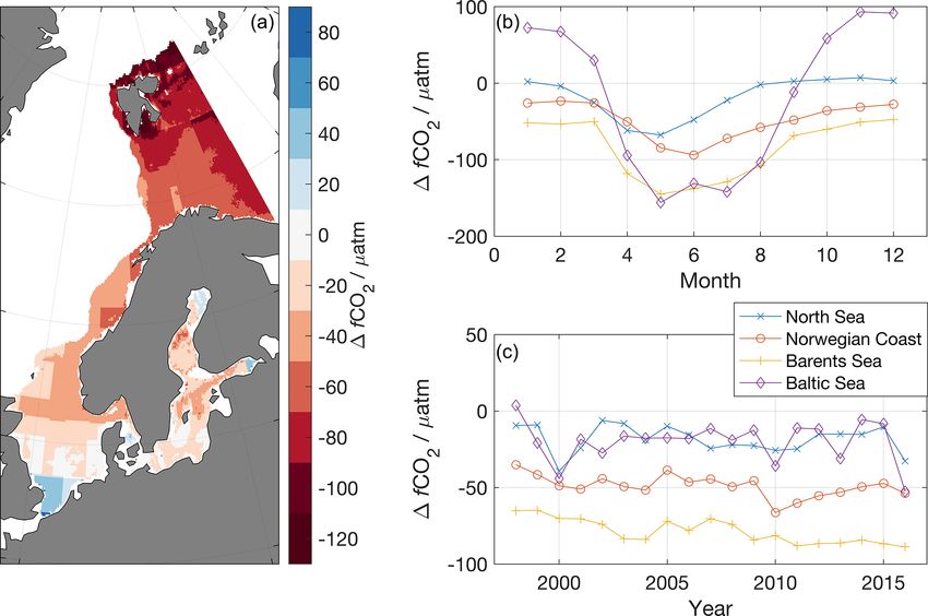
1132                                                                                       M. Becker et al.: Coastal f CO2 maps

Table 4. Driver used in the different regressions.

                                 log (MLD)     SST   SSS   CHL    ICE      ICE change   log (BAT)    DIST    pCO2    year
           North Sea
           MLR 1                      x          x    x     x      x                        x                  x
           MLR 2                      x          x    x     x      x           x            x         x        x
           MLR 3                      x          x    x     x      x           x            x         x                x
           Norwegian Coast
           MLR 1                      x          x    x     x      x                        x                  x
           MLR 2                      x          x    x     x      x           x                               x
           MLR 3                      x          x    x     x      x           x            x                          x
           Barents Sea
           MLR 1                      x          x    x     x                  x            x                  x
           MLR 2                      x          x    x     x      x           x                               x
           MLR 3                      x          x    x     x      x           x                                       x
           Baltic Sea
           MLR 1                      x          x    x     x      x           x            x                  x
           MLR 2                      x          x    x     x      x           x                               x
           MLR 3                      x          x    x     x      x                        x                          x

was determined using the quadratic wind speed (u) depen-               are provided in the Supplement. The MLRs substantially im-
dency of Wanninkhof (2014) (Eq. 4). The Schmidt number,                prove the predictions of the open-ocean maps in all studied
Sc, was calculated according to Wanninkhof (2014) and the              regions, showing a better average offset and SD to SOCAT v5
solubility coefficient for CO2 , K0 , following Weiss (1974).          and ME than the coarser-resolution open-ocean maps (for ex-
                                                                       ample the Rödenbeck map: North Sea, 0 ± 95 µatm; Norwe-
F = k · K0 · (f CO2,sw − f CO2,atm )                        (3)        gian Coast, 2 ± 17 µatm; Barents Sea, 22 ± 40 µatm; Baltic
                                                                       Sea, 4 ± 48 µatm; MLR1: North Sea, 0 ± 26 µatm; Norwe-
                    Sc −0.5

k = aq · hu2 i ·                                            (4)        gian Coast, 0 ± 16 µatm; Barents Sea, 0 ± 19 µatm; Baltic
                   660                                                 Sea, 2 ± 42 µatm). In all regions MLR 1 has the best model
   In our calculations, we used 6-hourly winds of the NCEP-            efficiency, the highest R 2 and the smallest RMSE of the fit,
DOE Reanalysis 2 product. The coefficient aq in Eq. (4) is             while these statistics are worse for MLR 2 and MLR 3. This
strongly dependent on the wind product used (Roobaert et al.,          can be explained by the fact that the Rödenbeck map contains
2018). We determined it to be aq = 0.16 cm h−1 for the 6-              information about the continental shelf and the Barents Sea,
hourly NCEP 2 product following the recommendations of                 while for MLR 2 the closest open-ocean grid cell of Land-
Naegler (2009) and by using the World Ocean Atlas sea sur-             schützer et al. (2017) was used. The fact that MLR 3 showed
face temperatures (Locarnini et al., 2018). The barrier effect         the weakest performance shows the value of using informa-
of sea ice on the flux was taken into account by relating the          tion from the open-ocean maps in the regression.
flux to the ice cover extent following Loose et al. (2009).               Figure 3 shows, from left to right, the spatial distribu-
As the gas exchange in areas that are considered 100 % ice             tion of the average difference between the predicted f CO2
covered from satellite images should not be completely ne-             by MLR 1 and the gridded SOCAT v5 data, the Rödenbeck
glected, we use a sea ice barrier effect for a 99 % sea ice            map and the gridded SOCAT v5 data, the difference between
cover in all grid cells where the sea ice coverage exceeded            MLR 1 and the Rödenbeck map, and, for comparison, the
99 %.                                                                  difference between MLR 3 and the SOCAT v5 data. In the
                                                                       North Sea, MLR 1 seems to slightly overestimate the f CO2
                                                                       in the constantly mixed region at the entrance of the English
3     Results                                                          Channel and the area off the Danish North Sea coast. In the
                                                                       Baltic, MLR 1 generally describes the spatial variability in
3.1    Maps of f CO2                                                   f CO2 well. However, in the Gulf of Finland it usually pre-
                                                                       dicts f CO2 values that are too low during May/June while it
The skill assessment metrics for MLR 1, MLR 2 and MLR 3                slightly underestimates events of very high f CO2 in Decem-
are presented in Table 5. It shows the R 2 and RMSE of the             ber/January. Regardless, the spatial biases vs. SOCAT are
fit, the ME, and the average offset and SD to the gridded SO-          clearly smaller for MLR 1 than for the original Rödenbeck
CAT data. The coefficients for MLR 1, MLR 2 and MLR 3                  map. Further, as the predictions of MLR 2 and 3 are clearly

Biogeosciences, 18, 1127–1147, 2021                                                      https://doi.org/10.5194/bg-18-1127-2021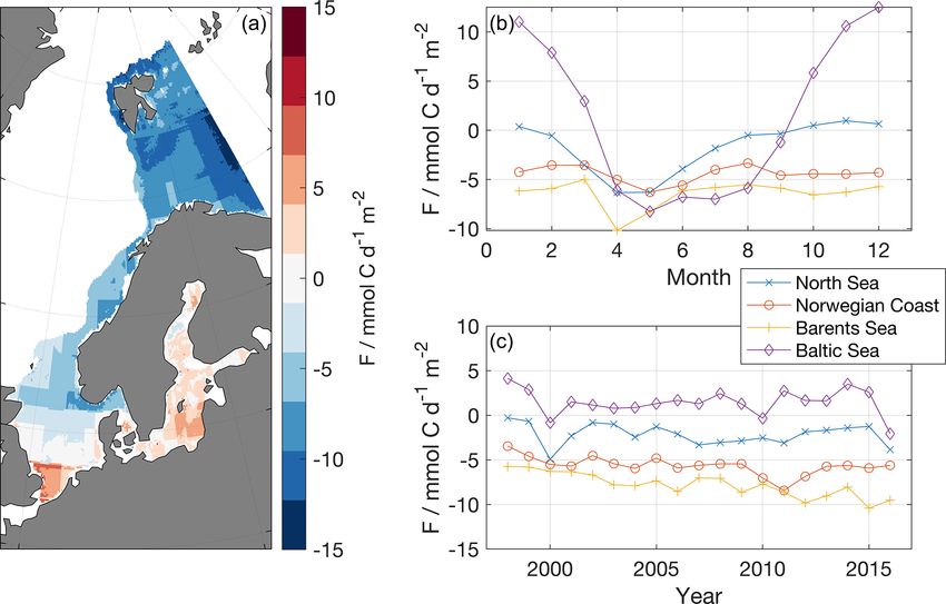
M. Becker et al.: Coastal f CO2 maps                                                                                                   1133

Table 5. Statistical evaluation of the MLR 1, MLR 2 and MLR 3 in comparison to the open-ocean maps of Rödenbeck et al. (2015) and
Landschützer et al. (2017) for each region. The data for the open-ocean map of Landschützer et al. (2017) are in parentheses since this is
based on an extrapolation of the nearest open-ocean grid cell towards the coast. The number of grid cells containing data is given behind the
region abbreviations.

                                                 R 2 adj   RMSE       ME       difference to gridded SOCAT v5
                                                                    median      mean                       SD
                                                           (µatm)              (µatm)                   (µatm)
                             North Sea (36170)
                             MLR 1             0.7271         25    0.3145     −0.15                         26
                             MLR 2             0.5130         33    0.5789     −0.52                         36
                             MLR 3             0.5331         33    0.4895      −2.4                         32
                             Rödenbeck                              0.3522     −0.28                         95
                             (Landschützer)                         0.5714      −4.7                        103
                             Norwegian Coast (16014)
                             MLR 1             0.7860         16    0.1742      0.46                         16
                             MLR 2             0.5634         22    0.3597      −2.3                         24
                             MLR 3             0.6074         20    0.2436     −0.08                         21
                             Rödenbeck                              0.2177       2.0                         17
                             (Landschützer)                         0.3294       7.0                         23
                             Barents Sea (13925)
                             MLR 1             0.8871         12    0.1069       0.32                        19
                             MLR 2             0.8724         14    0.0986        1.3                        68
                             MLR 3             0.8672         18    0.1082        1.3                        24
                             Rödenbeck                              0.2923         22                        40
                             (Landschützer)                         0.3364         15                        44
                             Baltic Sea (46810)
                             MLR 1             0.9076         39    0.0488       2.2                         42
                             MLR 2             0.6733         66    0.3111      −1.0                         68
                             MLR 3             0.6628         67    0.3027      0.24                         69
                             Rödenbeck                              0.1326       4.2                         48

Figure 3. Average regional differences between MLR 1 and gridded SOCAT v5 data, the Rödenbeck map and gridded SOCAT v5 data,
MLR 1 and the Rödenbeck map, and MLR 3 and the gridded SOCAT v5 data (from left to right).

https://doi.org/10.5194/bg-18-1127-2021                                                           Biogeosciences, 18, 1127–1147, 2021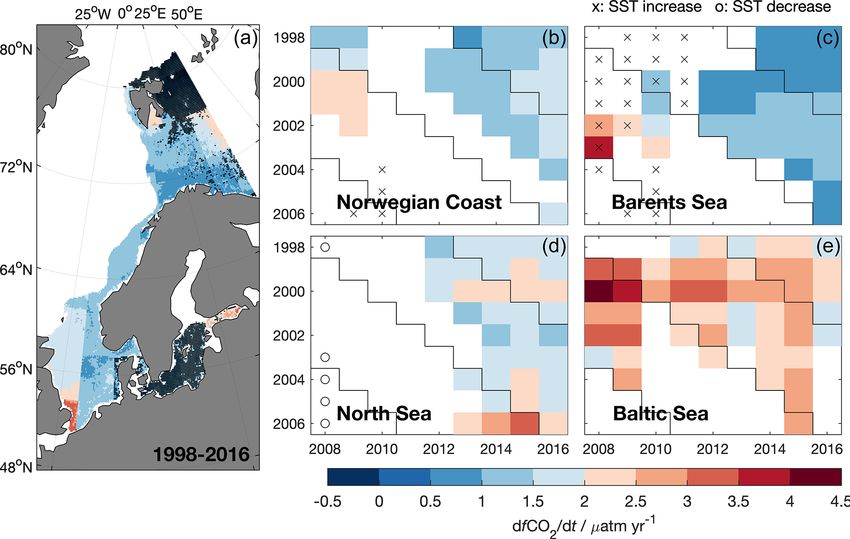
1134                                                                                     M. Becker et al.: Coastal f CO2 maps

inferior to those of MLR 1 (Table 5 and Fig. 3, MLR 3 only),       (2) using the average deviation and its SD, as well as the ME
we will use MLR 1 results for the further analyses. An ex-         between the produced f CO2 maps and the gridded observa-
tended validation of the MLR 1 maps can be found in the            tions as a regional average; (3) showing the median deviation
discussion section.                                                between the MLR and the gridded observations on a monthly
   Figure 4 shows the monthly averages of f CO2 produced           level; and (4) by comparing the data from the f CO2 maps to
by MLR 1 for February, May, August and November. In                observations from two time series stations. (2)–(4) will be
all regions, the highest f CO2 values occur in the winter,         shown for the time period covered by the driver data (1998–
while the lowest f CO2 values occur in summer. The largest         2016) and for the prediction of the f CO2 values for 2017
seasonal cycle could be observed in the Baltic Sea, where          and 2018. These predicted values are compared with data
f CO2 reached well below 200 µatm in midsummer and over            from the newest SOCAT release (SOCATv2019) and provide
500 µatm during the winter.                                        a comparison with an independent dataset. Please note that
   We notice that the gradients that exist between the grid        the comparability of the model performance between the dif-
cells in the Rödenbeck map are still visible in our maps in        ferent regions is limited. All statistical parameters used are
some regions, for example the sharp gradient in the south-         influenced by characteristics that can vary substantially be-
ern North Sea in February or the east–west and north–south         tween the different regions, such as range of the data, their
gradients in the entire North Sea in August. Such gradients        variability or the amount of grid cells with data. For exam-
are also evident in directly mapped pCO2 data (Kitidis et al.,     ple, in a diverse region with many measurements the amount
2019); however, here they are strongly meridional and latitu-      of variability captured by these measurements is most likely
dinal in their extent. As such, while these gradients do reflect   larger and thus will lead to a weaker correlation.
actual features of the f CO2 distribution in the North Sea,           Generally, the uncertainty of MLR 1 is in the same range
their specific shape here is also a consequence of the influ-      as in other studies (Laruelle et al., 2017; Yasunaka et al.,
ence of the Rödenbeck maps on our estimates – from the use         2018) mapping coastal f CO2 dynamics: 25 µatm in the
of these maps as a driver in the MLR and their importance in       North Sea, 16 µatm along the Norwegian Coast, 12 µatm in
improving the statistical performance vs. the MLR that did         the Barents Sea and 39 µatm in the Baltic Sea (based on
not use these values as a driver (MLR 1 vs. MLR 3, Table 5).       the RMSE in Table 5). In the Baltic Sea, which has a large
Also, they do reflect the uncertainty of – and our level of        variability in itself, Parard et al. (2016) obtained lower SDs
confidence in – the estimated pCO2 values, being approxi-          through dividing the area in smaller sub-regions.
mately similar to or slightly larger than the RMSE of MLR 1           One clear drawback of the here presented MLR 1 is the
(Table 5). Any smoothing would be completely artificial and,       clearly visible grid pattern of the open-ocean pCO2 product
while being more visually pleasing, would not better reflect       that was used as input data with its grid size of 5◦ × 4◦ , men-
the truth in any meaningfully quantifiable extent. We have         tioned in Sect. 3.1. There are two ways how one could get
therefore chosen to leave them untouched. These gradients          rid of this artifact in a future release. A finer resolution of the
are therefore also visible in subsequent pH and trend maps.        open-ocean maps used will lead to a better representation of
                                                                   the actual gradients in our mapped product. Rödenbeck et al.
3.2    Maps of pH                                                  just released a newer, finer resolution of their open-ocean
                                                                   product (2.5◦ × 2◦ ) that we intend to use in a future version
The monthly average of pH calculated from MLR 1 f CO2              of this data product. However, this will not be sufficient to
ranges from about 8 during winter to 8.15 during summer in         eradicate the artifact completely. Another approach, running
the North Sea and at the Norwegian Coast (Fig. 5). Towards         the MLR without an open-ocean pCO2 product, can provide
the Barents Sea the pH maximum during summer increases             a coastal pCO2 product without this artifact. While in prin-
to 8.2. The pH of 8.00–8.15 in regions with a large influence      ciple it is preferential to have coastal maps that are indepen-
from the Atlantic, such as the northern North Sea and the          dent of the open-ocean products, MLR 3, which is running
Norwegian Coast, is in good agreement with the range of pH         without open-ocean pCO2 as a driver, clearly did not reach
determined for the open North Atlantic (Lauvset and Gruber,        the same accuracy as MLR 1 (Table 5). New and better input
2014; Lauvset et al., 2015). In the North Sea, the pH is in the    fields or a different regression method could help improve
same range as reported in Salt et al. (2013), and it also shows    the independent coastal maps in the future. Another impact
the same distribution in August/September, with higher pH          that the open-ocean pCO2 product of Rödenbeck et al. can
in the northern North Sea and lower pH in the southern part.       have on MLR 1 is the potential introduction of patterns from
                                                                   regions further away as the spatial correlations used in pro-
4     Discussion                                                   ducing the Rödenbeck et al. pCO2 just ignore land barriers.
                                                                   However, the influence of these spatial correlations is rela-
4.1    Performance of the pCO2 maps                                tively small in regions with a high data density (as the Eu-
                                                                   ropean shelf) and the multi-linear regression used to produce
The performance of the MLR and the maps is evaluated in            MLR 1 corrects for this.
different ways: (1) using the R 2 and the RMSE of the fit;

Biogeosciences, 18, 1127–1147, 2021                                                    https://doi.org/10.5194/bg-18-1127-2021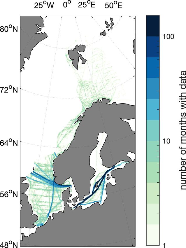
M. Becker et al.: Coastal f CO2 maps                                                                                        1135

Figure 4. The average f CO2 of MLR 1 (1998–2016) for 1 example month in each season (February, May, August and November).

Figure 5. The average pH based on MLR 1 (1998–2016) for 1 example month in each season (February, May, August and November).

   The seasonal differences between MLR 1-determined val-         good agreement in the North Sea (2 ± 20 µatm) and no sea-
ues and the SOCAT v5 data for each region are shown in            sonal bias (Fig. 7). In the other regions, the agreement
Fig. 6. This comparison shows a very good agreement. For          is somewhat reduced compared to the years 1997–2016
MLR 1, the seasonal variations of the median bias are small       (−9 ± 39 µatm (Norwegian Coast), −5 ± 29 µatm (Barents
in the North Sea, along the Norwegian Coast and in the Baltic     Sea) and 28 ± 58 µatm (Baltic Sea)). In these regions we also
Sea. In the Barents Sea, however, the bias varies seasonally.     observe a seasonal bias in the years 2017 and 2018. At least
Here, MLR 1 slightly underestimates the f CO2 in winter and       for the Baltic Sea this could be a result of the extraordinary
early spring, while it overestimates the f CO2 in summer. In      warm and dry summer in 2018 that led to very low f CO2 val-
all other regions, the median seasonal bias is smaller than       ues (see Fig. 8 and the data in SOCAT, Bakker et al., 2016).
the uncertainty of the maps. The larger seasonal bias in the      Please note that for this comparison the MLR was extrapo-
Barents Sea is most likely caused by the larger seasonal bias     lated in time. Only observations until December 2016 were
in the number of available observations. There are no data        used to produce the MLR. Therefore accuracy of the maps
available in October, December and January.                       itself is reduced.
   When comparing all observations from the years 2017               In a second test to investigate to which extent MLR 1 can
and 2018 to the predictions by the MLR 1, we find a               reproduce observations we compared the MLR output with

https://doi.org/10.5194/bg-18-1127-2021                                                  Biogeosciences, 18, 1127–1147, 2021
1136                                                                                         M. Becker et al.: Coastal f CO2 maps

Figure 6. Boxplots showing the median deviation of MLR 1 from the gridded SOCAT 5 data for each region (red line). The boxes show the
upper and lower 75th percentiles. Ninety-nine percent of the data lie within the range of the purple whiskers. Extremes are shown as gray
crosses.

time series data from two voluntary observing ship lines in            occur in the northeastern Barents Sea as well as in parts of
two very different regions with a good data coverage: M/V              the Baltic Sea (about 0.01 % of the grid cells in each region).
Nuka Arctica in the northern North Sea (0–2◦ E, 58–60◦ N)              As pH cannot be calculated for negative f CO2 , we excluded
and M/V Finnmaid in the Baltic Sea (23–24◦ E, 59–60◦ N)                all negative f CO2 values for the calculation of pH. Exclud-
(Fig. 8). The agreement between the MLR 1 and the obser-               ing the negative values resulted in a change in the average
vations is very good. MLR 1 reproduces the general season-             f CO2 of 0.05 µatm (Baltic Sea) and 0.3 µatm (Barents Sea)
ality and some of the interannual variability, also in the years       so they are of negligible importance for the flux estimates.
2017 and 2018, the observations of which were not used in              While the negative values are easy to spot and discard, there
the regression.                                                        are most likely other unrealistically low values in spring and
   When performing interpolation exercises it is always im-            summer in the very north and northeastern Barents Sea as
portant to be aware of the fact that the resulting maps might          well as some parts of the Baltic Sea. However, there are no
come with biases and do not represent all regions equally              data available in SOCAT v5 or available elsewhere to vali-
well. While the here presented maps give a good general                date this.
overview about the surface ocean f CO2 variability in re-                 All regions with questionable f CO2 are also questionable
gions with a relatively large amount of data, the reliabil-            in their pH data. There is a number of very high pH regions
ity, however, is limited in regions where the data coverage            in the Barents Sea (Fig. 5) that are associated with also very
is more scarce. This is especially the case when the region            low f CO2 (Fig. 4) that might not be realistic. In addition,
with scarce data coverage is showing different characteris-            estimated pH values in low-salinity regions where the actual
tics in, for example, temperature and salinity, compared to            alkalinity–salinity deviates strongly from the Nondal et al.
the rest of the region. One such example is the Gulf of Both-          (2009) one used here (e.g., river mouths in the southern North
nia in the Baltic Sea region where almost all data used to             Sea or the Skagerrak) should be interpreted with caution.
derive the MLR is from south of 60◦ N, i.e., not in the Gulf
of Bothnia but in the Baltic Proper and western Baltic Sea
(see Fig. 2). The MLR method can also lead to unrealistic
extreme values and even negative f CO2 . Some such values

Biogeosciences, 18, 1127–1147, 2021                                                       https://doi.org/10.5194/bg-18-1127-2021
M. Becker et al.: Coastal f CO2 maps                                                                                                 1137

Figure 7. Boxplots showing the median deviation between MLR 1 (based on observations until 2016) and measured f CO2 values in 2017
and 2018. The boxes show the upper and lower 75th percentiles. Ninety-nine percent of the data lie within the range of the purple whiskers.
Extremes are shown as gray crosses. The numbers of grid cells with data available were 5047 for the North Sea, 1543 for the Norwegian
Coast, 2312 for the Barents Sea and 5414 for the Baltic Sea.

Figure 8. Time series of ship-of-opportunity (SOOP) data from Nuka Arctica (a, blue) and Finnmaid (b, blue) compared with MLR 1 at the
same location (red). In light blue the predictive MLR output for the years 2017 and 2018 is shown.

https://doi.org/10.5194/bg-18-1127-2021                                                         Biogeosciences, 18, 1127–1147, 2021
1138                                                                                       M. Becker et al.: Coastal f CO2 maps

4.2    Trends in f CO2 and pH                                       Table 6. f CO2 trend calculated from gridded, deseasonalized SO-
                                                                    CAT v5 observations.
Trends in surface ocean f CO2 in coastal regions are often
difficult to assess because of the scarcity of data relative to      Region                     Latitude (◦ N)   Trend (µatm yr−1 )
the highly dynamical character of these regimes and their            North Sea, south                51–54.5              3.2 ± 1.3
large interannual variability. For example, the start of the pro-    North Sea, center               54.5–58           1.43 ± 0.21
ductive season can range from February to April even within          North Sea, north                  58–62         2.320 ± 0.089
a small area, such that even restricting the analysis to specific
                                                                     Norwegian Coast, south            62–68           2.12 ± 0.19
seasons (e.g., winter) can be challenging. Also, due to a lack       Norwegian Coast, north            68–73         1.426 ± 0.099
of data, especially winter data, most observational studies are
based on summer data. Further, the fact that these measure-          Barents Sea, south                69–74           1.31 ± 0.30
ments typically do not take place every year adds even more          Barents Sea, north                74–85           1.01 ± 0.22
uncertainty to the estimated trend, as interannual variability       Baltic Sea, south                 54–56           2.05 ± 0.12
can mask the trend signal.                                           Baltic Sea, north                 56–61           1.84 ± 0.21
   The monthly maps of f CO2 from 1998 to 2016 enable us
now to estimate the trend in surface ocean f CO2 for the en-
tire region, equally distributed over the seasons (Fig. 9, left).
All trends were computed from deseasonalized data. The in-          were covering periods shorter than 10 years (Table 1). In or-
terannual variability of the trend estimates in each region is      der to compare the general patterns of f CO2 trends deter-
shown in the panels on the right hand side in Fig. 9. We ex-        mined from our maps with those directly determined from
clude the northern Baltic Sea from the trend map because we         observations over a similar time range, we estimated the
do not expect to have a robust trend estimate in that region as     f CO2 trends also from the SOCAT v5 observations that were
there are only very few data from that region in the regres-        used to produce the MLR (Table 6). We gridded and desea-
sion. Based on the linear regression the significant trends in      sonalized the SOCAT v5 data and divided the entire region
f CO2 have an average uncertainty of 0.5 µatm yr−1 (North           into nine subregions. A figure showing the fits and the data
Sea), 0.4 µatm yr−1 (Norwegian Coast), 0.4 µatm yr−1 (Bar-          coverage can be found in Appendix A. These observation-
ents Sea) and 0.7 µatm yr−1 (Baltic Sea), while the shorter         based trends show similar general patterns as those based on
time periods shown have a higher uncertainty; no time peri-         our maps (Fig. 9, 1998–2016): (1) largest trends in the south-
ods longer than 1998–2016 (for which the given uncertain-           ern North Sea, (2) decreasing towards the north with trends
ties of the trend apply) are shown. For pH trends, the av-          around the atmospheric trend in the northern North Sea and
erage uncertainties of the regressions over 1998–2016 are           trends around 1 µatm yr−1 in the Barents Sea, and (3) close
5 × 10⁻⁴ (North Sea) and 7 × 10⁻⁴ (Norwegian Coast and              to atmospheric trends in the Baltic Sea.
Barents Sea).                                                          The observation that some subareas (the Baltic Sea or
   In most of the regions addressed in this study, the trend        along the shore of the western North Sea) did not show a
in the surface ocean is lower than the trend in atmospheric         significant trend can be explained by the fact that coastal sea
xCO2 (global average 2.02 ppm yr−1 (Cooperative Global              systems, especially enclosed areas such as the Baltic Sea, ex-
Atmospheric Data Integration Project, 2015)). Trends ex-            perience a high anthropogenic pressure. Anthropogenic im-
ceeding the atmospheric values in the period from 1998 to           pacts other than rising atmospheric CO2 concentrations influ-
2016 can only be observed at the entrance of the English            ence the ocean carbon system; for example the nutrient load
Channel, in Storfjorden/Svalbard and the Gulf of Finland            of rivers can affect coastal ecosystems and primary produc-
(2.5–3 µatm yr−1 ). It has to be noted that there was almost        tion through eutrophication. This will result in lower f CO2
no measured f CO2 as MLR input from Storfjorden. There-             in summer and higher f CO2 in winter (Borges and Gypens,
fore, these trends are highly uncertain. The trend in the west-     2010; Cai et al., 2011). Another important process that in-
ern North Sea is only slightly lower than the trend in the at-      fluences the carbon system in the Baltic Sea is inflow events
mosphere (1.5–2 µatm yr−1 ), while the trends in the eastern        from the North Sea. In between such events, CO2 accumu-
North Sea, along the Norwegian Coast and in the Barents             lates in deeper water layers, causing an increasing gradient
Sea are lower (0.5–1.5 µatm yr−1 ). In the North Sea this is        of dissolved inorganic carbon (DIC) across the halocline.
consistent with a recent study of Omar et al. (2019), which is      Whenever deep winter mixing occurs, this will then lead to
directly based on observations. These low trends will result        a large increase in surface f CO2 because of the input of
in an increase in the strength of the ocean carbon sink with        DIC-rich waters from below. Another reason is the observed
time.                                                               change in alkalinity with time. This affects the f CO2 though
   Generally, only few regressions over time ranges of less         changes in the buffer capacity of the inorganic carbon system
than 10 years turned out to be significant. This is an impor-       (Müller et al., 2016).
tant finding when comparing the trends determined from our             In most other regions, the sea surface f CO2 trends were
maps with the trends reported in literature, many of which          typically smaller than the rise in the atmospheric CO2 con-

Biogeosciences, 18, 1127–1147, 2021                                                      https://doi.org/10.5194/bg-18-1127-2021
M. Becker et al.: Coastal f CO2 maps 1139 Figure 9. The trend in surface ocean f CO2 estimated from deseasonalized f CO2 . Panel (a) shows the spatial distribution of the trend over the time period from 1998 to 2016. Grid boxes without a significant trend are denoted with a black dot. Panels (b)–(e) show the trends in different time periods in four regions, from the various years on the y axis to the various years on the x axis. Non-significant trends were left blank. Significant trends in sea surface temperature are indicated with crosses/circles. The color bar is centered on the approximate annual f CO2 rise in the atmosphere (2 µatm yr−1 ). Figure 10. (a) The long-term trend (1998–2016) in surface ocean f CO2 each month. (b) The average seasonality in f CO2 for the periods 1998–2007 (green) and 2007–2016 (purple) in the northeastern North Sea (58–60◦ N, 3–8◦ E), normalized to December. The SD for each month is shown as the shaded area. centration. A possible explanation is an earlier onset of the et al., 2006). The bloom timing and onset were found to be spring bloom. For example, in the North Sea a significant significantly earlier in the 2010s compared to the previous drawdown in f CO2 has been observed as early as Febru- decades (Desmit et al., 2020). Even if the trend in winter ary in some years, but there is also a large variability (Omar f CO2 was following the atmospheric xCO2 increase, such et al., 2019). The bloom timing and onset in the North Sea a change in bloom timing and onset would lead to a trend after the 1990s have been shown to be mainly triggered by lower than in the atmosphere when averaging over the en- the spring–neap tidal cycle and the air temperature (Sharples tire year. Figure 10a shows the annual trends in f CO2 in https://doi.org/10.5194/bg-18-1127-2021 Biogeosciences, 18, 1127–1147, 2021
1140 M. Becker et al.: Coastal f CO2 maps
each month in the four regions considered. Particularly in 4.3 CO2 disequilibrium and flux
the North Sea and Baltic Sea, very low f CO2 trends are ob-
served in February–May, suggesting that changing timing of The average air–sea CO2 disequilibrium
the spring bloom might be important here. Investigating the (1f CO2 = f CO2,sea − f CO2,atm ) is shown in Fig. 12.
seasonal f CO2 in more detail (Fig. 10b) revealed an ear- The only region showing an average supersaturation is the
lier and deeper f CO2 drawdown in the second decade of southern North Sea. Towards the north, the surface ocean
our analysis (2007–2016) than in the first (1998–2007) in becomes more and more undersaturated, with the lowest
the northeastern North Sea (58–60◦ N, 3–8◦ E). This strongly values in the Barents Sea. The values in the Barents Sea
suggest that an earlier and stronger spring bloom is lower- (−60 to −80 µatm in the southern Barents Sea and less than
ing the annual f CO2 growth rates in this region, which is −100 µatm around Svalbard) are in agreement with those
among the ones with the smallest f CO2 trends in the North estimated by Yasunaka et al. (2018). The seasonal cycle of
Sea (about 1 µatm yr−1 , Fig. 9). In the other regions, no such 1f CO2 follows a biologically driven pattern with higher
changes could be established with confidence. Future inves- values in the winter and lower values from April to August.
tigations should aim at generating f CO2 maps with higher The seasonal cycle is largest in the Baltic and smallest in the
temporal resolution, as changes in the timing of the spring Barents Sea.
bloom might be a matter of days or weeks, which would not The air–sea CO2 fluxes and their trends (Fig. 13) show
be fully resolved by the monthly maps presented here. that most regions are a net and increasing sink for CO2 . The
When looking at the interannual variability, it becomes only net source regions are the southern North Sea and the
obvious that the trend in the North Sea is slightly smaller Baltic Sea. The two different regimes in the North Sea, with
than the atmospheric CO2 trend. In contrast, the Norwe- the southern, nonstratified part being a source and the north-
gian Coast and the Barents Sea experience a robust trend ern temporarily stratified part a sink for CO2 , have been de-
much lower than the atmospheric trend (Norwegian Coast: scribed in the literature before (Thomas et al., 2004), but
1–1.5 µatm yr−1 ; Barents Sea: around 1 µatm yr−1 ). Here we the gradient between them as represented here may be a too
can also see a stable pattern of warming over timescales of sharp (Sect. 3.1). However, there is a large interannual vari-
10 to 15 years. The warming in itself would result in an in- ability in the f CO2 disequilibrium (Omar et al., 2010), and
crease in f CO2 with time, in addition to the atmospheric studies based on different years find conflicting results re-
forcing. As we are observing a trend smaller than the at- garding the direction of the flux (Kitidis et al., 2019; Schiet-
mospheric trend, temperature effects cannot be the driver tecatte et al., 2007; Thomas et al., 2004). This large interan-
here. The lower trend stems most likely from an earlier onset nual variability was also present in our maps. During some
of spring bloom. It has been shown that the Atlantification years, larger parts of the North Sea were a net source, while
and the reduced ice coverage of the Barents Sea lead to a during other years also the southern North Sea acted as net
longer productive season, and this will result in more months sink (not shown).
with strong undersaturation in CO2 (Oziel et al., 2017). In The seasonal variations in the air–sea flux are driven by a
the Baltic Sea the patterns are different. Here the variabil- combination of the changes in the disequilibrium, the wind
ity is much larger, while most of the time periods show a strength and the ice cover. As there is less wind during sum-
trend larger than the atmospheric trend (3–3.5 µatm yr−1 ). mer, when the disequilibrium is large, but a smaller disequi-
Although slightly smaller our results broadly agree with librium during winter, when the wind strength is high, the
trend estimates based on measurements of 4.6–6.1 µatm yr−1 seasonal variability in the flux is often less clear than that in
over 2008–2015 (Schneider and Müller, 2018). Finally, it the disequilibrium. This can be seen in the Barents Sea and
also needs to be noted that the uncertainty of the f CO2 maps Norwegian Coast. Yasunaka et al. (2018) found the seasonal
was highest in the Baltic Sea. This makes it also more diffi- and interannual variation in the Barents Sea and the Norwe-
cult, if not impossible, to properly detect these small differ- gian Sea mostly corresponded to the wind speed and the sea
ences in the trends. ice concentration. We see the strongest dependence on the
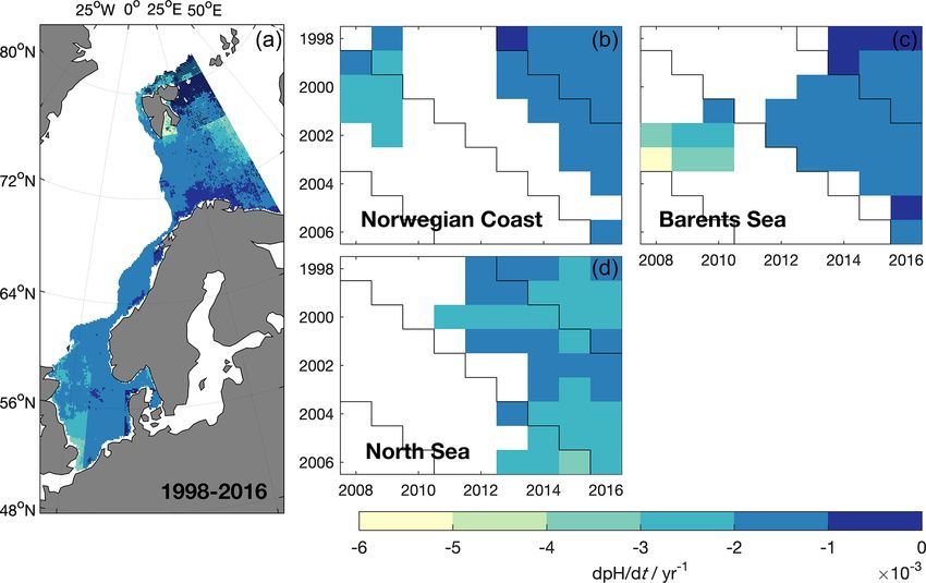
For pH, the trend in most regions is around −0.002 yr−1 air–sea disequilibrium, however (not shown). This indicates
(Fig. 11). As expected, regions with the strongest trend in that the seasonal and interannual variability in our f CO2
f CO2 also show the highest trend in pH, such as the south- maps is larger than in the maps generated by Yasunaka et al.
ern North Sea. The trend in the northern North Sea and (2018). Still, our average fluxes fit well with those reported
along the Norwegian Coast is in good agreement with the pH by Yasunaka et al. (2018) of −8 to −12 mmol m−2 d−1 (Bar-
trends found in studies focusing on the open Atlantic Ocean ents Sea) and −4 to −8 mmol m−2 d−1 (Norwegian Coast).
(−0.0022 yr−1 , Lauvset and Gruber, 2014) and the North At- In the North Sea there is almost no net flux during win-
lantic and Nordic Seas (−0.002 yr−1 , Lauvset et al., 2015). ter, as the surface ocean is more or less in equilibrium with
the atmosphere. In the Baltic Sea, there are high fluxes into
the atmosphere during winter as here a large oversaturation
coincides with strong winds. This is also why the Baltic
Sea is a net source region. Although Parard et al. (2017)
Biogeosciences, 18, 1127–1147, 2021 https://doi.org/10.5194/bg-18-1127-2021M. Becker et al.: Coastal f CO2 maps 1141 Figure 11. The trend in surface ocean pH estimated from deseasonalized pH. (a) The spatial distribution of the trend over the time period from 1998 to 2016 is shown. Grid boxes without a significant trend are denoted with a black dot. Panels (b)–(e) show the trends in different time periods in three regions, from the various years on the y axis to the various years on the x axis. Non-significant trends were left blank. Figure 12. The average air–sea CO2 disequilibrium over the period 1998–2016 (a, red colors indicate average undersaturation, while blue colors indicate average oversaturation). For every region average disequilibria are shown as seasonal averages (b) and time series of annual disequilibria (c). Blue line: North Sea; red line: Norwegian Coast; yellow line: Barents Sea; purple line: Baltic Sea did find slightly smaller seasonal fluxes (+15 mmol m−2 d−1 uncertainty of the 1f CO2 is mostly driven by the uncer- during winter and −8 mmol m−2 d−1 during summer), the tainty of the MLR, resulting in an error between 12 and annual air–sea CO2 fluxes are in good agreement (0 to 39 µatm, according to the RMSE values of MLR1 for the +4 mmol m−2 d−1 between 1998 and 2011). different regions (Table 5). A number of studies address the The uncertainty in the calculated fluxes is a result of the uncertainty of gas exchange parameterizations and the wind uncertainties in the f CO2 observations, 1f CO2 maps, the products (Couldrey et al., 2016; Gregg et al., 2014; Ho and gas exchange parameterization and the wind product. The Wanninkhof, 2016). For this study, we apply an uncertainty https://doi.org/10.5194/bg-18-1127-2021 Biogeosciences, 18, 1127–1147, 2021
1142                                                                                         M. Becker et al.: Coastal f CO2 maps

Figure 13. The average air–sea CO2 flux over the period 1998–2016 (a, red colors indicate sink regions, while blue colors indicate source
regions). For every region average fluxes are show as seasonal averages (b) and time series of annual fluxes (c).

of the gas transfer velocity of 20 % (Wanninkhof, 2014).               in regions with only a small number of observations as the
This will result in an uncertainty of the air–sea flux of about        MLR can lead to unrealistic values.
2 mmol C d−1 m−2 . It has to be kept in mind that the absolute            Long-term observations with a high temporal resolution
uncertainty in k increases with increasing wind speed but that         are extremely important for developing maps such as pre-
the uncertainty in the wind speed has the largest influence in         sented here. While a decent spatial coverage exists for the
summer when also the disequilibrium is large. In contrast,             open North Atlantic, most coastal regions are still undersam-
the uncertainty in 1f CO2 will cause larger errors in winter,          pled, in particular relative to their high variability in time and
when the wind speeds are high.                                         space. To further understand and interpret the trends in f CO2
   There is an ongoing discussion of how and to which extent           and pH it is necessary to increase our knowledge and under-
the dominant climate mode in the North Atlantic, the North             standing of the interaction between primary production, res-
Atlantic Oscillation (NAO), is driving the variability in the          piration in the water column and the sediments, mixing and
CO2 fluxes (Salt et al., 2013; Tjiputra et al., 2012; Watson           gas exchange, and their influence on the carbon cycle.
et al., 2009). Even though some features in the time series               Besides an increased amount of in situ observations, also
seem to coincide with very extreme states of the NAO, such             improved, higher-resolution driver data hold the potential to
as a very large disequilibrium along the Norwegian Coast in            enable a better representation of spatial gradients. Including
2010, we could not find any significant correlation between            not only satellite-derived chlorophyll data but also colored
the CO2 fluxes and the NAO index.                                      dissolved organic matter (CDOM) can also lead to an im-
                                                                       proved performance of the regressions, especially in regions
                                                                       with a high load of terrestrial dissolved organic carbon.
5   Conclusions                                                           While MLR-derived sea surface f CO2 maps provide a co-
                                                                       herent picture of the entire region, they have clear limitations
The MLR approach presented in this work is a relatively easy           and should be interpreted with caution in regions with few or
and straight forward method to produce monthly f CO2 maps              no observations. A large number of observations is essential
with a high spatial resolution in coastal seas, and the use of         both for producing high quality maps and for their validation.
available open-ocean maps improved the coastal maps sig-               Also, observations of a second parameter of the carbon sys-
nificantly. The maps reproduce nicely the main spatial and             tem would be beneficial for deriving pH maps – to reduce and
temporal patterns that are present in observations in the dif-         quantify the error introduced by estimating alkalinity from
ferent regions for both f CO2 and pH. The surface seawater             salinity. In addition to that, our work neglects the areas clos-
f CO2 trends were mostly lower than the atmospheric trends             est to land due to unavailability of CO2 data and reanalysis
and also lower than the trends found in the open North At-             products in those areas. For adding their contribution to the
lantic. Results show that the northern European shelf is an in-        flux estimates, new platforms specialized on measurements
creasing net sink for CO2 . Only the Baltic Sea is a net source        directly at the land–ocean interface need to be developed.
region. This method clearly has the potential to be extended
to a larger region. However, it should be handled with care

Biogeosciences, 18, 1127–1147, 2021                                                       https://doi.org/10.5194/bg-18-1127-2021
You can also read