CAST Status Report to the SPSC for the 142nd Meeting

CAST
 Status Report to the SPSC for the 142nd Meeting
CERN-SPSC-2021-017 / SPSC-SR-292

 CERN, May 28, 2021
 29/05/2021

 On behalf of the CAST Collaboration,
 Editor: Horst Fischer
 Albert-Ludwigs-Universität Freiburg
 Physikalisches Institut
 Hermann-Herder-Str. 3
 79104 Freiburg im Brsg.

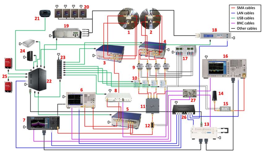
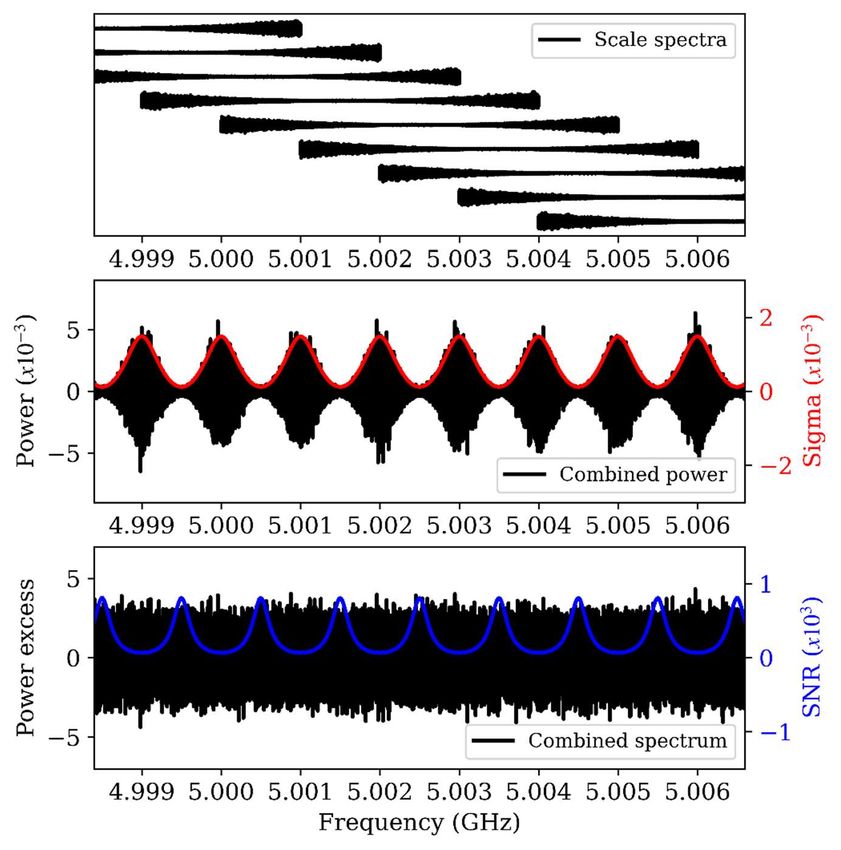
Table of Contents
1 Technical Coordination: Status of CAST Infrastructure.......................................................... 1
 1.1 2020 data taking campaign .................................................................................................. 1
 1.2 2021 data taking campaign .................................................................................................. 1
2 CAST-CAPP – Wide band dark matter axion search .............................................................. 1
 2.1 Summary .............................................................................................................................. 1
 2.2 Data taking campaign 2020/2021 ........................................................................................ 2
 2.2.1 Measurements with single cavities .................................................................................. 2
 2.2.2 Phase Matching ................................................................................................................ 2
 2.3 DAQ system and strategies .................................................................................................. 3
 2.3.1 DAQ chain ....................................................................................................................... 3
 2.3.2 Identifying electromagnetic interferences ........................................................................ 5
 2.3.3 Signal injections ............................................................................................................... 6
 2.3.4 Fast Resonant Frequency Tuning..................................................................................... 7
 2.4 Data Analysis ....................................................................................................................... 7
 2.4.1 Parameters optimization................................................................................................... 7
 2.4.2 Noise distribution cross-checks ..................................................................................... 10
 2.4.3 Quality checks ................................................................................................................ 11
 2.4.4 Results and outliers ........................................................................................................ 11
 2.5 Future Prospects ................................................................................................................. 12
 2.6 Concluding Remark ........................................................................................................... 13
3 RADES – High-mass axion search ........................................................................................ 19
 3.1 Developments since October 2020 .................................................................................... 19
 3.1.1 Submission of 2018 data-taking results for publication................................................. 19
 3.1.2 Data-taking 2020-2021 .................................................................................................. 19
 3.2 Future possibilities for RADES in CAST .......................................................................... 20
4 The new solar axion data taking campaign with the IAXO pathfinder system at CAST ...... 20
 4.1 Summary and goals ............................................................................................................ 20
 4.2 Preliminary considerations ................................................................................................. 21
 4.3 Status and achievements .................................................................................................... 21
 4.4 Data taking campaign with Xe-based mixtures ................................................................. 21
 4.5 Data analysis ...................................................................................................................... 22
 4.6 Preliminary background spectrum with Xenon ................................................................. 23
 4.7 Low gain runs..................................................................................................................... 23
5 InGrid/GridPix detector – Search for low energy solar ALPS .............................................. 24
 5.1 Stability of energy calibration ............................................................................................ 24
 5.2 Optimization of energy-dependent likelihood selection .................................................... 25
 5.3 Advancement towards more modern statistical interpretation (profile likelihood) ........... 25
 5.4 Further improvements ........................................................................................................ 26
6 KWISP – Chameleon Search with an opto-mechanical detector ........................................... 26
 6.1 Introduction ........................................................................................................................ 26
 6.2 KWISP 3.5 set-up .............................................................................................................. 26
 6.3 Recent upgrades ................................................................................................................. 27
 6.4 Data taking ......................................................................................................................... 28
 6.5 Results ................................................................................................................................ 28
 6.6 Conclusions ........................................................................................................................ 30

1 Technical Coordination: Status of CAST Infrastructure

1.1 2020 data taking campaign
In 2020 the magnet was on for a total of 2635 hours. In particular, between the 24th of September
and the 16th of December 2020 the magnet was on for 1277 hours and, parasitically, we followed the
sun during 51 hours without interfering with the DM axion search.

1.2 2021 data taking campaign
In early 2021 it was foreseen that the magnet would be cooled down immediately after the Christmas
break as no mechanical or vacuum interventions were foreseen. In the beginning of 2021 we per-
formed a network upgrade which considerably increased the data transfer speed and we also migrated
from CASTOR data archiving to CTA, but this run in parallel with the CAST planning.
In the beginning of 2021 it was reported that the piezo mechanism of one of the CAPP cavities was
not responding. In an attempt to restore its functionality, on the 7th of January we started actively
warming up the magnet, which was passively warming up since the 16th of December. Until the 17th
of January when we reached almost 295 K, the piezo was not restored. We then started cooling down
on the 18th of January. After the quench training, the magnet was ramped up for the first time for
physics data taking campaign on the 28th of January 2021.
The 2021 data taking campaign was relatively uneventful. We have had two quenches, a natural one
on the 7th of February and one on the 16th of March. The latter was caused by power tests on the
LHC magnets at P8 which caused an overload of 400V consumption on the ERD1 / 8R and ERD2 /
8R panels. The HV protection relay measured this overload and tripped causing the quench.
In total (until 18/5/2021) the magnet was on for 2509 hours. We did 56 solar tracking and the magnet
followed the sun for 84 hours. The data taking hours per detector and the issues of each detector
system will be detailed in the corresponding chapters.

2 CAST-CAPP – Wide band dark matter axion search

2.1 Summary
The CAST-CAPP sub-detector is using 4 microwave cavities searching for Dark Matter axions thus
transforming the CAST experiment from an axion helioscope to an axion haloscope. During the last
months, CAST-CAPP improved its statistical sensitivity having now in total ~153 days of data with
magnetic field ON and focused on the analysis of the data. These soon-to-be-published data in the
range 19.7 to 22.4 μeV (4.7 to 5.5 GHz) allow for a significant increase in sensitivity, exceeding
previous measurements by almost two orders of magnitude. The upgrade of the DAQ chain and the
progress in the analysis were crucial to gain a rejection power against electromagnetic parasites.
CAST-CAPP has pioneered a new technology and data-taking strategy, in addition to halo dark matter
axions, through fast resonance scanning and phase-matching of multiple cavities that allows to search
also for transient events. Furthermore, the experience gained with phase matching allows to project
applications in future large scale axion haloscopes like that of the IAXO project.
An extension of the data taking time will allow CAST-CAPP to improve its own cutting-edge limits
on the axion-photon coupling for a relatively wide range of axion masses. Envisioning continued
operation for 12 months of data taking, the sensitivity will reach into the band of theoretical predic-
tions in a yet unexplored mass range.
 1

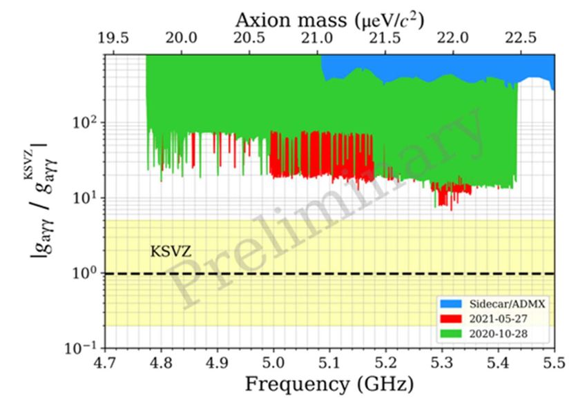
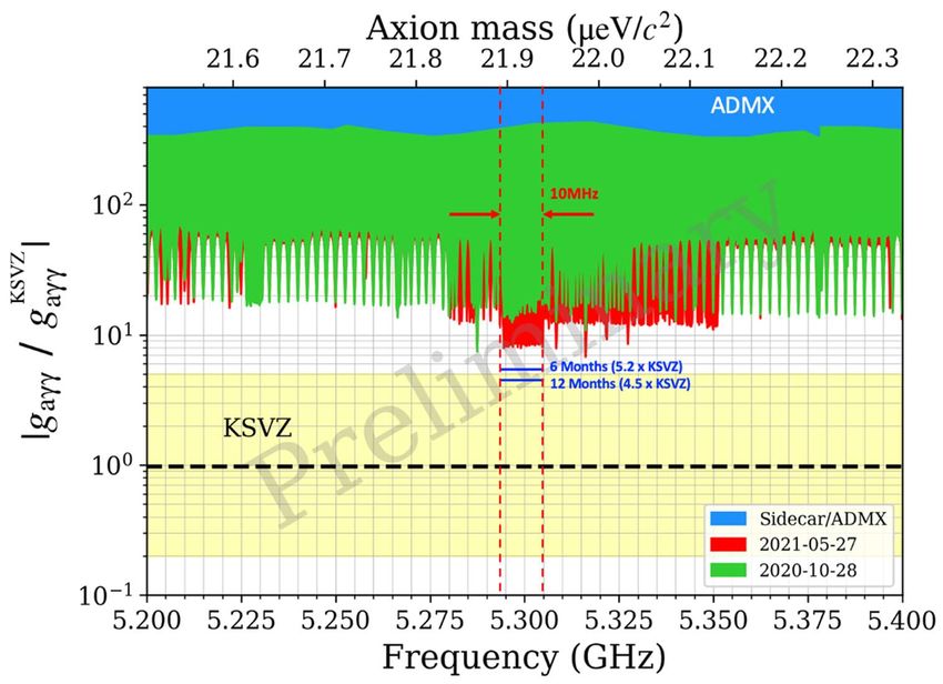
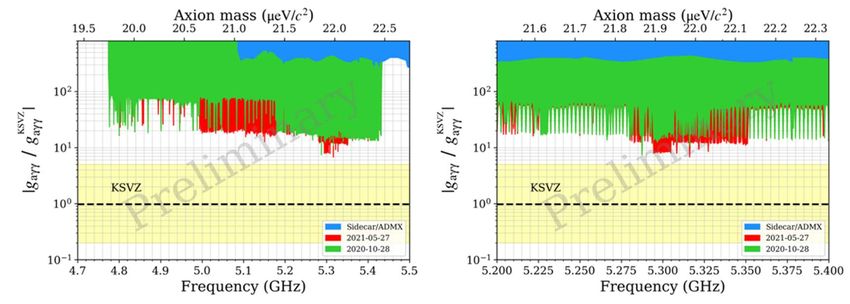
2.2 Data taking campaign 2020/2021
Since the presentation to the SPSC committee (13/10/2020), the CAST-CAPP sub-detector has taken
data in the periods from 23/11/2020 to 16/12/2020 and continuously since 02/02/2021 until today.
The current total acquired data up to 26/05/2021 correspond to 3670.3 hours (152.9 days) for ~ 660
MHz range. This corresponds to a duty cycle of about 16.2 hours/day for the latest runs, with 20
hours/day being the maximum possible rate. The covered frequency range with all cavities is 660.15
MHz from 4.7739 GHz to 5.4341GHz.

2.2.1 Measurements with single cavities
The data-taking time using CAST-CAPP cavities individually is 2126.6 hours (86.6 days). The fre-
quency ranges accessible by the individual CAST-CAPP cavities are:
 ● Cavity 1: 127.6MHz (5.2224 GHz – 5.3500 GHz)
 ● Cavity 2: 199.0MHz (5.1823 GHz – 5.3813 GHz)
 ● Cavity 3: 211.7MHz (5.2224 GHz – 5.4341 GHz)
 ● Cavity 4: 471.9MHz (4.7740 GHz – 5.2459 GHz)
Please note, single manual intervention to the locomotive gear drive enables the scanning of a fre-
quency range extended by a factor of two.

2.2.2 Phase Matching
To increase the effective volume of the CAST-CAPP detector, and therefore its sensitivity, multiple
cavities instead of enlarging a single cavity are used. Further enhancement of the signal-to-noise ratio
(SNR) is made through the “phase matching” technique by combining coherently the power outputs
of each frequency-matched cavity after individual signal amplification. The improvement of SNR
with this method goes linearly with the number of cavities:

 = ∙ 

This technically challenging concept has for the first time been achieved in CAST-CAPP with all
four cavities in a coherent data-taking mode by adjusting the frequency of the cavities within 10kHz
(see Figure 3 in [7]). At the same time to fulfil all the required conditions for optimum phase match-
ing, the electrical length of the output signals, as well as the amplitude of the individual cavities, were
adjusted accordingly. The phase matching concept is also important for scaled-up haloscopes a la
Sikivie, e.g. the IAXO project, as it allows the coherent combination of a large number of cavities up
to the order of 1000 relatively small cavities. Notably, small cavities are necessary to have resonance
conditions for axions above ~10-20 μeV.

The total data-taking time taken so far with phase-matching corresponds to 1543.7 hours (64.3 days)
for a total frequency range of about 205.3 MHz from 5.1482 GHz to 5.3535 GHz. Combining phase-
matched data as well as data from single cavities a competitive limit on the axion-photon coupling
constant has been set (see Figure 2.1). The progress since the last annual SPSC meeting in October
2020 is apparent. In Figure 2.2 an extended frequency range shows the current results compared to
the rest of the experiments. An overview of the analysis steps for deriving these plots is presented in
Section 2.4 “Data Analysis” as well as in the supplement material in Appendix A at the end of chapter
2.

 2

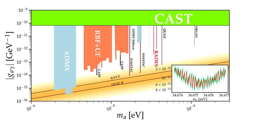
Figure 2.1: Exclusion plot comparison in the full frequency range (left) and around 5.3 GHz (right) assum-
ing galactic halo DM axions from 10/2020 (1461 hours) and 05/2021 (3670 hours). The observed spikes cor-
 respond to longer measurement times at the specific frequencies. For comparison, the ADMX-Sidecar limit
 [2] is also given for galactic axions.

Figure 2.2: Exclusion limits by various experiments on the axion-photon coupling as a function of axion rest
 mass. In the red the latest CAST-CAPP results with a 90% confidence level.

2.3 DAQ system and strategies

2.3.1 DAQ chain
The whole DAQ system has been further improved considerably in both hardware (Figure 2.3) and
software to provide even more functionalities for a more complete insight on the system characteris-
tics allowing for a much faster and user-independent data acquisition procedure as well as faster daily
processing and analysis.

 3

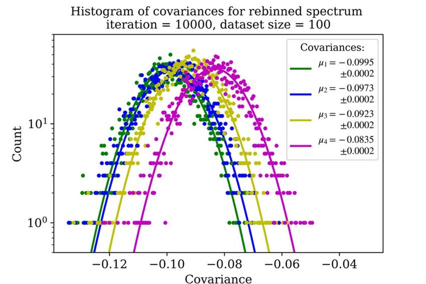
Figure 2.3: Latest CAST-CAPP hardware schematic outside-the-cryostat.

The implementation of a second measuring channel for continuous and simultaneous monitoring of
ambient EMI/EMC parasites (instruments 14-16 in Figure 2.3) including all the necessary upgrades
in the IQC data recorder (instrument 13) was successfully achieved (see also Section 2.3.2). The
simultaneous recording from both spectrum analyzers (instruments 7 and 16) results in a doubling of
the data to 3 GB per 1-min measurement. To mitigate the increased offloading, uploading to CAS-
TOR, and processing times, a few upgrades have been performed:
 ● The IQC data recorder (instrument 13) storage was upgraded from 2 TB to 4 TB RAIDs.
 ● The local pc storage was upgraded from external HDD to 2 x internal SSD drives which were
 RAID together (instruments 25). This increased substantially the read/write speed while of-
 floading and processing the raw data from 130 MB/s to 940 MB/s.
 ● The whole CAST network infrastructure as well as the workstation pc network card were
 upgraded from 1 GB/s to 10 GB/s. In practice, this increased the upload speed to the CASTOR
 tape system by about 5 times.
 ● The multi-threading technique was implemented in processing procedures to allow for simul-
 taneous usage of 6 / 8 cores of the local workstation PC. This allowed simultaneous processing
 of multiple raw data files increasing the processing speed by about 4 times.
Additionally, a 10 MHz reference cable was connected to all new instruments through a power splitter
(instrument 27) to phase lock all the various instruments and allow for higher frequency accuracy.
Regarding offline tape storage, the CASTOR tape system of CERN is currently being replaced by
CTA (CERN Tape Archive) system. Therefore, the migration of all the data from the old system to
the new one took place in January/February 2021. All the submission scripts and the various protocols
for the upload of the CAPP data to CTA through FTS were adjusted accordingly. In addition, new re-
submission automatic procedures were created that allow for a direct upload of all the failed files
which strongly reduces the re-submission times from about 5 hours to 30 min. It is noted that due to
the size of the recorded files there are about 4 TB of data being uploaded daily to CTA which in turn
increases the possibility of files failing. Finally, streaming of the small files below 10 MB that are
uploaded on CTA through an independent protocol allows a much faster upload time for the processed
and analyzed data reducing the time from 1.5 hours to about 8 min.

 4

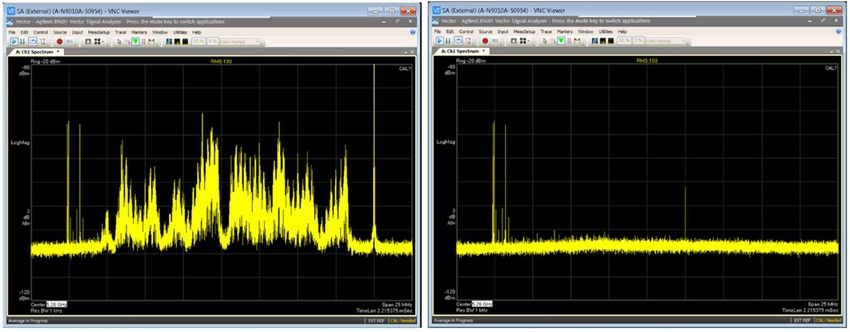
2.3.2 Identifying electromagnetic interferences
The observation of several unintended and intended emitters in the CAST area, operating in our fre-
quency range initiated a wide-search operation for the identification and characterization of these
frequencies. Even though the magnetic body of CAST acts as a Faraday cage shielding the cavities
from outside RF leakages, a small number of strong parasites, about 30 dB above the noise floor, can
make their way in the DAQ chain through outside-the-cryostat connections, amplifiers cables, etc.
Therefore, after the initial manual identification of the frequency, shape, and power of the EMI/EMC
parasite signals in the CAST area, a witness channel has been installed in the DAQ chain on
18/11/2020 for automatic measurement of all these parasitic signals. This independent simultaneous
measuring system performs identification of EMI/EMC parasite signals present in the CAST hall
through a spectrum analyzer connected to an external omnidirectional antenna (instruments 14-16 in
Figure 2.3). This works as a “veto counter” operating at the same band as the cavity measuring chan-
nel constitutes an important upgrade for signal identification which allows for an easier and faster
first characterization of possible outliers (see Figure 2.4). The total exposure time since the initial
installation is about 2139.9 hours (89.2 days).
It is mentioned that with the addition of this EMI/EMC measuring channel and the recent updates in
the analysis procedure, the two spectra from the two simultaneously operated channels can be used
to check daily for short-lived signals that could be associated to transient events. However, ambient
EMI/EMC leaves similar large signatures in the cavity as transient events would do, but can be re-
jected on the basis of simultaneous observation outside the magnetic field (see for example Figure
2.4).

Figure 2.4: Example of an EMI/EMC parasite being present in both cavity measuring channel (upper black spectrum)
 and EMI/EMC measuring channel (lower blue spectrum) at the same frequency.

A significant intended emitter in the CAST hall is the 5 GHz band from WLAN coming from the
Access Points located around the area. After consultation with the responsible CERN WLAN service,
channels 52-56 and 116-120 interfering with our frequency band have been disabled with the
achieved huge suppression being obvious around the related frequencies shown in Figure 2.5.

 5

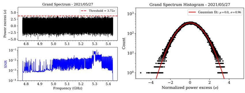
Figure 2.5: Power as a function of frequency, from 5.25 GHz to 5.29 GHz, for the 52-56 WLAN 5GHz chan-
 nels emitting in the CAST area before (left) and after (right) they have been disabled.

2.3.3 Signal injections
Following a suggestion also by the SPSC referees, a new signal generator has been permanently in-
stalled in the DAQ chain (instrument 8 in Figure 2.3) to insert a well-defined pilot tone in the cavity
measurements. This makes sure that a fake axion signal will be identified by the analysis procedure,
but also provides useful information on the stability and calibration of the whole data-taking system.
Recently, the implementation of an automatic signal injection procedure has been completed with a
variety of signals with different amplitudes being injected, recorded, and identified by analysis in
several frequencies. An example of such an injection with a 1Hz CW signal and a sweeping 5 kHz
one within 10 msec is shown in Figure 2.6.

Figure 2.6: Injected signal of -110 dBm power on a cavity with a CW pulse (left column) and -90 dBm with a
5 kHz width (right column). The combination of 12 5-sec traces in a 1-min trace (upper row), as well as the
time evolution (lower row), is showing the amplification of the signal as more and more data are combined,
 thus confirming the analysis procedure.

 6

In addition, in a simulation an axion signal has also been generated and artificially injected into the
raw data. With this simulation, the observation of such a signal via the analysis procedure is also
cross-checked. In Figure 2.7 a simulated axion signal with a coupling 20 times the KSVZ limit and 7
kHz width has been recovered.

 Figure 2.7: Simulation of 110-min simulated raw data including a 20 x KSVZ axion in combined (left) and
 grand (right) spectra. Effect of the analysis procedure is observed as a signal with higher SNR.

2.3.4 Fast Resonant Frequency Tuning
The design of CAST-CAPP allows to eventually profit from the transient flux enhancement [5] in-
cluding gravitational self-focusing due to the density distribution of the inner Earth [6] giving rise to
an eventually large circadian or peaking modulation (see Figure 1 in [7]). Therefore, in addition to
the search for halo DM axions, CAST-CAPP can investigate possible axion transient events in the
axion mass range ~19.7-22.4 μeV thanks to its “fast resonant scanning technique”. The CAST-CAPP
cavities are tuned relatively fast to take advantage of possible streaming dark matter axions without
losing sensitivity for isotropic DM halo, which was of primary interest during the data-taking period.
So far, a wide axion mass range (~660 MHz) could be scanned within a total time interval of a few
hours to eventually take advantage of transient dark matter [1,5,6]. Here, the concurrent direct com-
parison with a simultaneously measuring second spectrum analyzer channel is in particular important
to identify potential EMC/EMI noise. The analysis of the collected data towards such events is pos-
sible and will be intensified at a later stage.

2.4 Data Analysis
The analysis procedure has been quite improved to match the widely accepted methods followed by
other experiments such as ADMX, HAYSTAC, CAPP-IBS, etc [3-4], but has also been adapted to
the specific experimental conditions of CAST-CAPP. Below the most important new additions since
the last SPSC annual meeting are presented along with the latest results.

2.4.1 Parameters optimization
The basic procedure involves the removal of the noise baseline of the processed spectra with the
Savitzky-Golay (SG) filter (see Figure 2.8). SG filter is based on a moving polynomial fits of order p
in window length W. These parameters, p, and W, have to be adjusted for optimal performance.

 7

Figure 2.8: Processed spectrum and its SG filter (upper). Flattened spectrum (lower) is achieved by dividing
 the processed spectrum by its SG filter and subtracting 1.

SG filter is preferred by the vast majority of the axion community as a smoothing filter due to its
nearly perfect pass-band. Still, the adverse effects of its imperfect stop-band should be accounted for
to prevent analysis performance issues. The effect of imperfect SG filter stop-band performance on
the analysis results are twofold:
● The standard deviation of the grand spectrum bin distribution is lowered by the SG filter-induced
 correlations among adjacent bins.
● Axion signals are attenuated due to imperfect stop-band effects.
To understand and minimize these effects, we optimize SG filter parameters (W,p) and run two sim-
ulations to quantify the two effects listed above. First, to do the parameter optimization, we investi-
gate the transfer functions of the SG filters with varying parameters. Figure 2.9 shows the transfer
functions for 2 parameter sets, namely the currently used W=1000, p=4 (left) versus promising
W=2000, p=2 (right). Yellow (axion domain) and brown (cavity resonance domain) colored bands in
the plots reflect the 2 main criteria of optimization: SG filter should have a low transmission for axion
signal and high transmission for cavity resonance bump. We see that a change of parameters from
(W,p) = (1000,4) to (2000,2) brings -3 dB point of the filter closer to cavity resonance domain keeping
its transmission at constant 0 dB (maximum) and lowers the axion signal transmission from ~-20 dB
to ~-30 dB fulfilling our criteria. We are currently running a new analysis campaign to apply a new
SG filter with these optimized parameters.

 Figure 2.9: Different parameters of SG filter to maximize the noise bump transmission while minimizing the axion
transmission. SG filter transfer function for parameters (W,p)=(1000,4) is shown on the left, and (W,p)=(2000,2) on the
 right.

 8

We selected the promising parameters (W,p)=(2000,2) by investigating the SG transmission as a func-
tion of W for several integer p values as depicted in Figure 2.10. There we selected the (W,p) point
that maximizes cavity transmission (dashed lines) and minimizes the axion transmission (solid lines).

Figure 2.10: Variation of cavity (solid lines) versus noise bump (dashed lines) transmissions as a function of
 SG fit-window length, W, and for several integer polynomial orders, p.

The first of the two simulations is used to quantify the SG filter induced standard deviation reduction
in the grand spectrum. In this simulation, we run 104 experiments, each with 100 simulated processed
spectra made of random noise added on sample noise baselines. We evaluate the covariance of the
nearby bins using the mean of the covariance distributions for n cases where the bin displacement is
varied from 1 to n-1 where n is equal to 28 and 5 for the rebinned and the grand spectra, respectively.
Figure 2.11 shows the results of the simulation for the grand spectrum where the covariance of the
nearby bins is quantified to be -0.0995, -0.0973, -0.0923, -0.0835 with ± 0.0002 uncertainty as bin
spacing is varied from 1 (bins that are just next to each other) to 4. The behavior of decreasing covar-
iance is expected as the bin spacing increases. To test the null hypothesis, we conducted the same
simulation on random noise spectra with a flat baseline without SG filter application and we observed
no correlations among adjacent bins as expected.

Figure 2.11: Results of the simulation to quantify adjacent bin correlations in the grand spectrum due to im-
 perfect stop-band of SG filter.

The analysis with (W,p)=(1000,4) results in a grand spectrum with standard deviation σ=0.74 due to
SG filter complications where the expected number is 1. We use the results of the simulation above
in a feedback loop to correct the weights used in the analysis and the corrected standard deviation
σ=0.96, much closer to our expectation of 1. First indications of the currently undergoing analysis
with (W,p)=(2000,2) show we can achieve σ=~1 after the correction.
 9

The second of the two simulations aims to quantify axion signal attenuation due to imperfect SG filter
stop-band. We simulate 103 experiments with injections of digitally synthetic axion signals in 100
simulated spectra. After analyzing each experiment, we histogram the amplitude of axion signal car-
rying bins and compare the results for the cases where SG is used or not used. Results of this simula-
tion indicate that a prospective axion signal SNR may be attenuated up to ~50% given the SG filter
parameters (W,p)=(1000,4) meaning an attenuation coefficient of η=0.5. Since the exclusion perfor-
mance is proportional to the square root of the SNR, the η=0.5 value indicates a decrease in exclusion
by factor ~0.7. Figure 2.12 shows the histograms of the axion signal carrying simulated bins resulting
from 2 channels of the simulation: with (right) and without (left) SG filter application.

 Figure 2.12: Simulated axion power with (right) and without (left) SG filter.

ADMX and HAYSTAC report η ranging between 0.7-0.9 meaning they can preserve 70% - 90% of
the axion signal. This shows we have room for improvement here as well. First indications of the
currently undergoing analysis with (W,p) = (2000,2) SG parameters show that η will increase to the
region where our competitor experiments operate meaning that we will preserve the SNR of an axion
signal better.

2.4.2 Noise distribution cross-checks
An important check in the quality of the receiver chain is to observe the expected noise properties. In
this case, we want to observe the distribution features of the Johnson-Nyquist (thermal) noise in our
spectra. Many noise distribution histograms that we showed to SPSC so far displayed Gaussian dis-
tribution (that look like a parabola on a logarithmic scale) as dictated by the central limit theorem due
to the massive averaging of many spectra. So, to distinguish the noise characteristics, we should focus
on the non-averaged spectrum. The left plot in Figure 2.13 shows voltage and power distributions of
a raw spectrum aligned well with theoretical expectations of χ and χ2 of 2 degrees of freedom, respec-
tively. We tested the well-known 1/√ factor that explains the decreasing error of the mean as more
and more spectra are averaged As the right plot of Figure 2.14 shows, we observe the expected rela-
tion: As the data integration time is increasing, the standard deviation of the bins in the averaged
spectrum decrease with factor 1/√ ≡ 1/√ .

 10

Figure 2.13: Voltage and power distributions of non-averaged raw spectra (left) and the variation of the av-
 eraged spectrum standard deviation as a function of averaging time (right).

2.4.3 Quality checks
The first important part of the CAST-CAPP analysis procedure is a series of quality checks on the
processed spectra. The selection criteria of Table 1 are applied on each 1-min data chunk and those
data which do not pass this selection are not considered in any further analysis step. These criteria
verify that unwanted effects such as mechanical vibrations, which influence the frequency, amplitude,
and the Q-factor of the resonance as measured in transmission through the VNA (instrument 6 in
Figure 2.3) before and after each 1-min measurement, are rejected.

More specifically criteria 1-4 from Table 1 concern all measurements, both with single and phase-
matched cavities, while criteria 5-8 are applied only for the phase-matched data sets. It is noted that
the various limits are conservative. As an example, the theoretically calculated mismatch between the
frequencies of the phase-matched cavities is about 100 kHz for our setup, while our limit is set to 20
kHz in the transmission measurement taking place before the 1-min recording and 80 kHz in the
measurement taking place at the end of the 1-min recording.

 Table 1: Selection criteria for 1-min processed data files.

For B=ON data the total number of processed 1-min files is 233311, from which 11592 of them did
not pass the quality checks (~4.97%). The corresponding disqualified data for B=OFF is 461 out of
24138 (~1.9%).

2.4.4 Results and outliers
The grand spectrum as well as its histogram of the latest B=ON data is presented in Figure 2.14. The
target SNR for an axion signal that is likely to be detected is 5 with the confidence level set to 90%.
This results in a threshold of 3.72σ on the grand spectrum bins for them to be flagged as outliers.

 11

Figure 2.14: Grand spectrum (left) and its histogram (right).

The latest analysis results for the B=ON data with the confidence level set to 90% contained in total
60 outliers being above our defined threshold of 3.72σ. 11 of them were identified as fake signal
injections, while 9 of them were verified as EMI/EMC parasites through the second EMI/EMC meas-
uring channel described in Section 1.2.1. The remaining 40 outliers were identified as statistical out-
liers which agree with the theoretical expectation of ~47 grand spectrum bins exceeding the threshold.
A rescan procedure has been initiated for these 40 outliers excluding them successfully all based on
the following procedure:
 1. The outlier signals should have the correct axion characteristics to be marked by the analysis
 procedure as promising ones. The expected dark matter halo axion signal width should be
 about 5-7 kHz.
 2. There should be no observable parasite in the data from the simultaneously measuring
 EMI/EMC channel.
 3. The measured outlier signal should be persistent in time and increase in amplitude while the
 rescan procedure is taking place.
 4. A rescan with the same and different cavity(ies) configuration should not change the resulting
 signal. If it does then it should be related to a cavity-dependent RF noise.
 5. Switching to a resonant mode that does not couple to axions should “kill” the signal.
 6. Switching B=OFF as well as changing the B field to intermediate values (between 0 and 9 T)
 should have the corresponding effect on the outlier based on the theoretically expected mag-
 netic field dependence.
Therefore, since no outlier has survived the aforementioned elimination procedure, the exclusion plot
of Figure 2.1 and Figure 2.2 could be calculated.

2.5 Future Prospects
Scanning of the whole parameter space (~ 4.8 GHz – 5.4 GHz) with all 4 cavities (single and phase-
matched) in order to improve the sensitivity for dark matter axions will be performed if CAST is
granted more data taking time. The prospects for 6 and 12 months of data-taking are shown in Figure
2.15.

 12

Figure 2.15: Projected relic axion detection sensitivity (red-dashed line) following 6 and 12 more months of
 data taking.

The CAST-CAPP sub-detector also has the following possibilities based on a series of short inter-
ventions:
 a) The existing tuning mechanism can be adjusted, providing a shift of the current 660MHz
 scanned frequency range. The total achievable range is about 1 GHz. This intervention would
 aim to extend the sensitivity of CAST-CAPP cavities to new and unexplored axion mass
 ranges towards lower and higher values.
 b) The tuning springs and/or the piezoelectric motors can be upgraded following a suggestion by
 the manufacturing company for a smooth and even faster tuning with less heat dissipation
 extending the current tuning range by about 100 MHz (~4.7 GHz – 5.5 GHz) and allowing a
 search for even shorter transient events. Though, a complete replacement of the piezoelectric
 motors has about 3-4 months delivery time including implementation and testing.
 c) The cryo-contact of cavities 1-3 with the magnet bore, can be improved allowing for an even
 lower temperature (by about 4 K) and therefore a higher sensitivity.
 d) Improvement of the quality factor Q of the present cavities up to ~106, covering with HTS
 YBCO tape their inner surface. This is a project and could be considered in 2022 depending
 on the achieved results until then.
 e) The duration of a real signature is one important parameter for the streaming-DM scenario.
 Hence, simulation work on cosmological axion streams which take into account solar system
 bodies is in progress with external collaborators with high expertise in the field.

2.6 Concluding Remark
With the data taken so far in CAST, we have already demonstrated a promising sensitivity to axions
with the CAST-CAPP cavities. We continue upgrading the experiment while aiming to understand
the background from thermal noise and ambient EMI, which will further expand the reach of CAST
into new axion parameter space and position CAST in the DM axion field. This challenging question
CAST wants to answer in full and not leave it to the competitors. Finally, envisioning continued
operation for an estimated data-taking time of 12 months we could reach into the theoretical band in
the mass range around 5.3 GHz as indicated in Figure 2.15.

 13

References
 [1] S.G. Turyshev, Phys. Rev. D 95, (2017) 084041.
 SG Turyshev, V.T.Toth, Phys. Rev. D 96, (2017) 024008.
 [2] C. Boutan (ADMX Collaboration), Phys. Rev. Lett. 121, (2018) 261302.
 [3] S. Ahn et al., J. High Energ. Phys. 2021, (2021) 297
 [4] Brubaker et al., Phys. Rev. D 96, (2017) 123008.
 [5] H. Fischer, X. Liang, Y. Semertzidis, A. Zhitnitsky, K. Zioutas,
 Phys. Rev. D 98, (2018) 043013 and references therein.
 [6] Y. Sofue, Galaxies 2020 8(2), 42, (2020).
 [7] SPSC Report 13/10/2020; http://cds.cern.ch/record/2738387

APPENDIX A: Overview of the analysis procedure

Data is recorded as 1-minute-long voltage readings in binary format. Each file has ~1.5 GB size per
recording channel. These data files are divided into chunks of length 1 / 50 Hz = 20 milliseconds
where 50 Hz will be the resolution bandwidth of the combined spectrum. Data is converted to the
frequency domain by applying Fast Fourier Transform (FFT) on individual chunks. Then 3000 FFT
chunks belonging to a single data file is combined to obtain the processed spectrum. Processed spectra
are saved in the local PC. Figure A1 shows the effect of averaging FFT spectra.

 Figure A1: Averaging 3000 FFT spectra to obtain a processed spectrum.

Data analysis starts with the quality check on processed spectra. Auxiliary data (e.g., the cavity reso-
nance frequency before and after each measurement) recorded by VNA determine if an individual
processed spectrum should be involved in the analysis or not (e.g., center frequency shift due to vi-
brations of the cavity during a single measurement should be smaller than 100 kHz). Table 1 gives a
detailed account of these qualification criteria. Processed spectra are flattened to smooth out the cav-
ity noise bump due to resonance mode. Figure 2.8 shows Savitzky Golay (SG) filter (red) applied to
the processed spectrum. The processed spectrum is divided by its SG filter and then 1 is subtracted
to have a flattened spectrum of mean = 0 and standard deviation = 1/√ where is the resolution
bandwidth = 50 Hz, and t is the integration time = 1 min.
Flattened spectra are scanned for possible IF (intermediate frequency) parasite signals. First, all flat-
tened spectra are divided into 3 groups and each group is averaged within itself. IF parasitic spectrum
bins in these averages stand out as unexpectedly high amplitude spikes. If such a bin exists in at least

 14

2 of the 3 averaged groups, that bin is labelled as IF parasite and discarded from the rest of the analysis
procedure. Figure A2 shows 2 IF parasites that are discarded.

Figure A2: Intermediate frequency contamination check. 2 peaks are labelled and discarded as IF parasites.

Flattened spectra are scaled according to the noise parameters such as Boltzmann constant, kB and
the system noise temperature, TS, and the axion signal power which varies across the spectrum, hav-
ing a maximum at the center of the spectrum on the cavity resonance.

Here index i iterates over flattened spectra whereas j denotes bins in a spectrum. This scaling ensures
the SNR of an axion power carrying bin to be equal to the theoretical model.

The scaled spectra are then combined with weighted averaging optimized by the maximum likelihood
(ML) principle.

where index k iterates over the scaled spectrum bins j that correspond to the kth RF bin of the com-
bined spectrum. Lastly, the combined spectrum bins are normalized.

 15

Figure A3 illustrates the procedure that leads to the combined spectrum. Figure A3-upper shows the
scaled spectra aligned according to the RF axis. Figure A3-middle shows the combination of the
scaled spectra with weighted averaging. Figure A3-lower shows the normalization of the combined
spectrum.

 Figure A3: Generation of the combined spectrum.

The combined spectrum is rebinned (the number of bins is decreased by a factor of 1/28) with ML
weights consistent with the expected distribution of the axion signal. Rebinned spectrum is scaled
and transformed into the grand spectrum by taking convolution with the expected axion signal shape
in the lab frame (Figure A4).

 Figure A4 Axion line shape.
 16

We convolve axion line shape over a Kg=5-bin boxes of the grand spectrum using Lq, q=0,1,2,3,4.

Here, r and g are RF indices of the rebinned and the grand spectra, respectively. Covariance terms at
the end of the last equation are calculated by Monte-Carlo simulations. Figure 2.14 shows the result-
ing normalized grand spectrum and its histogram.
As next, we perform hypothesis testing steps on the grand spectrum to find a prospective bin that
deposits axion power. We set target SNR=5 and confidence level=90% for candidate selection which
leads to threshold = 3.72 (see Figure A5).

 Figure A5: Hypothesis testing.

We label the grand spectrum bins that exceed this threshold as rescan candidates. We had in total 60
rescan outliers that passed the threshold. With the help of the 2nd channel external antenna, we spotted
9 outliers as EMI/EMC and removed them from our analysis pipeline. We also identified 11 outliers
resulting from fake signal injections in the grand spectrum. The remaining 40 more outliers were
proven to result from statistical fluctuations as all of them averaged out after rescanning. As none of
the candidates survived the scrutiny, we prepared an exclusion plot using relation

The resulting exclusion plot is given in Figure 2.1 and Figure 2.2.
 17

18

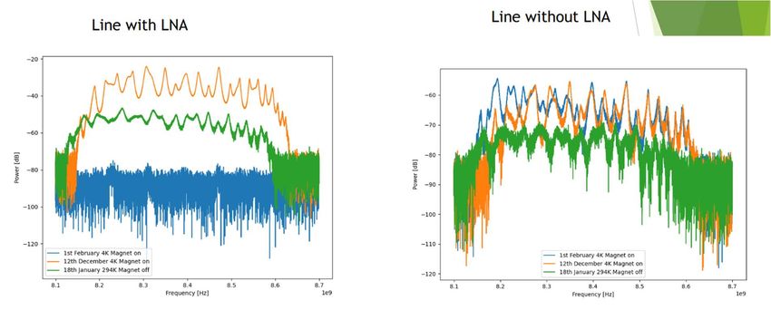
Other sub-projects

3 RADES – High-mass axion search

3.1 Developments since October 2020

3.1.1 Submission of 2018 data-taking results for publication
In the last report we mentioned working on the finalization of the 2018 data-analysis. Between Octo-
ber and April, we worked on several fine details of the analysis such as the impact of the filtering
procedure on a potential axion signal, which we now think has been addressed in a correct fashion.
Consequently, after a collaboration-internal review, the results of the 2018 data-taking campaign of
the CAST-RADES sub detector have been submitted to the arXiv and can be found at
https://arxiv.org/abs/2104.13798 and subsequently to JHEP. For convenience, we show in Figure 3.1
the resulting exclusion limit. The reported results constitute one of the most sensitive high-mass axion
searches, only superseded by a QUAX result recorded at much lower temperatures.

 Figure 3.1: Axion-photon coupling vs axion mass phase-space. In dark red the CAST-RADES
 axion-photon coupling exclusion limit with 95% credibility level presented in this manuscript. The
coupling-mass plane is shown in natural units for consistency with most literature in the field. Inset: Zoom-in
of the parameter range probed in this work (34.6738 µeV

doesn’t originate from the cavity itself. Through a set of measurements we can also almost certainly
exclude a problem with the LNA itself. The most likely explanation for our findings is a problem in
the cryogenic part of the magnet connecting the LNA with the cavity. Since the amplification of the
LNA is needed to observe a potential axion signal, the current status of our set-up is insufficient for
useful physics data. Repair is also impossible without an intervention, which would have stopped the
CAPP data taking for several weeks and thus was not requested.
From the current run we are thus left with 15 useful days of data from 2020 which will be analysed.
Priority until now however was in finishing the 2018 analysis, which has been achieved (see above).

Figure 3.2: Cavity resonances on different dates with (left) and without (right) passing the signal through the
 cryogenic LNA.

3.2 Future possibilities for RADES in CAST
In the event of a continuation of data-taking with CAST, our group’s aim would be to install a setup
promising good physics results avoiding as much as possible the risk of another loss of data. Thus,
even though we have demonstrated the tunability of our cavities in cryogenic environments, we would
be reluctant of a fast installation of a tunable cavity. The reason is that the demonstration of tunability
was performed for manual tuning and a cryogenic motor has not been included in our tests yet.
We have avenues to improve the unloaded quality factor of the currently installed cavity, by removing
and possibly brazing the cavity. The poor unloaded quality factor was at the heart of many issues,
before the cable connection was lost. In case we have on the order of 2-3 months between CAST
reopening and renewed data-taking, such an attempt can well be undertaken and, if successful, could
be expected to yield a good physics result as already proven on 2018 data. In parallel, several R&D
developments for a future data campaign in babyIAXO are ongoing.

4 The new solar axion data taking campaign with the IAXO pathfinder system

 at CAST

4.1 Summary and goals
Solar axion searches were resumed at the sunrise end of CAST detector with the IAXO pathfinder
system, composed by the X-ray optics and an improved, low background and low threshold gaseous
detector. The goal of the current data taking campaign is to:
 1. Improve the result obtained in the 2013-15 phase on .
 20

2. Clarify the statistical/systematic origin of the 2 -excess observed in the sunrise Micromegas
 (SRMM) data set.
 3. Get insight into the limitations of current detection parameters (background and threshold) in
 microbulk technology.
 4. Provide technical and operational experience for the future BabyIAXO and IAXO.

4.2 Preliminary considerations
The last vacuum solar axion data-taking campaign of 2013-15 was a success, providing the best limit
so far on by CAST. The effective background level (number of background counts expected in
the energy- and focal-area-region of interest) is of about 1 count per 6 months of operation of the
experiment (~0.003 counts/hour). However, the relatively low statistics collected with this system in
the 2013-15 campaign (290 tracking hours) makes the result statistics-limited, which partially hinders
its impact in the overall limit.
The current understanding of the background limitations of microbulk detectors allow to devise a
number of steps to carry out in the search for even lower background levels. The opportunity of
operating these improved systems at CAST offers a realistic environment to validate such improve-
ments, specifically the usage of Xe-based gas mixtures.

4.3 Status and achievements
The present data taking has already provided additional statistics at CAST with the mentioned system,
doubling the tracking hours. During the Ar+2.3% isobutane phase (2019-2020) we collected 3030
hours of background, including 152 hours of tracking time, and in the current Xe-based mixture phase
(2020-2021) we have 3425 hours of background including 132 hours of tracking time (as of
17/05/2021). The preliminary analysis shows that the background rate is at the level of ~10-6
c/keV/cm2/s, compatible with the previous result, as it was published in 2017 (Nature Phys. 13 (2017)
584-590).

4.4 Data taking campaign with Xe-based mixtures
We started data taking with a new Xe-based gas mixture, in particular 48.85% Xe + 48.85% Ne +
2.3% Isobutane, in September 2020, after a gas system upgrade to allow for recirculation. The system
works and data have been taken successfully, which is an important technical achievement. The en-
ergy spectrum is free of the 3 keV Ar escape peak and is thus expected to reduce the background in
this energy region. This was an important milestone as the peak of Primakoff produced axion is ex-
pected in that energy.
During data taking in recirculation conditions, we have observed a gain loss with time (Figure 4.1).
After replacing the gas filters and injecting new gas several times, the effect was still present. The
current hypothesis is that permeation of the different gases in the mixture through the window is
different. Isobutane is the biggest molecule among the three, so its relative amount in the mixture
increases. The increase in quencher leads to a lower gain for a given voltage.
The energy threshold is affected by the gain, ranging between 0.8 keV for the higher gain runs and 3
keV for the lower gain runs.
The 25th of March 2021, while a gas injection procedure was being performed, the gas in the bottle
was accidentally lost. We now have a limited amount of gas (~15 l), but the system has been adapted
to the new situation and the response is being satisfactory.

 21

Figure 4.1: Relative gain computed as the 5.9 keV peak position in each of the daily calibration runs. Rele-
 vant interventions or changes in the conditions are annotated.

We found that the conditions and voltages that are required to work with the current Xe-based gas
mixture are pushing the detector to the limit. The current in the mesh shows many spikes, some of
which end up causing trips and occasionally sparks. Some of these sparks have broken channels in
the readout and they had to be disconnected. One of the disconnected channels is close to the centre
of the readout and it will have to be handled carefully during the analysis (Figure 4.2).

 Figure 4.2: Readout channel activity histogram for calibration runs, where signal is focalized in the centre
 of the readout. In red, a run taken before disconnecting one of the central channels and over imposed in
 blue, one of the latest runs. The red channels that can be seen are those that have been lost during the data
 taking period.

4.5 Data analysis
A new public release of the software has been published, including all the developments made during
the last year specifically for CAST: https://github.com/rest-for-physics.

 22

Some of these improvements include new ways of computing the size of the event in the readout XY
plane to better match what we see. The study of the second track has also been implemented, as in
the current setup in which we save all the channels instead of only those that are above a given thresh-
old, we see larger events that many times have more than 1 track. Finally, some noise reduction
strategies are also being tested, which may lead us to reach an even lower energy threshold.
The full datasets, both with Ar and Xe, will be re-analyzed once all the improvements are totally
implemented and well tested.

4.6 Preliminary background spectrum with Xenon
A very preliminary background level including only 1 track events and applying cuts based on 55Fe
calibrations with Xenon has been computed, pointing towards levels of a few 10-6 c/keV/cm2/s. As
seen in Figure 4.3, the argon fluorescence peak at 3 keV no longer appears, reducing the background
level in that range. The somehow larger background above 4 keV is attributed still to imperfections
in the preliminary calibration. The final Xe analysis must wait until the end of the data taking cam-
paign, because we need to calibrate the detector with multiple energies in the X-ray tube lab with the
gas mixture we are currently using.

Figure 4.3: Background spectrum of the SRMM detector during 2015 (black) and 2020/2021 (red). The peak
at ~3keV corresponds to Ar fluorescence and the ~8keV to Cu fluorescence. More than half of the background
counts in the 2–7keV region are in the 3keV peak. Replacing Ar by Xe in the detector (red) makes this peak
disappear and presumably further reduce background. In addition, the contribution from the -decay of the
naturally occurring 39Ar isotope, estimated to about 10-7 counts/keV/s/cm2, would be avoided. The red curve
shows the preliminary background spectrum for 1 track events in runs with xenon, where no peak is seen in
the 3 keV range.

4.7 Low gain runs
During the last days, about 60 hours of low gain background runs have been taken. The aim of these
is to see high energy events such as alphas from Rn, and to quantify their effect especially in the low
energy range of the spectrum. This study is in process and more statistics would be desirable.

 23

5 InGrid/GridPix detector – Search for low energy solar ALPS

The CAST InGrid detector is a gaseous low-background X-ray detector based on a GridPix structure
as gas-amplification device. A GridPix structure consists of a Micromegas-like aluminum grid mount
50 µm above the surface of a charge-collecting pixel CMOS-ASIC, in this case the TimePix ASIC.
A second generation CAST Ingrid detector has been taking solar tracking data in 2017/18 in the focal
plane of the LLNL IAXO-pathfinder X-ray telescope. The detector consisted of seven GridPix struc-
tures. The central GridPix was positioned in the focal spot of the telescope and was surrounded by
six GridPixes acting as veto and augmented with two scintillator based external veto detectors as well
as an FADC readout of the signal induced of the grid. The detector was equipped with an ultra-thin
200nm X-ray entrance window significantly improving efficiency in the

The suspected reason for the time-dependence is a time-dependence of the gas gain, e.g. due to tem-
perature, pressure or other residual gas contamination.
The default energy calibration works as follows in a simplified form:
 (1) Compute the gas gain of each run for both background (typically 2-4 day long) and calibration
 (2h long).
 (2) Fit all 55Fe spectra of the calibration runs, including the escape peak. Photo and escape peaks
 are used for a linear energy calibration (i.e. charge-to-energy conversion factor).
 (3) From all linear fits of the calibration runs, perform a linear fit of all gas gains versus the
 calibration factors of each individual calibration. This yields a function which maps gas gain
 values to energy calibration factors.
Use the computed function of (3) to calculate the energy for each cluster in background and calibra-
tion runs, by using the gas gain value computed for each run as the input.

This calibration procedure ensures to be insensitive to gas gain variations from run to run. If the gas
gain, however, changes within a run, the calibration becomes unreliable as can be seen in Fig. 1 left.
To mitigate the effect, we now determine the gas gain at regular time intervals (here: every 90 min).
This time is long enough to collect sufficient statistics in the “Polya” distribution, i.e. the charge per
pixel distribution. On the other hand, the time is short enough compared to the typical time scale at
which significant gas gain changes occur. The energy calibration then is modified to use the corre-
sponding gas gain values for each cluster as an input to the fit function derived in point 3. As can be
seen in Figure 5.1 (right), this new procedure results in a much flatter median cluster energy over
time. The observed statistical fluctuation of the median cluster energy can be minimized by optimiz-
ing the time bin width where 90 min appear an optimal compromise. Longer time scales would intro-
duce visible time variation. In the course of this study, it was also observed that the occasional occur-
rence of very highly ionizing tracks (e.g. from alpha particles) may lead to a bias is the “Polya”
distribution towards large charge depositions. Single events led to outliers in the energy calibration.
These events, which can be easily identified are now removed from the analysis, which also leads to
a significantly more stable energy calibration run-by-run.
Based on this improved calibration procedures, the analysis will now be repeated step by step with
possible fixes or improvements on the way.

5.2 Optimization of energy-dependent likelihood selection
It was observed since long, that for energies below ~1keV the observed background level (after full
software rejection) is higher than above 1 keV. This can be understood since the number of electrons
is proportional to the energy making it harder to distinguish a low-energy deposition from back-
ground. Previously, the likelihood cut to select candidate events was tuned such that for each energy
bin the efficiency remained constant at 80%. We now studied more systematically if this tuning is
optimal in terms of sensitivity. We varied the likelihood cut bin-by-bin and the expected limit on gae
(for fixed gaγ) in each bin (for the current, preliminary overall settings of the analysis). For most high-
energy bins, there was only a weak dependence on the precise choice of the likelihood cut. However,
variations of the cut in the

background taking advantage of the possibility to implement systematic uncertainties more rigorously
via nuisance parameters. This approach makes it also more easy to make better use of the spatial
distribution of the observed events. The background level increases considerably toward the corners
of the chip. This is currently only reflected by considering a fixed fiducial region (“gold region”) in
the center of the chip. However more position information can be exploited included the expected
signal distribution from solar axions and/or solar chameleons.

5.4 Further improvements
Preliminary studies had shown that the impact of simple veto algorithms from the six surrounding
chips, from the scintillators and from the FADC grid readout is only moderate. However, in particular
for the six outer chips, not all information has been exploited so far. A new attempt will be made to
optimally use this information.

In summary, the analysis of the CAST Ingrid data is progressing slowly but steadily. Surely one,
ideally two more publications with physics results are planned. A technical publication on the second
generation CAST Ingrid detector is also in preparation. Given the recent progress, the finalization of
the analysis by the end of 2021 appears feasible.

6 KWISP – Chameleon Search with an opto-mechanical detector

The KWISP opto-mechanical force sensor, in its latest 3.5 version, is now online at the CAST exper-
iment at CERN after a long delay in activities caused by the persisting health emergency. During this
suspension the efforts were directed to data analysis instead. At present the data taking has been
restarted and we expect to collect about 10 hours of sun-tracking data.

6.1 Introduction
Recall that the chameleon search at CAST uses the existing X-ray telescope to focus the hypothetical
solar chameleon flux on the sensitive element of the KWISP opto-mechanical detector and does not
require a magnetic field. Therefore it is operated in a parasitic fashion with respect to the ongoing
axion searches.
We report here on the status and activities conducted in the last period. In particular the membrane
longitudinal position control was put in place and a completely new chameleon chopper was designed,
built and installed in the system. In parallel the data from the previous measurement campaigns were
fully analyzed.

6.2 KWISP 3.5 set-up
KWISP 3.5 is based on a high finesse Fabry-Perot (FP) resonant cavity with a thin membrane made
of stoichiometric silicon nitride placed in the middle. This setup transduces sub-nm displacements of
the membrane into a cavity detuning which is easily detected in the frequency locking feedback loop.
Here the displacements might have been caused by the radiation pressure of particle beam and can be
translated into a force by an equivalent spring constant of the membrane which is frequency depend-
ent. This mechanical impedance was separately determined in a dedicated setup based on a Michelson
interferometer [1]. A special feature of the KWISP 3.5 setup is a chameleon chopper placed in the
chameleon beam before the detector. The chopper modulates the beam at a predetermined frequency
thus allowing for easy identification of the interaction of the chameleon beam with the sensor in the
detuning spectra of the FP cavity.

 26