Data Assimilation Predictive GAN (DA-PredGAN): applied to determine the spread of COVID-19
←
→
Page content transcription
If your browser does not render page correctly, please read the page content below
Data Assimilation Predictive GAN (DA-PredGAN): applied
                                                    to determine the spread of COVID-19
                                                       Vinicius L S Silva∗,1,2     Claire E Heaney1,2              Yaqi Li2
                                                                           Christopher C Pain1,2,3

                                                                                  June 21, 2021
arXiv:2105.07729v2 [cs.LG] 18 Jun 2021

                                                    1
                                                      Applied Modelling and Computation Group, Imperial College London, UK
                                                   2
                                                    Department of Earth Science and Engineering, Imperial College London, UK
                                               3
                                                 Data Assimilation Laboratory, Data Science Institute, Imperial College London, UK
                                                                 ∗
                                                                   Corresponding author email: viluiz@gmail.com

                                         Abstract
                                         We propose the novel use of a generative adversarial network (GAN) (i) to make predictions
                                         in time (PredGAN) and (ii) to assimilate measurements (DA-PredGAN). In the latter case,
                                         we take advantage of the natural adjoint-like properties of generative models and the ability
                                         to simulate forwards and backwards in time. GANs have received much attention recently,
                                         after achieving excellent results for their generation of realistic-looking images. We wish
                                         to explore how this property translates to new applications in computational modelling
                                         and to exploit the adjoint-like properties for efficient data assimilation. To predict the
                                         spread of COVID-19 in an idealised town, we apply these methods to a compartmental
                                         model in epidemiology that is able to model space and time variations. To do this, the
                                         GAN is set within a reduced-order model (ROM), which uses a low-dimensional space
                                         for the spatial distribution of the simulation states. Then the GAN learns the evolution
                                         of the low-dimensional states over time. The results show that the proposed methods
                                         can accurately predict the evolution of the high-fidelity numerical simulation, and can
                                         efficiently assimilate observed data and determine the corresponding model parameters.

                                         Keywords: generative adversarial networks; spatio-temporal prediction; data assimila-
                                         tion; reduced-order model; deep learning; COVID-19.

                                         1    Introduction
                                         A combination of the availability of large data sets, the advances in algorithms and the
                                         accessibility of computational power has resulted in an unparalleled surge of interest in
                                         machine learning, and subsequently significant advances have been made in many different
                                         fields. Machine learning can be seen as a process of solving practical problems by build-
                                         ing a statistical model based on a given dataset. This building process can be broadly
                                         classified as supervised learning, when there is the presence of the outcome variable to
                                             Source code and data are available at https://github.com/viluiz/gan

                                                                                         1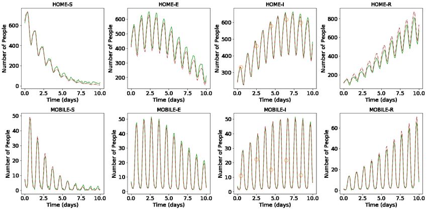
guide the learning process, or unsupervised learning, when there are only the features and
no measurements of the outcome. In the latter, the main goal is to describe how the
data is organised or clustered [1]. Recently, a class of machine learning methods referred
to as deep learning (for either supervised or unsupervised problems) have been achieving
extraordinary results, surpassing the ones obtained from previous machine learning tech-
niques [2–4]. Based on artificial neural networks, deep learning techniques use multiple
layers to extract features or patterns progressively from the data. Examples of this can
be found in pioneering work by LeCun et al. [5], using convolutional neural networks, and
by Rumelhart et al. [6], using recurrent neural networks.
    Deep generative models are one type of unsupervised learning and aim to generate
samples from complex probability distributions in high-dimensional spaces [2]. They learn
the structure of the input data (which has an unknown closed form) and can be used to
generate new instances that appear to have been taken from the training data. There are
several types of generative models including deep belief networks (DBN) [7], variational
autoencoders (VAE) [8], and the generative adversarial network (GAN) [9]. Here, we
focus our attention on the latter. A GAN comprises two networks, a generator and a
discriminator. During training, the former produces samples (so-called “fake samples”)
from a set of random variables, and the second network attempts to distinguish between
samples drawn from the training data and the fake samples. After training, the generator
can be used to produce realistic samples, and the discriminator can be used to distinguish
between samples. Although originally developed within the field of image generation, more
recently, applications of GANs in computational physics have emerged. These applications
attempt to exploit the capabilities of GANs, and predict realistic spatially and temporally
varying solutions. For example, Gupta et al. [10] tackle the problem of predicting human
trajectories using a novel GAN based encoder-decoder framework. Their proposed method
predicted socially plausible futures that outperformed prior works. Xie et al. [11] address
the problem of super-resolution fluid flows by using a GAN to infer three-dimentional
volumetric data in time. They used two discriminators, one that focuses on space while
the other focuses on temporal aspects. Zhong et al. [12] proposed a conditional GAN as
a surrogate model for predicting the migration of carbon dioxide plumes in heterogeneous
reservoirs. Their results show high accuracy prediction in space and time when compared
with a compositional reservoir simulator. Cheng et al. [13] used a GAN to make spatio-
temporal predictions of a nonlinear fluid flow. They demonstrate that the results of the
GAN are comparable with those from the high-fidelity numerical model. All of the previous
works tackled the problem of spatio-temporal model prediction. In addition to predicting
in time, for many practical applications, being able to assimilate observed data is highly
desirable.
    Data assimilation is an inverse problem with the aim of calibrating uncertain model
parameters in order to generate results that match observed data within some tolerance
[14–17]. Some researchers used GANs to tackle this specific problem. Mosser et al. [18]
trained a GAN to represent the prior distribution of subsurface properties and integrated
it within a data assimilation framework based on adjoint capabilities. Kang and Choe
[19] proposed a method where a cluster technique using principal component analysis
(also known as proper orthogonal decomposition) and K-means is performed in the prior
models to select realisation that match the observed data. Then a GAN is trained on
these realisations in order to generate calibrated models. Razak and Jafarpour [20] used
a similar approach of clustering the prior models; however, they also apply a conditional
GAN to label production responses of each model. Canchumuni et al. [21] compared
different deep generative networks formulations, including GANs and VAE, integrated with

                                            2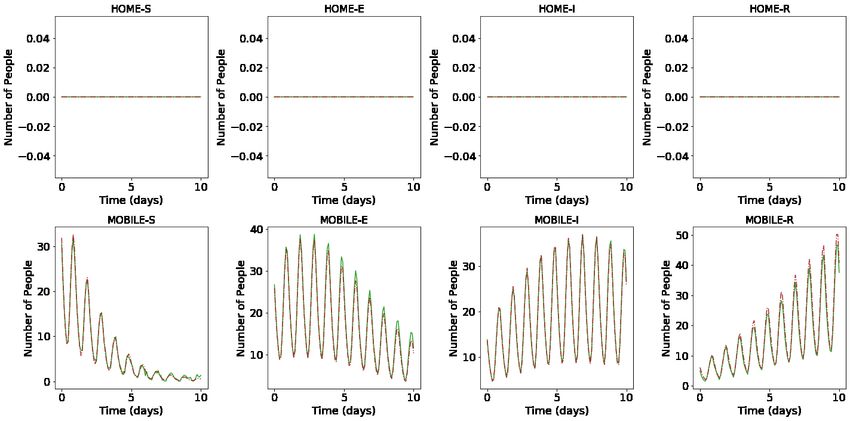
a Kalman filter-based method for proper data assimilation of facies models in reservoir
simulations. A common characteristic of these works is that they use GANs in order to
generate the model parameters. The forward simulations (spatio-temporal predictions)
still need to be performed using the high-fidelity numerical simulator. In this work, we
propose two contributions: the generation of spatio-temporal predictions using GANs and
the assimilation of observed data using GANs. In the first contribution, an algorithm is
developed so that a GAN is able to make predictions in time (PredGAN) for unseen model
parameters. After the GAN has learnt the evolution of the system, an iterative process is
applied to the generator in order to march forward in time. In the second contribution,
the iterative process is extended in order to assimilate observed data and generate the
corresponding model parameters (DA-PredGAN). No additional simulation of the high-
fidelity numerical model is required during the data assimilation process adding to the
efficiency of this method.
     The test case chosen here is the spatio-temporal variation of a virus infection in an
idealised town. Where possible, parameters of the model were chosen to be consistent with
those of COVID-19. With compartments of susceptible (S), exposed (E), infectious (I) and
recovered (R), the extended SEIRS equations [22] are used to generate the high-fidelity
numerical simulations that describe the spread of infections in both space and time. Based
on differential equations, multi-compartment SEIR-type models [23, 24] can be very costly
to solve: there may be millions of variables every time step; and the time steps may need
to be small to model the movement of people around the domain. When applied to a city,
a country or the entire world, solving such models can therefore require substantial com-
putational resources. In order to reduce the computational cost of numerical simulations,
reduced-order models (ROM) are now commonly used for applications in computational
physics [25, 26]. Nonetheless, they are relatively new to virus modelling [22]. A ROM
is a low-dimensional representation of a high-dimensional model or discretised system,
and should be accurate enough for the desired use and at least several orders of magni-
tude faster to solve than the high-dimensional system. Three steps are involved in their
construction: (i) generation of solutions of the high-dimensional system (snapshots), (ii)
compression of the snapshots to find a low-dimensional space for the approximation, and
(iii) approximation of the high-dimensional system in the low-dimensional space. The low-
dimensional space is often found with methods based on singular value decomposition, such
as proper orthogonal decomposition (POD) [27], although autoencoders offer a promising
alternative [28]. In the third step, the high-dimensional system is projected onto the
low-dimensional space for a projection-based ROM [29], whereas for a non-intrusive ROM
(NIROM), the snapshots are projected onto the low-dimensional space and the dynamics
of the system in this space for unseen parameters are represented by interpolation. This
can be performed by classical interpolation methods such as cubic splines [30] or radial
basis functions (RBF) [31]. The RBF approach was extended by [32] who used a Smolyak
grid to sample the parameter space; by [33] who interpolated values of model parameters
and time levels using one parametrisation; and by [34] who used adaptive sampling in
time. Recently, neural networks have been used to perform the interpolation, and exam-
ples of this for steady-state parametrised problems can be found in [35, 36], both of whom
use POD and multi-layer perceptrons, and in [37], who use POD and compare a number
of different networks. Examples for time-dependent parametrised problems can be found
in [38], who used feed-forward neural networks to model the viscous Burgers’ equation;
[39], who proposed a nested trio of networks to learn spatial patterns, temporal patterns
and to learn the dependence on the model parameters; [40], who combine convolutional
autoencoders with recurrent neural networks for Burgers’ equation and the shallow wa-

                                            3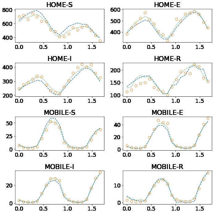
ter equations; [41, 42], both of whom combine an autoencoder and a feed-forward neural
network; and [43], who train an multi-layer perceptron with data from both high-fidelity
and low-fidelity models to improve the accuracy of the model. In this paper, we set the
PredGAN and DA-PredGAN algorithms within a NIROM framework, using POD for the
compression step and a GAN for learning how the dynamics depend on the model parame-
ters. However, both PredGAN and DA-PredGAN could also be used without the NIROM
framework (for smaller problems).
    The main novelties of this research involve the application of a new GAN approach
to both spatio-temporal prediction and data assimilation. This requires an additional
optimisation every time step in order to be able to use the generator within the GAN
for predictions. This optimisation proves to be well suited to data assimilation problems
using adjoints and gradient-based approaches. It is worth mentioning that this method is
not limited to the underlying physics. It is a general framework for developing surrogate
models and assimilating observed data.
    This paper is structured as follows: the next section (Section 2) provides the description
of the proposed method for spatio-temporal prediction and data assimilation with GANs.
Section 3 introduces the test case, a spatio-temporal compartmental model in epidemiology.
After that, the results of the prediction and data assimilation are presented in Section 4.
Section 5 presents some further discussions. Finally, concluding remarks are provided in
Section 6.

2     Method
In this section, firstly a method to make spatio-temporal predictions using a GAN is
proposed. This algorithm is set within a NIROM framework in order to reduce the number
of variables that the GAN has to work on, however, for problems with fewer degrees of
freedom, this may not be necessary. The NIROM involves finding a low-dimensional space
in which to approximate high-dimensional model snapshots of a high-fidelity numerical
simulation. The GAN then learns the evolution of the numerical simulation based on the
evolution of the snapshots in the low-dimensional space. Therefore, the aim of predicting
in time using GANs is to be a surrogate model for the high-fidelity numerical simulation.
Secondly, considering we have observed data, we can extend the forecasting using GANs to
match the given data and generate the model parameters, without running any additional
simulations of the high-fidelity numerical model.

2.1   Predicting in space and time using GANs
Proposed by Goodfellow et al. [9], GANs are unsupervised learning algorithms capable of
learning dense representations of the input data, and can be used as generative models:
they are capable of generating new samples following the same distribution of the training
dataset. The training is based on a game theory scenario in which the generator network G
must compete against an adversary. The generator network directly produces samples from
a random distribution as the input (latent vector z) and its adversary, the discriminator
network D, attempts to distinguish between samples drawn from the training data and
samples drawn from the generator. The output of the discriminator D(x) represents
the probability that a sample came from the data rather than a “fake” sample from the
generator. The output of the generator G(z) is a sample from the distribution learned from
the dataset. Eqs. (1) and (2) show the loss function of the discriminator and generator
used in this work, respectively,

                                              4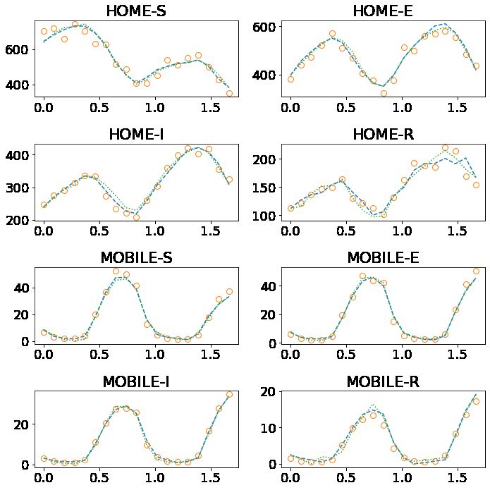
LD = −Ex∼pdata (x) [log(D(x))] − Ez∼pz (z) [log(1 − D(G(z)))] , (1)
LG = Ez∼pz (z) [log(1 − D(G(z)))] . (2)
In order to make predictions in space and time using a GAN, here an algorithm named
Predictive GAN (PredGAN) is proposed. We train a GAN to be able to generate the
following nonlinear map
G(zn ) = Φn , (3)
between the latent variables, zn at time level n, and the solution generated by the GAN
Φn . The Φn is made up of m consecutive time steps of compressed variables α (compressed
spatial outputs of the numerical simulation) which are proper orthogonal decomposition
(POD) coefficients, but could also be latent variables from an autoencoder, and the vector
µ of parameters used within the high-fidelity model (e.g. a material property, or other
simulation input). For a GAN that has been trained with m time levels, Φn takes the
following form
(αn−m+1 )T , (µn−m+1 )T
(αn−m+2 )T , (µn−m+2 )T
.
Φn =
.. ,
(4)
(α n−1 T
) , (µ n−1 )T
n T
(α ) , (µ )n T
where (αn )T = [α1n , α2n , · · · , αN
n
POD
] and (µn )T = [µn1 , µn2 , · · · , µnNµ ]. NPOD is the number
of POD coefficients, αin represents the ith POD coefficient at time level n, Nµ is the number
of model parameters, and µni represents the ith parameter at time level n.
By design, the generator of a GAN produces realistic-looking solutions (images) from
a randomly-generated set of latent variables. In order to predict in time we have to modify
the way in which the GAN is used. When predicting with a GAN trained to produce m
time levels simultaneously, we need to know the first m − 1 time levels in order to predict
a future value, i.e. from known solutions at time levels {0, 1, · · · , m − 2} we can predict
the solution at time level m − 1. To predict the next time level, we use known solutions
at time levels from {1, 2, · · · , m − 2} and the newly predicted solution at time level m − 1,
to predict the solution at time level m.
Assume we have the solutions at time levels up to and including m − 2 for the POD
coefficients, denoted by {α̃k }m−2 k=0 , and consider model parameters known over the entire
simulation time µ̃k , then to predict future solutions:
1. a latent vector (0) zm−1 is randomly generated in order to start the prediction of
time level m − 1. The superscript in brackets on the left of the latent vector is the
optimisation iteration counter within a time step prediction;
2. time iteration counter is set to n = m − 1;
3. optimisation iteration counter is set to l = 0;
4. the generator of the GAN is evaluated at the current value of the latent variables,
(l) zn , yielding
G((l) zn ) = (l) Φn ; (5)
5
5. the difference between the predicted values and the known values is calculated:

                           n−1
                           X                       T
        Lp ((l) zn ) =                 α̃k −(l)αk        Wα α̃k −(l)αk
                         k=n−m+1
                                                         n−1
                                                         X                 T
                                               +               ζµ µ̃k −(l)µk Wµ µ̃k −(l)µk , (6)
                                                    k=n−m+1

      where Wα is a square matrix of size NPOD whose diagonal values are equal to the
      weights that govern the relative importance of the POD coefficients. All other entries
      are zero. The weights could be based on the singular values if a POD method is used
      for compression, for example. Wµ is a square matrix of size Nµ whose diagonal
      values are equal to the model parameter weights, and the scalar ζµ controls how
      much importance is given to the model parameters compared to the compressed
      variables. It is worth mentioning that the goal in each time iteration is to predict a
      new time level n, hence the POD coefficients αn and model parameters µn of this
      time level are not in the loss function.

  6. the gradient of the loss Lp is calculated with respect to the latent variables (l) zn
     (by back-propagation), and Lp is minimised in the gradient direction leading to an
     updated set of latent variables (l+1) zn ;

  7. the optimisation iteration counter is incremented by one (l ← l + 1);

  8. steps 4 to 7 are repeated until convergence is reached;

  9. the converged latent variables are saved as zn (note, no optimisation iteration index)
     and used to initialise the latent variables at the next time level, (0) zn+1 = zn . The
     predicted time step n is added to the known solutions α̃n = αn ;

 10. the time iteration counter is incremented by one (n ← n + 1);

 11. go back to step 3 (until the final time level is reached).

    It is worth mentioning that the gradient of Eq. (6) can be calculated by automatic
differentiation [44–46]. In other words, minimising the loss in Eq. (6) can be achieved
simply by back-propagating the loss through the generator using the same methods that
were employed when training the GAN. Figure 1 illustrates how the PredGAN works for a
generator trained to produce a sequence of 3 time steps (i.e. m = 3). One important aspect
of this predictive GAN approach to time stepping is that it never tries to extrapolate, only
interpolate previous data. Thus the results of this model will always look realistic if the
GAN is well trained and every point in the latent space z produces realistic looking models.

2.2   Data assimilation using GANs
Data assimilation is an inverse problem that aims to combine a mathematical model with
observations [14, 47]. Data assimilation can be executed naturally by GANs due to their in-
herent adjoint-like nature. To perform data assimilation with GANs, we propose a method
named Data Assimilation Predictive GAN (DA-PredGAN) that performs the following
changes in the prediction algorithm (PredGAN). First, one additional term is included in
the functional (loss) in Eq. (6) to account for the data mismatch between the generated
values and observations. Secondly, instead of knowing the model parameters µk , as in the

                                                         6
Figure 1: One time iteration of the PredGAN for a sequence of three time levels (m = 3).
prediction, for the data assimilation the goal is to match the observed data and determine
the values of µk . Thirdly, the forward marching in time is now replaced by forward and
backward marching.
2.2.1 The functional for a time level
Analogous to the definition of Φ in equation (4), the primitive variables vector and obser-
vations vector are defined as
k
(uobs )k1
u1
uk k (uobs )k2
k 2 obs
u = . , u = (7)
. ..
. .
ukNc (uobs )kNc
in which the primitive variable at node j of the spatial grid and time level k is ukj , and
the observation at node j of the spatial grid and time level k is (uobs )kj . Nc is the number
of nodes or cells in the grid. For the forward march, we perform the same process as the
prediction in time (Section 2.1); however, the functional for time level n is now written as
n−1
X T
n
Lda,f (z ) = α̃k − αk Wα α̃k − αk
k=n−m+1
n−1
X T
+ ζµ µ̃k − µk Wµ µ̃k − µk
k=n−m+1
n−1
X T
+ ζobs uk − (uobs )k Wuk uk − (uobs )k , (8)
k=n−m+1
where Wukis a square matrix of size Nc whose diagonal values are equal to the observed
data weights, and the scalar ζobs direct controls how much importance is given to the data
7mismatch. The values in the diagonal of Wuk are set to zero where we have no observation.
The subscript f of Lda indicates that this loss function applies to the forwards march.
In the previous section, before the GAN can start predicting in time, it requires m −
1 known solutions of the POD coefficients {α̃k }m−2 k=0 corresponding to the first m − 1
k
time levels, and the model parameters µ̃ over all simulation time. There are two sets
of POD and model variables: a set of known variables (α̃k , µ̃k ) and a set of predicted
values (αk , µk ). When assimilating data, we usually do not know the values of the model
parameters, hence the aim is to match the observed data and determine the corresponding
µk . To this end, during a time iteration of the forward and backward marches the known
variables of the model parameters are updated by the newly predicted time step µ̃n = µn ,
the same way as for the POD coefficients (item 9 of the prediction process, Section 2.1).
This gives the best approximation to these variables and allows them to vary during the
data assimilation process. Furthermore, after the forward march the solutions at the last
m − 1 time levels are used as known solutions to start the backward march, and after a
backward march the solutions at the first m − 1 time levels are used as known solutions
to start the next forward march.
For marching backwards in time, the loss function should be modified thus
n+m−1
X T
n
Lda,b (z ) = α̃k − αk Wα α̃k − αk
k=n+1
n+m−1
X T
+ ζµ µ̃k − µk Wµ µ̃k − µk
k=n+1
n+m−1
X T
+ ζobs uk − (uobs )k Wuk uk − (uobs )k , (9)
k=n+1
where the subscript b of Lda indicates that this loss function applies to the backwards
march. It is worth noting that the only difference between Eq. (8) and Eq. (9) is the
indices in the summation. For the backward march, given the solution at time levels
{n + m − 1, n + m − 2, · · · , n + 1}, we can predict the solution at time level n. Then, to
predict the next time level we use known solutions at time levels from {n + m − 2, n + m −
3, · · · , n + 1} and the newly predicted solution at time level n, to predict the solution at
time level n − 1. We continue the process until predicting the first time step. After the
backward march, we calculate the average data mismatch, between the predicted primitive
variables and the observed data (last term on the right of Eqs. (8) and (9)), through all
the last backward and forward iterations. The process continues with a new forward and
backward march until the average mismatch has converged or the maximum number of
forward-backward iterations is reached.
2.2.2 Observations of the primitive variables
If proper orthogonal decomposition is used to compress the grid variables, in which
uk = Bαk + u, (10)
a functional contribution that can be used directly within the optimiser is
X T
Lobs (zn ) = ζobs Bαk + u − (uobs )k Wuk Bαk + u − (uobs )k , (11)
k
8where the columns of the matrix B are the basis functions which relate the high-dimensional
solution variables to the POD coefficients, and u is the mean of the ensemble of snapshots
for the variable u.
Having written the solution in terms of the compressed variables when calculating
the mismatch of the observations, the final version of the functional for the forward and
backward march is
X T X T
Lda (zn ) = α̃k − αk Wα α̃k − αk + ζµ µ̃k − µk Wµ µ̃k − µk
k k
X T
+ ζobs Bαk + u − (uobs )k Wuk Bαk + u − (uobs )k , (12)
k
where for the forward march k ∈ {n−m+1, n−m+2, · · · , n−1} and for the backward
march k ∈ {n + m − 1, n + m − 2, · · · , n + 1}.
2.2.3 Applying relaxation
To stabilise the process of marching forwards and backwards, a relaxation parameter is used
in the resulting latent vector zn at each time iteration. After performing an optimisation
using Eqs. (8) or (9), the resulting latent vector is relaxed by
zn = (1 − rj )zn−1 + rj ẑn (13)
where ẑn is the resulting latent vector generated in each time iteration by minimising
Eqs. (8) or (9). j represents a iteration corresponding to a entire forward and backward
march, and rj is the relaxation factor used in the iteration j. Thus each relaxation
parameter rj is used in all time iterations n within the forwards and backwards march.
The relaxation factor rj starts the data assimilation process with the value one. If the
average data mismatch at j is greater than at j − 1, then rj = rj /2 and the forward and
backward iteration j is repeated. On the other hand, if the average data mismatch at j is
less than at j − 1, the algorithm goes to the next iteration j + 1 using rj+1 = 1.5rj , also
respecting the maximum value of one for the relaxation factor (if rj+1 > 1 then rj+1 = 1).
2.2.4 Data assimilation algorithm through time
To assimilate data through time the following steps are performed:
1. march forward in time using the Eq. (6) and the prediction process in Section 2.1,
with guessed parameters {α̃k }m−2 k
k=0 for the first m − 1 time steps and µ̃ over all
simulation time. This will results in an initial guess of αn at all time levels n.
2. Time march backwards in time optimising Eq. (9), starting from the m − 1 final time
levels (obtained from the previous iteration). This tries to perform time stepping
while attempting to match the observations using the observed data mismatch part
of the functional (last term on the right of Eq. (9)). During the time march update
the model parameters using the newly predicted time step µ̃n = µn .
3. Keep time stepping forwards till the end of time and then backwards to the start
of time using Eqs. (8), (9) and (13), until the algorithm has converged. We use as
convergence criteria rj < 0.01.
94. If there are parameters αn and µn changing rapidly during the data assimilation
process increase the corresponding weight (in Eqs. (8) and (9)) and if they are not
changing rapidly enough decrease it.
5. After convergence, perform a last forward march using the Eq. (6) and the prediction
process in Section 2.1. Use the last calculated parameters {α̃k }m−2 k
k=0 and µ̃ for this.
Figure 2 shows an overview of the DA-PredGAN algorithm.
Figure 2: Overview of the DA-PredGAN process.
2.3 Weighting terms in the functionals
We suggest giving the data mismatch part of the functional greater priority than the time
stepping part of the functional. Considering that we set non-zero terms on the diagonal
of Wuk to one, then
!
∆α 2 (m − 1) N
P POD
(w α )ii
ζobs = ζ̂obs P PNi=1 , (14)
∆u k
c k
i=1 (wu )ii
where ζ̂obs is a tuning parameter and in this work it is set to 10. ∆α and ∆u are the
ranges of the compressed variables and the primary variables, respectively. (wα )ii are the
the terms on the diagonal of Wα , and (wu )kii are the terms on the diagonal of Wuk . For
the forward march k ∈ {n − m + 1, n − m + 2, · · · , n − 1} and for the backward march
k ∈ {n + m − 1, n + m − 2, · · · , n + 1}.
ζµ controls how quickly one lets the parameters µ change within the data assimilation
method. We choose to set all the terms on the diagonal of Wµ to one, and
!
∆α 2
PNPOD
i=1 (wα )ii
ζµ = ζ̂µ PNµ , (15)
∆µ (wµ )ii
i=1
10where ∆µ represents the range of the scalar parameters, (wµ )ii are the the terms on the
diagonal of Wµ , and ζ̂µ is a tuning parameter. In this work, we use ζ̂µ = 10−2 for the
prediction, and the first and last forward marches of the data assimilation. For the other
forward and backward marches of the data assimilation we can choose to dynamically
update ζµ , in order to let µk change more rapidly at the beginning and more slowly when
the process is near convergence. Therefore, we start with ζ̂µ = 10−4 and increase it by a
factor of 1.2 after each forward-backward iteration.
3 Test case
3.1 Compartmental models in epidemiology
The current COVID-19 pandemic, caused by the virus SARS-CoV-2, is something without
precedent in modern history, although it follows the same rules common to other pathogens
[48]. The knowledge gathered during more than one century studying these outbreaks has
given rise to a well-founded theory of the dynamics of infectious diseases [49, 50]. One
of the simplest nonlinear models to describe the spread of an infection is the SIR model,
which consists of a system of ordinary differential equations where S, I and R represent
the number of people who are susceptible, infectious or recovered [49, 51] referred to as
compartments.
The model starts by considering a population of N individuals in the susceptible com-
partment. If one individual with the disease is introduced into the population, over time,
other people will become infected and move into the infectious compartment. The mem-
bers of the infectious compartment will spread the pathogen among the population until
they recover. This is called a “closed epidemic” for which N = S + I + R. The SIR model
assumes that the population mixes at random and that it is large enough for averages to
be used meaningfully [50, 51]. One important factor in the dynamics of infectious diseases,
and consequently in the SIR model, is the basic reproduction number (R0 ) [52]. It rep-
resents the expected number of secondary cases caused by a single infected member in a
completely susceptible population. Knowing the magnitude of the R0 gives an indication
of how rapidly the infection could spread, allowing governments and authorities to esti-
mate the amount of effort necessary to prevent, diminish or eliminate an infection from a
population [53]. Following this line, much effort has been committed to estimating the R0
in the COVID-19 pandemic worldwide [54–57].
Albeit simple, the SIR model can provide important insights into the dynamics of
infectious diseases in an idealised population. Nonetheless, for more realistic situations
other factors need to be taken into account such as births, deaths and loss of immunity.
Furthermore, it is well known for most diseases that there is an incubation period between
being infected and becoming infectious [58]. For that reason the SIR model can be extended
to the SEIRS model. In the latter formulation, after being infected an individual is moved
to the exposed compartment (E) and remains there until they become infectious. Also,
recovered people may become susceptible again due to the loss of immunity. Another
important factor regarding the flow in and out of a compartment is demography. Births
and deaths can also be taken into account by adding their rates to the formulations [58].
Other types of compartments can also be added depending on the flow patterns between
the compartments [52, 59].
When large-scale simulations are considered, for example a simulation of spatial-
variation of the COVID-19 infection in a whole city or a country, the computational
time becomes a concern. Additionally, if observed data needs to be taken into account the
11whole process can become impracticable. In order to tackle this problem, we propose a
surrogate model that can be used to replace the forward numerical simulation and it can
also assimilate data without any additional run of the high-fidelity model.
3.1.1 SEIRS model
The classic SEIRS (Susceptible - Exposed - Infectious - Recovered - Susceptible) model
can be represented by the diagram in Figure 3. The diagram shows how individuals move
from one compartment to another.
Figure 3: Diagram of the SEIRS model. It represents the number of people in each compartment
(susceptible, exposed, infectious, recovered) and how they move between them.
In the diagram, S, E, I and R are the number of individuals in the susceptible, exposed,
infectious and recovered compartments, respectively. N represents the total population
size, β is the transmission rate (the average rate at which an infectious individual can
infect a susceptible), σ is the rate of exposed individuals becoming infectious (1/σ is the
average period in the exposed group), γ is the recovered rate (1/γ is the average infectious
period), and ξ is the rate recovered individuals return to the susceptible group (1/ξ is the
average period before loss of immunity). The vital dynamics are represented by η and ν,
where η is the birth rate and ν is the death rate.
The system of differential equations describing the SEIRS model dynamics can be
expressed as
dS βSI
= ηN − + ξR − νS, (16a)
dt N
dE βSI
= − σE − νE, (16b)
dt N
dI
= σE − γI − νI, (16c)
dt
dR
= γI − ξR − νR, (16d)
dt
where each equation represents the dynamics within a compartment [58]. At time t, the
total number of people can be expressed as N (t) = S(t) + E(t) + I(t) + R(t). If the
birth rate is equal to the death rate (η = ν) the total size of the population (N ) remains
constant over time. For this case the associated basic reproduction number is defined as
σ β
R0 = . (17)
(σ + ν) (γ + ν)
For most acute infections, the death rate ν is much smaller than the epidemic rates, thus
in realistic situations it barely affects the evolution of the disease [58].
12Eqs. (16) can be also expanded into the extended SEIRS compartmental equations to
take into account the spatial variation of the disease [22].
3.1.2 Extended SEIRS model
People movement is of paramount importance to model the spread of infection diseases
such as COVID-19. Therefore, this project extends Eqs. (16) in two ways:
1. It includes two people groups, people at home (h = 1) and people who are mobile
(h = 2);
2. It applies transport via diffusion to model the movement of people through the
domain.
As a result, the extended equations could model the daily cycle of night and day for
the transient calculations, in which there is a “pressure” for mobile people to return to
their homes at night and join the home group, and a similar pressure for people to leave
their homes during the day, who will therefore join the mobile group. To accomplish this,
the extended SEIRS model introduces a diffusion term (last term on the right of Eqs. (18))
and an interaction term (penultimate term on the right of Eqs. (18)) to model this process:
P H
∂Sh Sh h0 (βh h0 Ih0 )
X
= ηh Nh − + ξh Rh − νhS Sh − λSh h0 Sh0 + ∇ · (khS ∇Sh ), (18a)
∂t Nh
h0 =1
P H
∂Eh Sh h0 (βh h0 Ih0 )
X
= − σh Eh − νhE Eh − λE E
h h0 Eh0 + ∇ · (kh ∇Eh ), (18b)
∂t Nh
h0 =1
H
∂Ih X
= σh Eh − γh Ih − νhI Ih − λIh h0 Ih0 + ∇ · (khI ∇Ih ), (18c)
∂t 0 h =1
H
∂Rh X
= γh Ih − ξh Rh − νhR Rh − λR R
h h0 Rh0 + ∇ · (kh ∇Rh ), (18d)
∂t 0 h =1
in which H represents the number of people and/or places groups e.g. people at home,
mobile people, people at work in the office, shops, people in hospital. Here, we have two
groups of people, hence H = 2, one representing people at home, h = 1, and the second
representing people that are mobile and outside their homes therefore, h = 2. The diffusion
coefficient is represented by kh and describes the movement of people around the domain.
It is defined for each compartment denoted by a superscript {S, E, I, R}. In addition,
βh h0 determines not only the transmission rate between compartments, but also how the
disease is transmitted from people in group h0 to people in group h. The interaction terms,
λh h0 , control how people move between groups, for example, how people that are in the
mobile group goes to the home group. When moving between groups people remain in the
same compartment, and when moving between compartments, people remain in the same
group.
If we again consider the same value
P for the birth and the death rate in all groups, the
total size of the population (N = h Nh ) remains constant over time. For this case the
associated basic reproduction number for each group is defined as
σh βh h
R0 h = , (19)
(σh + νh ) (γh + νh )
13where we assume βh h0 = 0 when h 6= h0 because the people occupying these groups never
meet i.e. people in their homes never meet mobile people (who are outside their homes).
It is worth mentioning that instead of having the number of people in each compartment
(S, E, I and R) changing only in time, as in Eqs. (16), in the extended SEIRS model,
Eqs. (18), they can vary in space and time. Figure 4 shows, for one position in space (or one
cell in the grid), how people move between groups (home, and mobile) and compartments.
Futher details about the extended SEIRS model can be found in Quilodrán-Casas et al.
[22].
Figure 4: Diagram of the extended SEIRS model for one point in space (or one cell in the grid).
The diagram shows how people move between groups and compartments within the same cell in
the grid. The vital dynamics and the transport via diffusion is not displayed here.
3.1.3 Discretisation and solution methods used
The spatial variation is discretised on a regular grid of NX × NY × NZ control volume
cells. Here we work on a 2D problem, so NZ = 1. We use a five-point stencil and second
order differencing of the diffusion operator, as well as backward Euler time stepping. We
iterate within a time step, using Picard iteration, until convergence of all non-linear terms
and evaluate these non-linear terms at the future time level. To solve the linear system of
equations we simply use forward backward Gauss-Seidel (FBGS) within each group (each
of the variables S1 , E1 , I1 , R1 , S2 , E2 , I2 , R2 ) until convergence and Block FBGS between
groups to obtain overall convergence of the system. This solver is sufficient to solve the
test problems presented here.
3.2 Problem set up of an idealised town
The test case occupies an area of 100km by 100km as shown in Figure 5. We divided this
area in 25 regions, where those labelled as 1 are regions to which people do not travel,
the region labelled as 2 is where homes are located, and regions from 2 to 10 are where
people in the mobile group can travel. Thus people in the home group stay in the region
2. The aim is that most people move from home to mobile group in the morning, travel
to locations in regions 2 to 10, and return to the home group later on in the day. The
extended SEIRS model is used here to model this movement of people around the the
cross-shaped domain in Figure 5, in addition to calculating which compartment and group
14each person is in at a given time t. A person at any time and position within the domain
belongs to one of the two groups, home or mobile, and is in one of the four compartments,
Susceptible, Exposed, Infectious, or Recovered.
1 1 6 1 1
1 1 10 1 1
3 8 4 9 5
1 1 7 1 1
1 1 2 1 1
Figure 5: Domain of the 100km × 100km idealised town showing the different regions. Regions
where people can travel are shown in grey.
Table 1 shows the epidemiological parameters used in this test case. These values
are chosen as they are representative of the COVID-19 infection. Tday is the number of
seconds in one day, and the transmission rates βh h are calculated based on the vales of
the R0 h . To generate the ensemble of simulations for the training and test data, the basic
reproduction number for each group of people is sampled from a uniform distribution
with interval (0, 20). The R0 is the main parameter to control the evolution of infectious
diseases, hence we choose to vary it in the ensemble. We also choose to use a wider range
of variation for the R0 h , in accordance with Kochańczyk et al. [60], than the most common
values estimated for the COVID-19 pandemic. The diffusion coefficients (k) used to model
the spatial movement of people and the interaction terms (λ) are the same as those in
Quilodrán-Casas et al. [22].
Table 1: Parameters for the extended SEIRS model. Tday is the number of seconds in one day.
Parameter Home group Mobile group
Birth and death rate (η = ν) (60 × 365 × Tday )−1
Loss of immunity rate (ξ) (365 × Tday )−1
Exposed to infectious rate (σ) (4.5 × Tday )−1
Recovery rate (γ) (7 × Tday )−1
Reproduction number R0 1 ∼ U (0, 20) R0 2 ∼ U (0, 20)
The simulations are run for 45.5 days with a time step of ∆t = 4000 seconds. We use
uniformly space 10 × 10 control volumes to discretise the domain in Figure 5. Therefore,
each region in Figure 5 comprises four control volumes. We start the simulation with 2000
people in each control volume of region 2 and belonging to the home group. All other fields
are set to zero. The initial condition is that 0.1% of people at home have been exposed to
the virus and will thus develop an infection.
4 Results
In order to generate data with which to train the GAN, we performed 40 high-fidelity
numerical simulations. Each simulation has two different values of R0 h , one for people
15at home and another for mobile people. In the numerical simulation the whole region
in Figure 5 is divided in a regular grid of 10 × 10, totalling 100 cells. Although regions
labelled 1 need not be modelled, solving the system on the whole domain is very efficient
as a structured, regular grid can be used. Considering that each group (people at home
and mobile) has four compartments in the extended SEIRS model (Susceptible, Exposed,
Infectious and Recovered), there will be eight variables for each cell in the grid per time
step, which gives a total number of 8 × 100 = 800 variables per time step. We perform
proper orthogonal decomposition in the 800 variables, in order to work with a low di-
mensional space in the GAN. Figure 6 shows the decay of the singular values. The 15
largest singular values capture > 99.9999% of the variance held in the snapshots. This
was deemed sufficient, so 15 POD coefficients were retained for the NIROM. Hence the
GAN is trained to generate the 15 POD coefficients (αn ) and the two R0 h (µn ), over a
sequence of 10 time levels with a step size of two. This time length is chosen because it
roughly represents a cycle (one day) in the results.
106 15 principal components
300000
103
250000
Singular values
Singular values
100
200000
150000 10−3
100000 15 principal components 10−6
50000 10−9
0
100 101 102 103 100 101 102 103
Dimensions Dimensions
(a) (b)
Figure 6: Proper orthogonal decomposition applied to reduce the dimension of a time snapshot
of the extended SEIRS model from 800 to 15 variables. The plot shows the decay of the singular
values. (a) shows the singular values in a linear scale. (b) shows the singular values in a logarithm
scale.
The GAN architecture is based on that of the DCGAN by [61] and is implemented
using Tensorflow [62]. Figure 7 shows the architecture of the generator and discriminator
used in this work. The generator and discriminator are trained over 5, 000 epochs, and
the size of the latent vector z is set to 100. The 10 time levels are given to the networks
as a two-dimensional array with 10 rows and 17 columns. Each row represents a time
level and each column comprises the 15 POD coefficients and the two values of R0 h . We
choose this configuration, instead of a linear representation, to take advantage of the time
dependence in the two-dimensional array (“the image”). The main goal of this work is to
reproduce the outputs of the high-fidelity numerical model and assimilate observed data
using a GAN.
4.1 Predicting in space and time using the PredGAN
In this section, we use the PredGAN (introduced in Section 2.1) to make predictions of the
spatial and temporal variation of the COVID-19 infection in the idealised town. All the
test cases here are new or ‘unseen’ simulations, generated from values of R0 h that were
not used to train the GAN. The prediction using the PredGAN is performed by starting
with nine time levels from the high-fidelity numerical simulation (known initial solutions)
16Figure 7: Generator and discriminator architectures.
and using the generator to predict the tenth. In the next time iteration we use eight time
levels from the numerical simulation and the last prediction to predict a new point. Then
we repeat this process until the last time step. It is worth mentioning that after nine
time iterations, the PredGAN works only with data from the predictions. Data from the
high-fidelity numerical simulation is used only for the first nine time levels as an initial
condition.
The first result we present here is the prediction of one time level for the values R0 1 =
7.7 and R0 2 = 17.4. The first nine time levels (initial condition) were taken from the high-
fidelity numerical simulation after 21 days from the start of the infection. Figure 8 shows
the spatial variation of the number of people in each group and compartment throughout
the domain. Figure 8a shows the prediction of the PredGAN, Figure 8b shows the actual
result from the numerical simulation, and Figure 8c the absolute difference between them.
All the quantities represent the number of people in a cell of the domain. The mean
absolute error between the ground truth and the prediction is 0.19 and the relative mean
absolute error is 8.9 × 10⁻³ . These results show that the PredGAN was able to predict
accurately the evolution of the extended SEIRS model in space and time, at least for one
time iteration.
Figure 9 shows the same set of results as in Figure 8, except now, we focus on the
prediction at one point in space or one cell in the domain (bottom-left corner of region
2 in Figure 5). Each plot corresponds to the variation of the number of people in each
group and compartment over time. The first nine time levels are used in the optimisation
process of the PredGAN and the tenth time level is actually the prediction of the unknown
solution. When using PredGAN, solutions for the POD coefficients at all 10 time levels
are obtained, and all 10 time levels are shown here for illustration. As explained in
17Section 2.1, PredGAN minimises the difference between the nine known values and its
predictions at these time levels. Once converged, PredGAN’s prediction for the tenth
time level is accepted. There will be small differences between the known values and
predicted values for the first nine time levels, which are shown in Figure 9, but these are
ignored in future calculations as only the tenth time level is added to the known solutions.
Comparable results regarding the error in the prediction were seen at other points in the
domain, therefore we do not present them here. It can be noticed from Figures 8 and
9 that the PredGAN can reasonably predict the outcomes of the high-fidelity numerical
model for simulations that are not in training set of the GAN.
For predicting further in time, we again start with nine time levels from the high-
fidelity numerical simulation and we use the generator to predict the tenth. The next
iterations we use the last predictions as known values and we repeat this process until
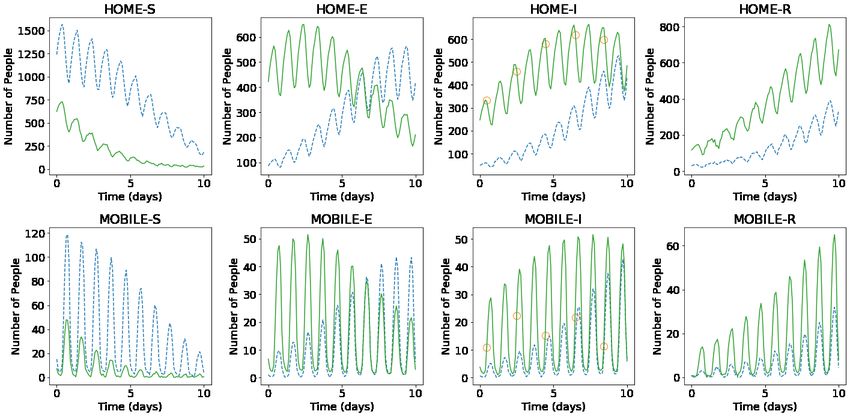
the end of the simulation. Figure 10 shows the result of the prediction in one cell of the
grid (bottom-left corner of region 2 in Figure 5). Each cycle corresponds to a period of
one day, when mobile people leave their homes during the day and return at night. After
the first nine time iterations the PredGAN does not see any data from the high-fidelity
numerical simulation, and relies completely on the predictions from PredGAN. Data from
the high-fidelity numerical simulation is only required as an initial condition. Figure 11
also shows the prediction of the PredGAN, although this time using two more different
sets of values for R0 h and starting at different times of the epidemic dynamics. The results
presented in Figures 10 and 11 indicate that the prediction of multiple time levels was very
successful. For all compartments and groups, the prediction using the PredGAN is almost
indistinguishable from the ground truth or high-fidelity numerical simulation. Hence the
PredGAN can be used as a surrogate model of high-fidelity numerical simulations varying
in space and time.
4.2 Data Assimilation using the DA-PredGAN
In this section, we apply the DA-PredGAN (introduced in Section 2.2) to assimilate ob-
served data to the spatial variation of COVID-19 over time. The data assimilation using
the DA-PredGAN works similarly to the PredGAN, apart from adding an observed data
mismatch term in the functional (Eqs. (8) and (9)), not knowing the model parameters
R0,h a priori, and from working forwards and backwards in time. We generate observed
data from a high-fidelity numerical simulation that was not included in the training set
of the GAN. To that end, we use R0 1 = 7.7, R0 2 = 17.4, and also add 5% noise to
the chosen data. Considering the domain in Figure 5, we choose to have observed data
collected at the bottom-left corner of regions 2, 3, 4, 5 and 6. In other words, the ob-
served data is available at five points in domain, one in the middle and one at each end
of the cross shaped region. The R0 h are not used as observed data, although we compare
it with the true values used to generate the high-fidelity numerical simulation. To start
the DA-PredGAN, we perform one forward march without the observed data term in the
functional (as described in Section 2.2.4). The starting points chosen for this march are
from a numerical simulation with R0 1 = 6.5 and R0 2 = 5.7.
Figure 12 shows the evolution of the forward-backward iterations of the data assimila-
tion process using the DA-PredGAN. The results show the time variation of groups and
compartments in one cell of the grid (bottom-left corner of regions 2). It can be seen from
this figure that in just a few forward-backward iterations the DA-PredGAN is able to
match the data. Although we run the simulation until the convergent criteria was reached
(see Figure 13a), after iteration 2, only small improvements in the observed data mismatch
18can be noticed. This is also shown in Figure 13b, along with the average total loss and the
other average loss terms in the functional (Eqs. (8) and (9)). The evolution of the R0 h for
the same data assimilation is presented in Figure 14. The result shows that as long as the
data mismatch is minimised, the model parameters R0 h approach the true values used to
generate the synthetic observed data. We also present in Figures 15 and 16 a comparison
between the first and the last forward iterations. These figures show that even with the
initial guess far from the observed data the method was able to match the measurements
and produce model parameters R0 h near the true value.
In order to test the DA-PredGAN in a more realistic case, we consider that observed
data is only available every two days, and we measure only infectious people. Figures
17 and 18 show the first and last forward marches of the data assimilation process. We
observe that the method proposed here was able to effectively match the observed data
and to produce model parameters R0 h with similar values as the ones used to generate
the synthetic data. It is worth noticing that the data assimilation is an inverse and
usually ill-posed problem, thus other values of R0 h could have also matched the observed
data, within some tolerance. Figure 19 shows the relaxation factor and the loss terms of
the DA-PredGAN over the forward-backward iterations. These results demonstrate the
efficiency of the DA-PredGAN, since it was capable of matching the observed data in only
few iterations even starting far from the measurements. We also present in Figure 20 a
comparison between the DA-PredGAN results and the high-fidelity numerical simulation
used to generate the observed data. Figure 20a shows the evolution of the number of people
in each group and compartment for a point in space where observed data was collected.
Figure 20b shows the same plots, but for a point in space without observed data. Although
we would not expect that the results of the data assimilation will reproduce the “true”
simulation, since it is a ill-posed inverse problem, we observe from these figures that the
DA-PredGAN was able to generate coherent results that resemble the dynamics of the
ground truth, even at points where observed data was not collected.
5 Discussion
Despite one of the original purposes of generative adversarial networks (GANs), to be able
to generate realistic-looking images, this paper demonstrates that GANs can also be used
to perform spatio-temporal prediction (PredGAN algorithm) and data assimilation (DA-
PredGAN algorithm). The GAN was chosen here because incredible results have been
achieved with this network, clearly outperforming other methods in many applications.
However, other generative models could also fit into the PredGAN and DA-PredGAN
algorithms. We also remark that, although here the proposed methods are set within a
non-intrusive reduced-order model (NIROM) framework, these algorithms could be based
directly on the high-dimensional system. The NIROM was used to reduce the number of
degrees of freedom which makes training the GANs more manageable.
Focusing on the DA-PredGAN, it has the following advantages and disadvantages rel-
ative to other data assimilation algorithms. The advantages are that the DA-PredGAN
has potentially more rapid convergence properties, as even within a few forward-backward
iterations the method was able to match the observed data and update the model pa-
rameters. Furthermore, no additional simulation of the high-fidelity numerical model is
needed to assimilate data using the DA-PredGAN. Another advantage is the use of the
inherent adjoint capabilities of neural networks to calculate the gradients. The error in the
loss functions is back-propagated through the network using the available machine learn-
ing codes e.g. Tensorflow, PyTorch. The primary disadvantage is the need to tuning the
19weighting terms ζobs and ζµ in the loss functions. If not adjusted the method may change
the solution variables prematurely within a forward-backward iteration, or conversely, just
make very small changes to them. To tackle this problem, we have proposed some values
for the weighting terms in Section 2.3. These values have worked well for all the cases we
have run.
6 Conclusion
In this work, we proposed a generative adversarial network that is able to make predictions
in space and time (PredGAN), and we set this within a reduced-order model framework for
efficiency. The aim of the PredGAN is to be a surrogate model of the high-fidelity numerical
simulation. Furthermore, we extended the forecast using generative adversarial networks
to assimilate observed data (DA-PredGAN) without any additional simulations of the high-
fidelity numerical model. We applied these approaches to an extended SEIRS model to
predict the spread of COVID-19 over space and time. The results show that the surrogate
model is able to accurately reproduce the numerical simulation for different model inputs.
We also demonstrate the efficiency of the DA-PredGAN in assimilating observed data
and determining the corresponding model parameters. The proposed methods may have
important implications for a huge class of physical simulation problems, for developing
accurate surrogate models and efficiently assimilating measurements.
20You can also read