Data-Driven Approach for Passenger Mobility Pattern Recognition Using Spatiotemporal Embedding

Hindawi
Journal of Advanced Transportation
Volume 2021, Article ID 5574093, 21 pages
https://doi.org/10.1155/2021/5574093

Research Article
Data-Driven Approach for Passenger Mobility Pattern
Recognition Using Spatiotemporal Embedding

 Chao Yu ,1,2 Haiying Li,1 Xinyue Xu ,1 Jun Liu ,1 Jianrui Miao ,1 Yitang Wang,3
 and Qi Sun4
 1
 State Key Laboratory of Rail Traffic Control & Safety, Beijing Jiaotong University, Beijing 100044, China
 2
 School of Traffic and Transportation, Beijing Jiaotong University, Beijing 100044, China
 3
 Track and Transportation Department, China Railway First Survey and Design Institute, Xi’an, Shaanxi 710043, China
 4
 ACC Technical Room, Beijing Metro Network Control Center, Beijing 100101, China

 Correspondence should be addressed to Xinyue Xu; xxy@bjtu.edu.cn

 Received 8 January 2021; Revised 11 April 2021; Accepted 8 May 2021; Published 19 May 2021

 Academic Editor: Chung-Cheng Lu

 Copyright © 2021 Chao Yu et al. This is an open access article distributed under the Creative Commons Attribution License, which
 permits unrestricted use, distribution, and reproduction in any medium, provided the original work is properly cited.

 Urban mobility pattern recognition has great potential in revealing human travel mechanism, discovering passenger travel
 purpose, and predicting and managing traffic demand. This paper aims to propose a data-driven method to identify metro
 passenger mobility patterns based on Automatic Fare Collection (AFC) data and geo-based data. First, Point of Information (POI)
 data within 500 meters of the metro stations are captured to characterize the spatial attributes of the stations. Especially, a fusion
 method of multisource geo-based data is proposed to convert raw POI data into weighted POI data considering service ca-
 pabilities. Second, an unsupervised learning framework based on stacked auto-encoder (SAE) is designed to embed the spa-
 tiotemporal information of trips into low-dimensional dense trip vectors. In detail, the embedded spatiotemporal information
 includes spatial features (POI categories around the origin station and that around the destination station) and temporal features
 (start time, day of the week, and travel time). Third, a density-based clustering algorithm is introduced to identify passenger
 mobility patterns based on the embedded dense trip vectors. Finally, a case of Beijing metro network is used to verify the feasibility
 of the above methodology. The results show that the proposed method performs well in recognizing mobility patterns and
 outperforms the existing methods.

1. Introduction Fortunately, the continuous development of digitaliza-
 tion has provided strong support for urban planning and
The number of urban residents is increasing significantly, transportation services. Currently, large-scale spatiotem-
and human mobility is becoming unpredictable and com- poral travel-related data provide the possibility for the
plex, posing major challenges to public safety and health analysis of passenger mobility patterns. From the perspective
(such as the COVID-19 epidemic). In recent years, urban of the types of raw data, the recognition of urban mobility
mobility pattern recognition has become a hotspot due to its patterns can be divided into two categories, namely, re-
ability to reveal resident life routines, assist in transportation searches based on trajectory data and that based on AFC
planning, estimate and manage travel demand, predict data. The former is mainly meant to reproduce the move-
passenger travel purposes, and provide location-based ser- ment track of residents through GPS data, social media data,
vices [1–5]. As an important part of urban transportation, or mobile phone signaling data to identify mobility patterns
the metro system has increasingly become an indispensable [6–12]. Unlike this, the latter often uses the tap-in or tap-out
choice for urban residents. Therefore, studying metro pas- data of passengers to describe the travel process in order to
senger mobility patterns is essential for analyzing urban realize the analysis of travel patterns [1, 13–20]. However,
mobility characteristics. there are some shortcomings in trajectory data. First,

2 Journal of Advanced Transportation

trajectory data are often obtained when the mobile phone encoding is utilized to realize the embedding of spatio-
user turns on the positioning function, which means that the temporal information without the labeled data and super-
behavior of the user to turn on or off the positioning vised training, which can extract the features of travel
function has a direct impact on the collection of trajectory records more comprehensively than existing methods
data. Second, the accuracy of trajectory data depends on the [22, 23]. Third, a density-based clustering algorithm is used
reliability of positioning technology. In fact, most posi- to identify passenger mobility patterns. It can generate the
tioning methods often have unavoidable errors, especially in number of clusters according to the data distribution
densely populated areas or underground multistory build- without manually specifying the number of clusters,
ings, resulting in blurred trajectories. Conversely, an indi- avoiding the human intervention of existing methods [7, 24].
vidual trajectory identified by AFC data is error-free at the The structure of this paper is as follows. In Section 2, the
spatial level of stops and stations [15]. Admittedly, AFC data existing studies on mobility pattern recognition are classified
cannot pinpoint the specific activity location of passengers. and summarized. In Section 3, the methodology of this paper
However, it is possible to use the land-use data around the is introduced in detail, including an overview of the method
station to infer the possible activity locations of passengers, and three main steps, namely, the fusion of multisource geo-
because passengers often complete the displacement before based data, embedding spatiotemporal semantics in trip
tap-in or after tap-out by walking [21]. records, and mobility pattern recognition based on the
 It is undeniable that trajectory data and AFC data have embedded vectors. In Section 4, a case based on the Beijing
their own advantages and disadvantages in identifying metro network is introduced to verify the effectiveness of the
passenger mobility patterns. For metro managers and op- proposed method, and the results of the case study are
erators, AFC data are relatively accurate and easily available. compared with existing methods. Besides, potential appli-
Using AFC data to analyze passenger mobility patterns and cations based on passenger mobility pattern recognition are
behavior characteristics can significantly improve the metro explained. Finally, the paper is summarized and discussed in
service level. This paper aims to propose a data-driven Section 5.
approach to explore the possibility of AFC data in inferring
passenger mobility patterns. In the existing research on 2. Literature Review
mobility patterns, the tap-in timestamp, tap-out timestamp,
and travel time are usually fused to mine the temporal Passenger mobility pattern recognition aims to discover the
characteristics. However, the discovery of spatial features identifiable travel categories formed by passengers in the
usually stays at the station level. The common method is to long-term travel history, such as working, going home,
characterize the latent spatial characteristics by dividing the entertainment, etc. Existing research has revealed that urban
stations into several different clusters, which makes it dif- mobility exhibits a high degree of regularity in time and
ficult to infer the specific mobility patterns of passengers. In space [7, 25]. This allows us to discover the daily routines
view of the above analysis, AFC data are selected to extract and social state of travelers through mobility analysis. To do
passenger travel information. In addition, multisource geo- this, many methods have been proposed in the existing
based data are captured to provide the necessary land-use work. Macroscopically, these methods can be classified into
information to realize passenger mobility recognition. In two categories, namely, empirical models and data-driven
this paper, each AFC travel record is processed by an un- models.
supervised method into a low-dimensional vector con- Intuitively, the empirical method is to quantitatively
taining spatiotemporal features. There are two advantages. analyze passenger behavior by features or thresholds of the
First, the concrete spatial information and temporal infor- known activity categories. The abovementioned features and
mation being transformed into abstract vector forms are thresholds tend to be artificially designated by researchers or
convenient for large-scale processing by computers (for experts. For example, a rule was established by [18] that the
example, similarity calculation). Second, vectorization can cardholder’s first tap-in station or the last tap-out station can
extract the characteristics of travel records to the maximum be considered as his/her potential home location. An al-
extent while saving storage space to explore the internal gorithm based on “center point” is proposed to infer
mechanism of passenger mobility [7]. cardholder’s exact home location based on multiple po-
 The contribution of this paper is threefold. First, a tential locations. The effectiveness of this method is verified
multisource data fusion method is presented. This method by a case of Beijing metro system, in which 88.7% of pas-
adds the residential area information provided by the sengers’ home locations were successfully inferred. Similarly,
housing trading platform and the building information a passenger’s home location was determined to be the most
provided by the geographic information service to the raw visited location between 7 pm and 8 am on weekends and
POI data to convert the raw POI data into weighted POI data weekdays, as suggested by [11]. It was presented by [9] that a
considering service capabilities. It avoids the drawbacks of passenger’s home and work place are the most visited and
using POI numbers to quantify land-use characteristics in second most visited locations. Although the above as-
the existing works [21]. Second, an unsupervised deep sumptions can help infer the passenger’s home and work
learning framework based on SAE is proposed to embed the locations to a certain extent, they are not universal. The rules
spatiotemporal information of passenger travel, so as to are often subjective, and their application effects rely heavily
realize the conversion of a passenger travel record into a low- on the domain knowledge of experts or scholars [23].
dimensional dense vector. In this framework, the self- Furthermore, the empirical method is incapable of

Journal of Advanced Transportation 3

discovering new mobility patterns, resulting in the inability calibrated using Baum–Welch algorithm based on land-use
to keenly estimate the changing trend of urban mobility with data around the stations [31]. The abovementioned data-
the increase in population and the complexity of the urban driven methods excavated the rules of passenger mobility
transportation network. from different aspects, but there are still shortcomings of high
 In order to avoid the above shortcomings, data-driven computational cost and poor interpretability.
methods have emerged. As mentioned in Section 1, large- In recent years, various types of topic models have
scale datasets provided more possibilities for mobility anal- gradually become the mainstream methods for the analysis
ysis. In the past few years, a variety of datasets have been used of urban mobility patterns [6, 9, 23]. In these studies,
to describe urban mobility, such as mobile phone signing mobility pattern recognition was regarded as a topic mining
data, GPS data, media data, AFC data, sociodemographic problem in the field of natural language processing (NLP). In
data, and census and administrative data [1, 26, 27]. Faced the model, each passenger was treated as an article, each trip
with such diverse datasets, many data-driven methods have record of the passenger is processed as a word in the article,
also been proposed by researchers to mine passenger mobility and the previous and subsequent trips of a certain trip were
patterns. For instance, multi-objective Convolutional Neural considered as the context of the current trip. Correspond-
Network (CNN) was designed to infer the social demographic ingly, passenger mobility pattern recognition can be un-
attributes and mobility features of passengers based on media derstood as mining several topics in the corpus composed of
data and land-use data [28]. Support vector machines (SVM) multiple articles. For example, a multi-directional proba-
were introduced to divide passenger travel data into several bilistic factorization model based on tensor decomposition
types, and the passenger purpose was analyzed according to and probabilistic latent semantic analysis (PLSA) was pro-
the characteristics of each type using sociodemographic data posed, which used a simple latent semantic structure to
[8]. This method was applied to data from a large number of describe the multi-directional mobility characteristics of
Californian families. The application results showed that this passengers involved in high-order interactions [16]. The
method performed better than the traditional multinomial multi-directional mobility analysis of urban residents in
logit models. Moreover, smart card data can also be utilized to Singapore verified the practicality of the model. A Bayesian
construct land-use function complementation indices to n-gram model was constructed to predict the location and
improve the performance of the classic gravity model in time of individual passenger activities, and its prediction
analyzing the human mobility between different types of areas result was expressed as an ordered set of passenger potential
in the city [29]. The case of Shenzhen metro showed that these activities, which contains the location and time of each
indices were effective tools to reveal the mechanism of spatial activity [32]. On this basis, a spatiotemporal topic model
interaction and had a significant effect on improving the based on Latent Dirichlet Allocation (LDA) was presented to
prediction of spatial flow and travel distribution. The naive classify passenger activities into several topics to realize
Bayes probability model was improved to observe the con- mobility pattern recognition [23]. The above method was
tinuous long-term changes in the attributes of metro pas- verified by the travel data of more than 10,000 users of the
senger trips using AFC data and census data [13]. The London Underground in 2 years, and the results showed that
verification results of real cases showed that 86.2% of pas- the median accuracy of travel prediction could reach 80%.
sengers’ travel purpose can be estimated. A data-driven robust The obtained passenger mobility patterns could well reveal
method using AFC data and the General Transportation the temporal and spatial attributes of work-related and
Feedback Specification (GTFS) was designed to infer the most home-related activities. Unfortunately, the abovementioned
likely movement trajectory of each passenger [20]. The use of researches only analyzed mobility from the perspective of
GTFS data reduced many assumptions about the passenger temporal characteristics, without considering spatial infor-
travel process in previous studies (the threshold assumptions mation, which makes the results poor in interpretability.
of transfer travel time, time window assumptions for selecting Considering spatial features, methods based on word vector
vehicles and journeys, threshold assumptions for waiting and were introduced for exploring mobility patterns. For ex-
boarding time, etc.). This method was used in the analysis of ample, a habit2vec method was proposed by [7] to embed a
passenger travel trajectories in Minnesota and proved to be passenger’s current visit to a POI type during a time slice.
superior to traditional trajectory inference methods. Besides, Besides, the inbound flow, the outbound flow, and the
to recognize the patterns of passengers’ variation over time surrounding POIs were used as elements to construct the
and analyze the spatial heterogeneity of the dynamic space target station vector suggested by [21]. In this work, it was
around the metro stations, an eigendecomposition method worth noting that the Term Frequency–Inverse Document
was proposed [30]. In this work, the datasets were decom- Frequency (TF-IDF), which was an indicator in the NLP
posed into a combination of principal components and ei- field, was applied to quantify categories of the target station.
genvectors, where the principal components represent the Nevertheless, it is unreasonable to determine station cate-
common pattern of passenger movement, and the corre- gories only by the frequency or TF-IDF of different cate-
sponding elements in the eigenvectors mean the attributes of gories of POI around the station due to the significant
metro stations. The above method was verified in the case of difference in service capabilities of different categories of
the Shenzhen metro system and proved to be effective in POI. For example, although a residential area and a cafe are
improving urban planning. A method based on the Hidden both displayed as POIs on the map, the service capacity of
Markov Model (HMM) was addressed to infer the sequence the former is obviously greater than that of the latter.
of passenger activities, and the model parameters were Therefore, a POI needs to be weighted according to its

4 Journal of Advanced Transportation

service capability to be meaningful in describing passenger as shown in Table 1. In addition, some POIs that are not closely
mobility. related to the travel purpose, such as public toilet and traffic
 In a nutshell, the existing works on passenger mobility is light, are deleted. Besides, Lianjia (https://www.lianjia.com/) is
in the ascendant, but there are still defects such as high a housing trading platform that can provide the neighborhood
computational cost, lack of consideration of spatial features, properties containing the name, housing price, property
and poor interpretability. In this paper, weighted POI is first management fee, the number of buildings, and the number of
generated through multisource geo-based data. Then, households in a targeted residential neighborhood. For the
through the unsupervised learning framework based on residential POI in Table 1 (category 6), we use the number of
SAE, the temporal and spatial features are simultaneously households to represent its actual service capacity. Further,
embedded into the trip vector of passengers to identify the Arctiler (http://www.arctiler.com/) is a geographic information
mobility patterns. The following is the methodology of this service provider that can provide the building physical
work. properties containing the name, building category, usable area,
 and the number of floors of a target building. For different
 types of buildings, the per capita service area is stipulated by the
3. Methodology
 Technical Measures for National Civil Building Engineering
The overview of the methodology is shown in Figure 1. The Design (http://www.chinabuilding.com.cn/book-1815.html).
goal is to design an efficient method to transform trip Therefore, we can calibrate the actual service capacity of the
records into standard forms that can be processed by nonresidential POI in Table 1 by combining the building
computers, so as to simplify mobility pattern recognition physical properties and per capita service area. With the above
into a clustering problem. After obtaining AFC records, the processing, the raw POI data have been converted into
following three steps are required to achieve the above goal. weighted POI data considering service capacity.
First, a fusion of multisource, geo-based data method is It should be noted that due to different data sources, the
proposed to weight the raw POI data and provide a basis for POI name may be different from the building name or the
spatial semantic estimation. Second, a low-dimensional residential area name for the same point unit on the map,
dense trip vector containing both spatial and temporal at- making data fusion difficult to achieve. Here, a data
tributes is generated to represent the given record. Third, matching method is designed, as shown in Figure 2. For a
clustering analysis on low-dimensional dense trip vectors is given target POI, a building is selected from the Arctiler
addressed to distinguish between different trip clusters to database, and the distance between the two is calculated to
realize mobility pattern recognition. Details of these three determine whether it matches each other. Note that it is
steps are described in the following sections. necessary to convert the longitude and latitude of the
 building base outline obtained from Arctiler to that of the
 building base center. And then, the actual distance between
3.1. Fusion of Multisource Geo-Based Data. POI is a point the two coordinates can be calculated as follows:
unit in geographic information systems to mark the location
of human activity. A POI contains the POI name, category 2π
 distance(A, B) � θA,B · ·R · 1000,
label, longitude, latitude, and land-use type information of the 360 Earth
point unit [1]. Some existing studies infer the travel purpose of (1)
passengers through the category label of POIs around the
target station. For example, when the POIs around a pas- θA,B � arccos(cos(A.lat)cos(B.lat)cos(A. ln g
senger’s origin station are mostly residential and the POIs −B. ln g) + sin(A.lat)sin(B.lat)),
around the destination station are mostly working, the pas-
senger’s travel purpose can be considered to have a high (2)
probability of going to work [21]. Note that a POI can be a where Distance(A, B) represents the actual distance between
residential neighborhood, a shopping center, or a kinder- the two coordinate points A and B, in meters, A.lat(B.lat)
garten. The service capacity of a residential neighborhood is and A.lng(B.lng) represent the latitude and longitude of A
obviously greater than that of a kindergarten. So, it is inac- (B), and REarth represents the radius of the earth, which is
curate to infer travel purpose from the number of POIs due to 6371 km. All longitudes and latitudes in this paper are based
the difference in service capacity of different types of POIs. on the World Geodetic System 1984 (WGS-84) coordinate
The goal of this section is to generate weighted POIs con- system. Finally, it is judged whether the obtained distance is
sidering service capacity using multisource, geo-based data. less than the threshold, which is set to 50 meters. If it is, the
 The geo-based data involved in this paper are obtained actual service capacity of the target POI is calibrated
from three data sources, namely, Amap, Lianjia, and Arctiler. according to the per capita service area obtained from the
Among them, Amap (https://www.amap.com/) is a provider of Technical Measures for National Civil Building Engineering
digital map content, navigation, and location services solutions. Design, that is, the weighted POI, otherwise, another
It provides the raw POI data. It should be noted that Amap building is selected from the Arctiler database to rematch the
divides all POIs into 24 categories. For details of the classifi- target POI. The data fusion process of residential POI is
cation, please refer to the website (https://lbs.amap.com/api/ similar to this, and will not be repeated here. At this point,
webservice/download). In this paper, from the perspective of the raw POIs have been converted into weighted POIs based
travel purpose, these categories are integrated into 8 categories, on multisource, geo-based data.

Journal of Advanced Transportation 5

 1. Fusion of multisource
 geo-based data

 Multisource
 geo-based data
 Spatio characteristics

 Origin station Weighted POIs
 3. Mobility pattern
 Destination station
 recognition

 AFC record Temporal characteristics Station embedding Dense trip vector Trip vector clustering

 Start time of the day

 Mobility pattern
 The day of week One-hot encoding Stacked autoencoder
 clusters

 Travel time 2. Embedding spatiotemporal semantics

 Figure 1: Overview of the methodology.

 Table 1: POI categories and contents.
ID Category Contents
 Recreation center, night club, KTV, disco, pub, game center, card and chess room, lottery center, Internet bar,
1 Entertainment
 recreation place, etc.
 Construction company, medical company, machinery and electronics, chemical and metallurgy, commercial trade,
2 Working
 telecommunication company, mining company, etc.
 Shopping plaza, shopping center, shops, duty-free shop, convenience store, digital electronics, supermarket, plants
3 Shopping
 and pet market, home building materials market, etc.
4 Transportation Airport, railway station, passenger port, tourist routes bus station, common bus station, parking lot related, etc.
 Museum, exhibition Hall, convention and exhibition center, art gallery, library, planetarium, cultural palace,
5 Education
 university and college, middle school, etc.
6 Residential Hotel, residential area, villa, residential quarter, dormitory, community center, etc.
7 Hospital Hospital, health center, clinic, disease prevention, pharmacy, medical supplies, etc.
 Governmental organization and institution, foreign embassy and consulate, representative office of international
8 Government
 organizations, etc.

 Building physical
 Piking ith building i=1 property data from
 arctiler

 Latitude of building Longitude of building
 Building type
 base outline base outline

 Technical Measures for
 Latitude of building Longitude of building The per capita service
 The target POI National Civil Building
 base center base center area
 Engineering Design

 POI latitude and Calculating the The distance is less Calibrate the actual
 Yes Weighted POI
 longitude distance than the threshold? service capacity
 No
 i=i+1

 Figure 2: Fusion of multisource, geo-based data.

3.2. Embedding Spatiotemporal Semantics in Trip Records. transformed into five attribute vectors to describe the
A passenger trip record R from AFC system is composed passenger trip. They are the origin station vector ΟR , the
of four components, namely, the tap-in time tRin , the tap-in destination station DR , start time of the day TR , the day of
station sRin , the tap-out time tRout , and the tap-out station week WR , and travel time HR . Symbolically, a trip record R
sRout . In this paper, the above four components are corresponds to a vector R, which can be represented as

6 Journal of Advanced Transportation

 ΟR , DR , TR , WR , HR . In this section, the goal is to rep- Therefore, in terms of spatial semantic, weighted POIs
resent the above attributes as spatiotemporal semantics in within 500 meters of the target station are utilized to rep-
the form of vectors for subsequent mobility pattern rec- resent the station. Define P as the set of all weighted POIs in
ognition. To do this, a SAE-based framework is built to the research area. For the tap-in station sRin and the tap-out
embed spatiotemporal semantics, the structure of which is station sRout , the weighted POIs within 500 meters can be
shown in Figure 3. First, weighted POIs calibrated in expressed as follows:
Section 3.1 and one-hot encoding are addressed to gen-
erate spatial/temporal attribute vectors. Subsequently, the psRin � p|distance p, sRin ≤ 500, ∀p ∈ P , (3)
above vectors are assembled to form a high-dimensional
sparse trip vector. This method proved to be reasonable psRout � p|distance p, sRout ≤ 500, ∀p ∈ P . (4)
and feasible [7, 21]. It should be noted that although the
high-dimensional vector contains a variety of travel in- As shown in Table 1, the weighted POIs have been di-
formation, the sparsity makes the mobility pattern diffi- vided into 8 categories, so ΟR and DR can each be repre-
cult to be recognized effectively. To solve this problem, we sented as an 8-dimensional vector. The value of a weighted
train a SAE model to transform the high-dimensional trip POI represents its service capacity, and the larger the value,
vector into a low-dimensional dense vector to represent the greater the probability of becoming the departure point
spatiotemporal semantics. Here are the details. or destination point of passengers at the station. ΟR and DR
 In the existing researches, the radius of the service area of can be expressed as follows:
a metro station is generally set as 500 meters [18, 21].

 ⎪
 R ⎨ p1 p2 
 ⎪
 ⎧ p8 ⎫⎬
 Ο � ⎪ R , R , . . . , R ⎪, pi ∈ pRin , i � 1, 2, . . . , 8, (5)
 ⎩ p p pin ⎭
 in in

 ⎧
 ⎪ ⎪
 R⎨ p1 p2 p8 ⎫
 ⎬
 D �⎪ 
 R 
 , 
 R 
 , . . . , 
 
 ,
 R ⎪
 pi ∈ pRout , i � 1, 2, . . . , 8. (6)
 ⎩ pout pout pout ⎭

where |pi | represents the sum of value of weighted POI of effects of the sparsity of high-dimensional vector [34].
the ith category, |pRin | and |pRout | represent the sum of all Essentially, the auto-encoder is an unsupervised algorithm
weighted POIs within 500 meters of the tap-in station sRin and that can automatically learn features from unlabeled data
the tap-out station sRout . The order of POI categories cor- and can give a better feature description than the original
responds to the row order in Table 1, namely, Entertainment, data. It can be regarded as a neural network, which au-
Working, Shopping, Transportation, Education, Residential, tomatically generates an optimal coding strategy by con-
Hospital, and Government. tinuously optimizing the weight parameters, resulting in
 As for temporal semantic, one-hot coding is adopted to the output vector being consistent with the input vector. As
represent three attributes. For the convenience of expres- an extension of the classic auto-encoder, SAE is a deep
sion, we divide a day into several discrete slots with a fixed neural network model constructed by stacking multiple
interval. The metro service is not available between 0 am and auto-encoders, where the output of the nth layer of auto-
5 am. Here, the interval is set to be one hour, resulting in 19 encoder is used as the input of the (n + 1)th layer of auto-
slots in a day. So TR can be easily characterized as a 19- encoder [35]. Structurally, SAE can be divided into two
dimensional vector. For example, if tRin is 5 : 16 : 29 (between components, namely, the encoder and decoder. The former
5 and 6), it can be expressed as {1, 0, 0, . . . , 0}. If tRin is 22 : 51 : transforms the input sparse vector into a dense vector
 33 (between 22 and 23), it can be expressed as through several layers of coding, and the latter is the reverse
{0, 0, 0, . . . , 0, 1, 0}. Similarly, because there are 7 days a process of the former to reconstruct high-dimensional
week, WR can be represented as a 7-dimensional vector. If tRin vectors. As shown in Figure 3, the input 50-dimensional
is on Monday, it can be expressed as {1, 0, 0, 0, 0, 0, 0}. As for sparse vector R is firstly upgraded to a 64-dimensional
travel time, since most passengers travel within 240 minutes, vector to extract abstract features, and then the dimen-
we divide the travel time into 8 slots with the interval of 30 sionality is reduced to 16-dimensional and 8-dimensional
minutes [33]. If the travel time of R is 57 minutes (between vectors layer by layer to realize the representation of dense
30 and 60), HR can be expressed as {0, 1, 0, 0, 0, 0, 0, 0}. In vectors. Formulaically, the above process can be expressed
summary, the trip vector R � ΟR , DR , TR , WR , HR has as follows:
been represented as a 50-dimensional (8 + 8 + 19 + 7 + 8) hn+1 � fa Wn hn + bn , (7)
sparse vector.
 We train a SAE model to extract the mixed spatio- where hn and hn+1 represent the output vector of the nth and
temporal semantics of trip record R to avoid the adverse the (n + 1)th layer, Wn and bn represent the weight parameter

Journal of Advanced Transportation 7

 Origin station Destination station Start time of the day The day of week Travel time
 (8 dimensions) (8 dimensions) (19 dimensions) (7 dimensions) (8 dimensions)

 50 dimensions

 W50×64
 64 dimensions

 Encoder W64×16

 16 dimensions

 W16×8
 8 dimensions

 W8×16
 16 dimensions

 Decoder W16×64

 64 dimensions

 W64×50

 50 dimensions

 Spatio/temporal attribute vector The vector in the hidden layer
 High-dimensional sparse trip vector Low-dimensional dense trip vector
 Figure 3: Embedding spatiotemporal semantics using SAE.

matrix and the bias from the nth layer to the (n + 1)th layer, 2
 N Ri − Rrc,i (9)
and fa (·) represents the activation function, which is the floss � MSE Rrc � ,
rectified linear unit (ReLU) in this paper. It can be seen that N
the parameters that need to be estimated in the model are Wn
 where N represents the total number of trip records, Ri and
and bn . Particularly, when n � 1, hn is R. Since the dimension
 Rrc,i represent the ith element in vector R and Rrc . As for
of h1 is smaller than that of h2 (50 < 64), it is necessary to avoid
 training parameters, back propagation is used to fine-tune
invalid training of the weight parameters [36]. The weight
 the parameters based on the value of the loss function. In this
parameters of this layer need to be pretrained, where the
 way, R is converted to Rdense .
greedy layer-wise pre-training method is used. See details in
reference [37]. The loss function is constructed as follows and
the regularization is used in this process.
 3.3. Mobility Pattern Recognition Based on the Embedded
 loss � L(x, g(f(x))) + Ω(h). (8) Vectors. The goal of this section is to cluster Rdense through
 the cluster algorithm and achieve mobility pattern recog-
 Here, h � f(x) represents the output of the encoder, and nition through the spatiotemporal characteristics (obtained
g(f(x)) represents the output of the decoder. Besides, by decoder) displayed by the clustering results. It is found
L(x, g(f(x))) represents the difference between x and that passenger trajectories tend to show a high degree of
g(f(x)), which can be measured by the mean square error temporal and spatial regularity. Passengers follow simple
(MSE). Further, Ω(h) represents the regularization term, reproducible patterns, indicating that each individual is
which is the l1 -norm here. Using the above procedure, the characterized by a significant probability to return to a few
weight parameters of this layer can be initialized. As for the highly frequented locations [38, 39]. Since the Rdense ob-
weight parameters of other layers, truncated normal ini- tained in the previous section is a dense vector with spa-
tializer can be used. tiotemporal semantics, we can identify mobility patterns by
 And then, MSE is chosen as the loss function of the clustering these dense vectors. In this section, the DBSCAN
whole SAE. Define the dense vector as Rdense and the output algorithm, a density-based clustering method, is applied to
reconstruction high-dimensional vector as Rrc , then the loss cluster dense trip vectors. For two trip vectors (i.e., Rdense )
function floss can be expressed as follows: containing mixed spatiotemporal information, the distance

8 Journal of Advanced Transportation

between them represents their spatiotemporal similarity. Figure 4. It can be seen that the key of the algorithm is to
Additional details of the DBSCAN algorithm can be found in determine whether the sample is the core sample using the
the study by [22]. One advantage of DBSCAN is that the two parameters (δ and ε). Formally, assuming that the set of
number of clusters does not need to be manually specified in all dense trip vector is RD , given two dense trip vectors R1dense
advance, which greatly reduces human intervention [40]. and R2dense , R1dense , R2dense ∈ RD , the Manhattan distance is
Instead, two parameters, the parameter of sample neigh- used to represent the difference in spatiotemporal semantics
borhood size δ and the parameter of distance ε, are designed between them, which can be written as follows:
to describe the relationship between different samples to 8 
 
achieve clustering [31]. Here, we define a core sample to dm R1dense , R2dense � R1dense,i − R2dense,i , (10)
mean that there are at least δ other samples within the ε i�1
distance of a sample in the data set, and these samples are
designated as neighbors of the core sample. For the trip where R1dense,i and R2dense,i represent the ith element in vector
vector, a core sample indicates that there are at least δ R1dense and R2dense . The neighbor of the given trip vector Rdense
samples in the data set that have a spatiotemporal similarity can be expressed as follows:
less than ε. The flowchart of DBSCAN algorithm is shown in

 neighbor Rdense � Ridense |dm Rdense , Rxdense ≤ ε, Rdense ≠ Rxdense , ∀Rxdense ∈ RD . (11)

 The condition that Rdense is the core sample can be where am reflects the degree of cohesion within a cluster, and
expressed as follows: bm reflects the degree of separation between clusters. Spe-
 cifically, for a trip vector Rm m
 dense (Rdense ∈ RD ), belonging to
 neighbor Rdense ≥ δ. (12)
 the kth cluster, the corresponding values of am and bm can be
 It needs to be clear that the values of parameters δ and ε calculated as follows:
need to be set in conjunction with the characteristics of the 1
 Mk 8
 2
 m x
data set and the clustering target. Different values of the am � Rdense,i − Rdense,i ,
parameters have a significant impact on the clustering re- Mk − 1 x�1,x ≠ m i�1
sults. Here, two indicators are used to quantify algorithm (15)
performance, namely, the within-cluster sum of squared
errors (SSE) and the silhouette coefficient (SC) [41]. Among bm � min bm,k′ , k′ ∈ (1, 2, . . . , K), k′ ≠ k, (16)
them, SSE reflects the difference between different passen-
gers who are identified as having the same mobility pattern. M k′ 8
SSE in this paper can be calculated as follows: 1 m x 2
 bm,k′ � Rdense,i − Rdense,i . (17)
 K Mk 8
 Mk′ − 1 x�1,x ≠ m i�1
 Kμ 2
 SSE � Rm
 dense,i − Rdense,i , (13)
 k�1 m�1 i�1
 Indeed, from the above formulation, it is can be seen that
 −1 ≤ SC ≤ 1. If SC is close to 1, the data are well-clustered,
where K represents the number of clusters, Mk represents indicating that the mobility pattern recognition is good. That
the number of samples in the kth cluster, Rm dense,i represents is, the spatiotemporal characteristics of an individual pas-
the ith element in the mth vector of the kth cluster, and senger are highly similar to those of passengers in the same
 Kμ
Rdense,i represents the ith element in the center vector of the cluster. In contrast, passengers with different identified
kth cluster. The smaller the value of SSE, the better the mobility patterns have significant differences in the spa-
clustering performance. It means that passengers who are tiotemporal characteristics of travel. When SC is negative or
recognized as having the same mobility pattern have smaller even close to −1, it indicates that passengers with different
identifiable differences, indicating that the pattern recog- travel spatiotemporal characteristics are identified as having
nition is accurate. Besides, SC is a comprehensive index that the same pattern, which is obviously not ideal. In summary,
combines cohesion and separation. Among them, the co- the smaller SSE and larger SC (close to 1) characterize better
hesion reflects the average difference between an individual mobility pattern recognition results.
passenger and other passengers identified as having the same
mobility pattern. On the contrary, the separation means the
 4. Case Study and Applications
smallest difference between the individual passenger and
passengers with other mobility patterns. And then, SC in this 4.1. Case Description. A case study of Beijing metro network
paper can be expressed as follows: is presented to evaluate the proposed method. A total of
 176.81 million passenger travel records from September to
 |RD |
 1 bm − am October 2018 are acquired to identify mobility patterns.
 SC � · , (14)
 RD m�1 max am , bm Correspondingly, the POI data in Beijing during this period
 is also crawled from Amap.

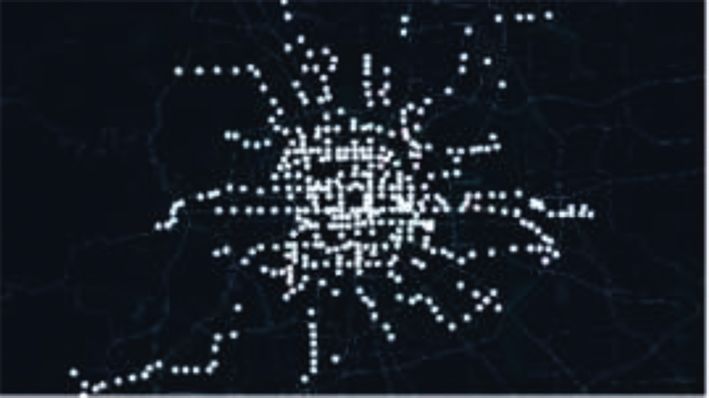
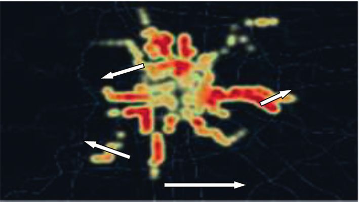
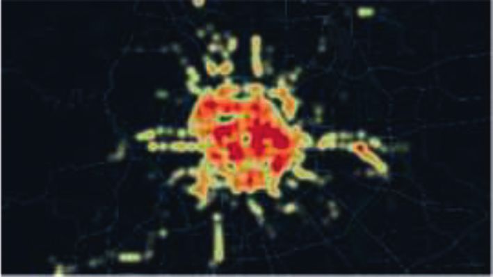
Journal of Advanced Transportation 9

 All trip vectors in dataset

 Mark all samples as unprocessed
 and set the cluster number to –1

 Take a sample All samples in set N

 Yes

 Has the sample been processed? Take a sample in set N
 No
 Yes
 No

 Mark the sample as processed Has the sample been processed?

 No

 Is this sample a core sample? Mark the sample as processed

 Yes Yes

 Add a new cluster C, the cluster Is this sample a core sample?
 No number is incremented by 1
 Yes
 No
 Add all samples in the
 Add the sample to cluster C and set No
 neighborhood of the sample to set N
 its cluster number to the newly
 added number

 Has the sample been processed?
 Get all sample sets N in the
 neighborhood of the sample No
 Add the sample to cluster C and set
 its cluster number to the newly
 Process all samples in set N added number

 Have all samples been processed? Have all samples in set N been
 processed?
 Yes Yes

 Clustering results Return

 Figure 4: DBSCAN algorithm flowchart.

 First, the weighted POIs are generated by fusing mul- meters of metro stations. It can be seen that the residential
tisource data from Lianjia and Arctiler using the method POIs in Figure 5(b) are more evenly distributed and have a
designed in Section 3.1. A total of 11,382 residential POIs higher density in the urban center. On the contrary, the
were captured from Amap within the influence area of the residential POIs in Figure 5(c) are concentrated in suburban
metro station. Among them, 10927 residential POIs were areas in an extremely uneven manner. The reason for the
successfully matched through the residential area data from above difference is that the residential POIs in the central
Lianjia, indicating that the matching rate reached 96%. As area of the city are mainly hotels, villas, and residential
for building data, a total of 6,887 buildings were captured buildings with few floors, while that in the suburban areas
from Amap. Among them, 6336 buildings were correctly are mainly high-density, multistory residential communi-
matched through the Arctiler datasets, indicating a 92% ties. Furthermore, 4 high-density residential areas can be
match rate. It can be found that although there are some clearly observed in Figure 5(c), which are located in the
matching failures, the matching rates were higher than 90%, north, east, and southwest of the city. Comparing existing
which proves that the proposed method can effectively studies, it can be found that the above regions correspond to
weight the original POI data into weighted POIs. Residential Changping, Tongzhou, Fangshan, and Daxing, respectively
POIs are used as examples to illustrate the advantages of [42–44]. The above areas have similar characteristics, such as
weighted POI data, as shown in Figure 5. Among them, low housing prices, high housing density, and a large
Figure 5(a) shows the distribution of Beijing metro stations, number of commuters living in the area. It shows that
while Figures 5(b) and 5(c), respectively, show the distri- weighted POI data can more accurately reflect the categories
bution heat map of raw POIs and weighted POIs within 500 of land use around metro stations.

10 Journal of Advanced Transportation

 (a) (b)

 Changping Tongzhou

 Fangshan

 Daxing

 (c)

Figure 5: Comparison of weighted POIs and raw POIs. (a) The distribution of metro stations. (b) The distribution of raw POIs within
500 meters of metro stations. (c) The distribution of weighted POIs within 500 meters of metro stations.

 Second, the spatiotemporal semantics are embedded 0.05
using the SAE-based framework in Section 3.2. Figure 6
shows how the MSE changes with the number of iterations 0.04
 Mean squared error

when training the SAE model. It can be seen that when the
 0.03
number of iterations reaches 40, the value of MSE remains
stable. That is, SAE can encode the spatiotemporal features 0.02
of the input trip records in a stable way, transforming the
high-dimensional sparse vectors into low-dimensional 0.01
dense vectors.
 Third, the dense trip vectors are clustered using 0
DBSCAN algorithm to realize the mobility pattern recog- 0 20 40 60 80 100 120 140 160 180 200
 Epoches
nition. Since the number of clusters is not manually specified
but is automatically generated according to the parameters δ Figure 6: Changes in MSE during training SAE.
and ε, it is necessary to check the number of clusters and
algorithm performance corresponding to different values of
 ε, and SC is shown in Figure 7. From a global perspective, SC
parameters. This paper aims to identify passenger mobility
 increases with the increase of parameters δ and ε. When δ
patterns, so the number of clusters is required not to be too
 reaches 16 and ε reaches 9.5, the value of SC decreases with
large (difficult to explain the potential activities of passen-
 the increase of parameters. Combining the above two in-
gers) or too small (difficult to distinguish passenger cate-
 dicators, a parameter combination of δ � 16 and ε � 9.5 is
gories) in order to balance practicality and interpretability.
 selected. Herein, SSE � 23715 and SC � 0.815, showing
Through pre-experiments, we found that the number of
 good clustering performance.
clusters decreases as δ and ε increase. Further, when δ < 8
and ε < 7, the number of clusters is verified to be greater than
30, which makes it difficult to accurately describe the po-
tential activities represented by each mobility pattern. When 4.2. Results Analysis. The mobility pattern is recognized
δ > 18 and ε > 10, the number of clusters is less than 3, which using the proposed method with the above parameters.
is obviously not conducive for our exploration of passenger Figure 8 shows the results when δ � 16 and ε � 9.5. Each
mobility patterns. Therefore, the parameter value range is color represents a recognized mobility pattern and C1–C6
determined as: δ ∈ [8, 18] and ε ∈ [7, 10]. Figure 2 lists means the mobility features of cluster 1 to cluster 6. Among
several results of the number of clusters and algorithm them, Figures 8(a) and 8(b) show the distribution of POI
performance quantified by SSE and SC under different categories around the origin station and that around the
parameter values. It can be found that the value of SSE destination station, which reveals the spatial features. The
decreases with the increase of δ, and the influence of ε on SSE distributions of the start time of the day, the distribution of
is limited. The relationship between SC and parameters is the day of week, and the distribution of travel time are
more complicated. Furthermore, the relationship between δ, presented in Figures 8(c)–8(e), respectively.

Journal of Advanced Transportation 11

 0.8
 0.8

 0.6 0.6

 SC
 0.4 0.4
 0.2
 0.2
 10
 9 8 16 18
 7 10 12 14
 ε 8
 δ
 Figure 7: The value of SC corresponding to different parameters.

 Entertainment Entertainment
 0.5 0.5
 0.4 0.4
 Government Working Government Working
 0.3 0.3
 0.2 0.2
 0.1 0.1
 Hospital Shopping Hospital Shopping
 0 0

 Residential Transportation Residential Transportation

 Education Education
 C1 C4 C1 C4
 C2 C5 C2 C5
 C3 C6 C3 C6
 (a) (b)
 5-6 Monday
 23-24 0.35 6-7
 0.64
 22-23 0.28 7-8
 0.48
 0.21 8-9 Sunday Tuesday
 21-22
 0.14 0.32
 20-21 9-10
 0.07 0.16
 0
 19-20 10-11 0

 Saturday Wednesday
 18-19 11-12

 17-18 12-13

 16-17 13-14
 15-16 14-15 Friday Thursday
 C1 C4 C1 C4
 C2 C5 C2 C5
 C3 C6 C3 C6
 (c) (d)
 Figure 8: Continued.

12 Journal of Advanced Transportation

 0-20
 0.6

 0.45

 100-120 0.3 20-40

 0.15

 0

 80-100 40-60

 60-80
 C1 C4
 C2 C5
 C3 C6
 (e)

Figure 8: Six mobility patterns recognized by the proposed method when δ � 16 and ε � 9.5. (a) POI categories around the origin station.
(b) POI categories around the destination station. (c) The start time of the day. (d) The day of week. (e) Travel time.

 The characteristics of the six mobility patterns identi- mobility pattern. wherein it is difficult to directly identify
fied above are summarized, as shown in Table 2. Among the purpose of travel, where the origin location is mainly
them, C1 and C5 account for 35.808% (13.716% + 22.092%), entertainment, shopping, and hospital POIs, the start time
representing the work-related mobility during the work- is between 11 am and 5 pm, and the travel time is within
days. More specifically, C1 reveals long-distance working 40 min. The travel purpose of this pattern is difficult to be
mobility, where the start time is between 7 and 8 am, and accurately identified, but it can be regarded as a short-
travel time is mainly 40–80 min. In contrast, C5 represents distance travel that occurs during off-peak hours on
short-distance working, where the start time is between 7 weekdays.
and 9 am (later than the start time in C1), because travelers The above analysis shows that mobility patterns related
need to spend short travel time (mainly within 40 min). It to working and home are the easiest to identify and explain,
can be found that although the temporal information is in which is consistent with the conclusions of existing studies
line with the typical mobility patterns of commuters, the [23, 45, 46]. On the one hand, according to multidimen-
POIs around the destination station include multiple sional temporal features, work-related mobility patterns can
categories (not only working), such as entertainment, be divided into long-distance mobility and short-distance
working, hospital, and shopping, which characterize the mobility. In this case, the number of short-distance travelers
various possible work places of passengers. Besides, C3 is 1.611 times (22.092%/13.716%) that of long-distance
(accounting for 13.908%) shows entertainment and travelers, which shows that a large percentage of commuters
shopping activities that mainly take place on weekends due work close to their places of residence. Nevertheless, there
to the large number of entertainment and shopping POIs are still many commuters living far away from their working
surrounding the destination station. The start time of this places, reflecting a serious imbalance between working and
type of mobility is between 9 am and 7 pm, and the travel housing [43, 44]. On the other hand, home-related mobility
time is within 60 min. Correspondingly, C2 and C4 account patterns encompass more categories, because travelers can
for 34.323% (19.817% + 14.506%), revealing the home-re- choose the time to go home more freely than the time to
lated mobility, most of which occurs on weekdays and work. Taking C2 and C4 as examples, trips related to going
Sundays. It can be seen that the destination POIs are mainly home are clearly divided into two patterns. The start time of
residential. The difference is that the start time of the C2 is after 5 pm, and that of C4 is mainly between 5 and 7
mobility represented by C2 is all after 5 pm, while that pm. It can be inferred that the start time of the traveler’s
represented by C4 is mainly concentrated between 5 pm home trip is related to their work. In addition to working
and 7 pm. In C2 and C4, the various types of POIs (en- and going home, activities related to entertainment and
tertainment, working, shopping, etc.) around the origin shopping are displayed in C3. Most of them appear on
station represent passengers at different working locations. weekends and their start time is between 9 am and 7 pm,
Finally, C6 (accounting for 15.961%) represents a kind of which shows that passengers are more casual in choosing

Journal of Advanced Transportation 13

 Table 2: Characteristics of mobility patterns.
 Spatial features Temporal features
 Proportion
ID The start The day of Possible activity
 (%) The origin station The destination station Travel time
 time week
 Mainly entertainment,
 Mainly Mainly Mainly 40 Working (long
C1 13.716 Mainly residential POIs working, hospital, and
 7–8 weekdays min–80 min distance)
 shopping POIs
 Mainly entertainment,
 Weekdays Home (short
C2 19.817 working, shopping, and Mainly residential POIs After 17 Within 40 min
 and Sundays distance)
 education POIs
 Mainly residential, Mainly entertainment and Mainly Entertainment
C3 13.908 9–19 Within 60 min
 entertainment POIs shopping POIs weekends and shopping
 Mainly entertainment,
 Mainly Weekdays Mainly 40 Home (long
C4 14.506 working, and shopping Mainly residential POIs
 17–19 and Sundays min– 80 min distance)
 POIs
 Mainly entertainment,
 Mainly Mainly Mainly within Working (short
C5 22.092 Mainly residential POIs working, shopping, and
 7–9 weekdays 40 min distance)
 POIs
 Mainly entertainment, Mainly entertainment,
 Mainly Mainly within
C6 15.961 shopping, and hospital shopping, and residential Weekdays Others
 11–17 40 min
 POIs POIs

start time when engaging in entertainment and shopping 4.3. Sensitivity Analysis of Parameters. In this section, the
activities. The above phenomenon is consistent with our sensitivity of parameters on the recognition results is ana-
empirical observation [18, 23]. It should be noted that the lyzed. As shown in Table 3, the parameters of the clustering
current analysis is based on the parameter settings of δ � 16 algorithm have a significant impact on the recognition per-
and ε � 9.5. When the number of clusters decreases, several formance. Here, we show the results when δ � 14 and ε � 10
work-related patterns may be merged. Conversely, when the in Figure 9 and that when δ � 8 and ε � 10 in Figure 10. In
number of clusters increases, more mobility patterns may be Figure 9, the trip vectors are divided into 3 patterns,
found, but the difficulty of interpreting the pattern recog- SSE � 23647, and SC � 0.793. Obviously, it reveals the three
nition results also increases. most basic patterns of urban mobility: working, home, and
 It should be noted that sometimes the spatial infor- others. Among them, C2 describes working-related trips,
mation of the clustering results is confusing. For example, where the start time is mainly from 7 am to 9 am on weekdays,
both clusters C1 and C3 have trips from residential POI to and the POIs around the origin station are mainly residential.
shopping POI. Nevertheless, C1 and C3 are interpreted as Correspondingly, C3 represents trips related to going home,
different potential activities (long-distance working/enter- where the start time is mainly after 5 pm on weekdays, and the
tainment and shopping). This reflects the uncertainty of POIs around the destination station are dominated residential
identifying passenger mobility patterns only through spatial POIs. In addition, C3 represents trips that include enter-
information and the necessity of using spatiotemporal in- tainment, shopping, etc., where the start time is mainly
formation jointly. For trips with the similar spatial infor- distributed between 10 am and 5 pm on weekends. In Fig-
mation, temporal information can assist in inferring ure 10, the passenger trip vectors are identified as 11 clusters,
mobility patterns. Passengers who intend to shop are un- SSE � 23133 and SC � 0.712. Compared with Figure 8, it can
likely to choose to travel during the morning peak hours. be seen that more passenger activities are identified.
They tend to choose off-peak hours to avoid crowded Among them, C1, C9, and C11 are the three most easily
conditions and obtain higher travel comfort. It can be explained patterns. They characterize working-related trips.
inferred that passengers in C1 who travel during the In more detail, travel time of C1 is mainly 60–80 min, while
morning rush hours with shopping POIs as destinations are that of C9 is within 40 min, and that of C11 is mainly
composed of most of the staff working in the mall and a 20–60 min. The travel time reflects the length of the
small number of shoppers. Conversely, in C3, the potential journey. The three clusters C3, C8, and C10 represent
activity of passengers traveling on weekends with shopping home-related mobility. Their proportions are 13.606%,
POIs as destinations is more likely to be shopping. When 7.478%, and 7.555%, respectively. In detail, the start time of
classifying a passenger’s mobility pattern, the proposed C3 is mainly 5 pm–7 pm, while that of C8 is 7 pm–10 pm,
embedding method can be used to embed the passenger’s and that of C10 is mainly 6 pm–8 pm. This shows that
spatiotemporal information into a low-dimensional vector passengers are more flexible in time selection when going
space. The distance between the embedded vector and the home. The remaining clusters represent mobility other than
vector of each cluster center can be calculated to obtain the working and home, which are a refinement set of C3 and C6
most likely mobility patterns and reduce the confusion in Table 2. Obviously, the mobility represented by these
caused by spatial information. clusters is more dispersed in POI categories and more free

14 Journal of Advanced Transportation

Table 3: The number of clusters and algorithm performance based identify passenger mobility patterns, respectively. We ex-
on different parameters. amine the performance with different vector forms when the
ID δ ε K SSE SC number of clusters is 6. It should be noted that after many
 pre-experiments, when sparse vectors are used and the
1 8 7 27 33136 0.466
2 8 7.5 29 33407 0.473 number of clusters is 6, the input parameters are δ � 22 and
3 8 8 24 30895 0.439 ε � 72. The comparison results are shown in Table 4. It can
4 8 8.5 18 34989 0.139 be seen that the calculation time using sparse vectors is much
5 8 9 16 31018 0.621 longer than that using dense vectors. This is because dense
6 8 9.5 15 31731 0.568 vectors need to consume less computing resources in the
7 8 10 11 23133 0.712 calculation process. In addition, compared to sparse vectors,
8 10 7 24 28931 0.248 using dense vectors can give better results, showing a smaller
9 10 7.5 22 29168 0.38 SSE and a larger SC. The reason is that the SAE-based
10 10 8 19 27447 0.421 embedding method efficiently extracts the spatiotemporal
11 10 8.5 14 27925 0.361
 information in passenger travel records, which proves the
12 10 9 13 27374 0.616
13 10 9.5 12 28828 0.621
 necessity and superiority of embedding spatiotemporal
14 10 10 9 27158 0.657 semantics.
15 12 7 19 26676 0.295 Next, we compare the performance of different methods.
16 12 7.5 17 26224 0.379 Here, two baseline methods are selected from the existing
17 12 8 16 26786 0.424 studies. The first one is a cluster-based method from liter-
18 12 8.5 11 26077 0.188 ature [22]. Different from this paper, this method aims to
19 12 9 11 26775 0.614 mine the spatiotemporal travel patterns from the long-term
20 12 9.5 10 26596 0.56 historical travel database, whereas OD stations are regarded
21 12 10 6 26638 0.686 as spatial features and the timestamps of entering and exiting
22 14 7 18 25702 0.356 stations are regarded as temporal features. The second
23 14 7.5 16 24084 0.381
 baseline method is a topic model based on LDA from lit-
24 14 8 12 25114 0.503
25 14 8.5 10 23429 0.597 erature [23]. In this model, the four features are considered
26 14 9 9 23796 0.646 to describe a passenger trip—they are the location (station),
27 14 9.5 9 23889 0.596 start time of day, start day of week, and the duration. It
28 14 10 3 23647 0.793 should be noted that this model is a “soft-cluster” method,
29 16 7 18 24333 0.348 where a probability distribution is used to quantify the
30 16 7.5 14 22281 0.38 relationship between a trip and mobility patterns.
31 16 8 10 23117 0.502 Due to the lack of real activity labels for passenger travel
32 16 8.5 10 23255 0.487 records, it is challenging to quantify and compare the
33 16 9 9 23760 0.646 performance of various methods in mobility pattern rec-
34 16 9.5 6 23715 0.815
 ognition in terms of accuracy. One way to deal with this
35 16 10 5 23568 0.596
36 18 7 17 22439 0.151
 problem is to design a stated preference (SP) survey to
37 18 7.5 13 21892 0.364 determine the actual travel purpose of passengers, which
38 18 8 10 23129 0.25 can be utilized as a benchmark to calculate the accuracy of
39 18 8.5 7 22538 0.507 the mobility pattern recognition results [47]. Nevertheless,
40 18 9 7 23407 0.681 SP surveys often require huge manpower and material
41 18 9.5 7 23436 0.629 resources, especially in large-scale analysis. In this section, a
42 18 10 6 23675 0.654 compromise method is adopted to evaluate the perfor-
 mance of models by using the SSE calculated by equation
in the start time, which is in line with the diversified (13) and the SC calculated by equation (14). These two
characteristics of weekend entertainment activities. Inev- indicators can measure the ability of the pattern recogni-
itably, as the number of clusters increases, the interpretability tion results to characterize the distribution of the data,
of the results is weakened. For example, there is no significant evaluating the models without real activity labels [23].
difference in the proportion of each category of POI around the Based on the data in Section 4.1, the number of clusters is
origin station and the destination station in C4, which makes it set to 3, 6, and 11 respectively, and the above two methods
difficult to find a known activity to explain its spatiotemporal are used to recognize mobility patterns. Figure 11 shows the
characteristics. A feasible method is to investigate the purpose values of the two indicators (SSE and SC) corresponding to
of the passengers in C4 to explain the above phenomenon. In the results obtained by different methods, in which the K
summary, there must be a trade-off between the number of represents the number of clusters. It can be found that
clusters and interpretability of the results. when the number of cluster is 3 and 6, the SSE of baseline 2
 and that of the proposed method are relatively small, while
 that of baseline 1 is larger. When the number of clusters is
4.4. Comparison of Methods. First, we compare the results 11, the three methods have comparable SSE. This means a
with different vector forms. Here, sparse vectors (50 di- significant intra-cluster difference of identified mobility
mensions) and dense vectors (8 dimensions) are used to patterns when the OD stations are regarded as the spatial