Bus Travel Time Prediction: A log-normal Auto-Regressive (AR) Modeling Approach
←
→
Page content transcription
If your browser does not render page correctly, please read the page content below
Bus Travel Time Prediction: A log-normal Auto-Regressive
                                                           (AR) Modeling Approach

                                                  B. Dhivyabharathi1 B. Anil Kumar2 , Avinash Achar3 , Lelitha Vanajakshi4 *

                                          ABSTRACT
                                          Providing real-time arrival time information of the transit buses has become inevitable in ur-
                                          ban areas to improve the efficiency of the public transportation system. However, accurate
                                          prediction of arrival time of buses is still a challenging problem in dynamically varying traffic
                                          conditions especially under heterogeneous traffic condition without lane discipline. One broad
arXiv:1904.03444v1 [stat.AP] 6 Apr 2019

                                          approach researchers have adopted over the years is to divide the entire bus route into sections
                                          and model the correlations of section travel times either spatially or temporally. The proposed
                                          study adopts this approach of working with section travel times and developed two predictive
                                          modelling methodologies namely (a) classical time-series approach employing a seasonal AR
                                          model with possible integrating non-stationary effects and (b) linear non-stationary AR ap-
                                          proach, a novel technique to exploit the notion of partial correlation for learning from data to
                                          exploit the temporal correlations in the bus travel time data. Many of the reported studies did
                                          not explore the distribution of travel time data and incorporated their effects into the modelling
                                          process while implementing time series approach. The present study conducted a detailed anal-
                                          ysis of the marginal distributions of the data from Indian conditions (that we use for testing in
                                          this paper). This revealed a predominantly log-normal behaviour which was incorporated into
                                          the above proposed predictive models. Towards a complete solution, the study also proposes
                                          a multi-section ahead travel time prediction algorithm based on the above proposed classes
                                          of temporal models learnt at each section to facilitate real time implementation. Finally, the
                                          predicted travel time values were corroborated with the actual travel time values. From the re-
                                          sults, it was found that the proposed method was able to perform better than historical average,
                                          exponential smoothing, ARIMA, and ANN methods and the methods that considered either
                                          temporal or spatial variations alone.

                                          Keywords: Travel time prediction, time-series analysis, partial correlation, non-stationary, log-
                                          normal distribution, multi-section ahead prediction.
                                             1 Doctoral Student, Department of Civil Engineering, Indian Institute of Technology Madras, Chennai, INDIA
                                          600036, E-mail: gebharathi@gmail.com
                                             2 Senior Project Officer, Department of Civil Engineering, Indian Institute of Technology Madras, Chennai,

                                          INDIA 600036, E-mail: raghava547@gmail.com
                                             3 Research Scientist, TCS Innovation Labs, Chennai, INDIA 600113, E-mail: achar.avinash@tcs.com
                                             4 *Corresponding Author, Professor, Department of Civil Engineering, Indian Institute of Technology Madras,

                                          Chennai, INDIA 600036, E-mail: lelitha@iitm.ac.in

                                                                                                1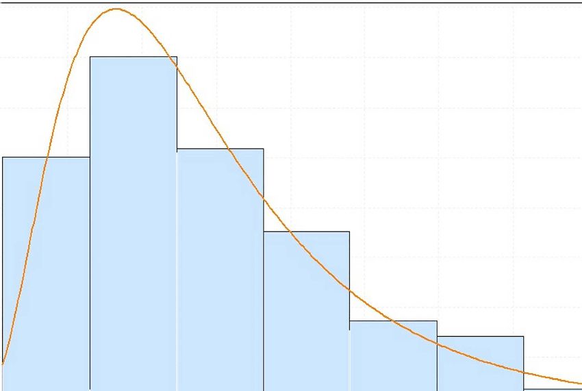
1   INTRODUCTION

Real-time bus arrival information is highly sought-after information in recent years to enhance
the efficiency and competitiveness of public transport [1]. However, uncertainties in arrival time
are quite common in public transit due to dynamic traffic conditions, particularly for highly
varying heterogeneous traffic condition, contributed by various factors such as lack of lane
discipline, fluctuating travel demand, incidents, signal timing and delay, bus stop dwell times,
seasonal and cyclic variations, etc. In countries such as India in particular, public transport
buses scarcely stick to any predefined schedule while bus commuters hardly have any real-time
information of the likely arrival time of the bus they are expecting. Given the lack of this crucial
real-time information, commuters may end up taking private vehicles to reach their respective
destinations. This may lead to reduction in modal share of public transport and increase in
composition of private vehicles contributing towards the raise in congestion and other related
negative impacts. Hence, prediction of travel/arrival time and informing the same to passengers
is inevitable to make public transport more attractive, efficient, and competitive especially in
urban areas. Such real-time information can also be used to assist commuters in making better
trip-related decisions ahead of the journey, which significantly reduces anxiety levels while
waiting for a bus [2, 3, 4]. Thus, it is evident that the negative impacts associated with lack of
reliability of the existing public transportation system can be reduced to an extent by predicting
accurate arrival time of buses and communicating it to the passengers in advance.
     The travel time prediction methodologies can be broadly grouped into data driven and traf-
fic flow theory based methods. With the advent and implementation of diverse modern sensing
technologies that generate large amount of data, data-driven techniques are getting more pop-
ularity. For example, these days, many urban public transportation systems deploy Automated
Vehicle Location (AVL) systems like Global Positioning System (GPS) to monitor the position
of buses in real time, which can provide a constantly growing database of location and tim-
ing details [5]. Such data can rightly be used for developing a Bus Arrival Time Prediction
(BATP) system , as the collected data inherently capture the nature and patterns of traffic in
real time. Many researchers have explored the modelling and prediction of bus travel time,
but only a few studies have considered exploiting the temporal correlations in the AVL data
systematically while also taking into consideration the statistical distributions followed by the
travel time data. This work tries to bridge this gap in existing literature appropriately using
linear statistical models.
     The dynamic bus travel time prediction problem considered in this paper is to accurately
predict the travel times at sections ahead from the current position of the bus as the trip is in
progress in real time. To achieve this, exploiting the information of the travel times experienced
by the previous buses in the subsequent sections is a promising choice. This means utilizing
the temporal dependencies in the spatio-temporal AVL data of all the buses. Hence, the travel
times experienced at different time intervals of the day at a particular section were chosen as

                                                 2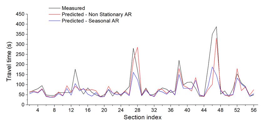
observations of our time series or univariate sequential data. A statistical sequential predic-
tive model using a novel linear, non-stationary approach that performs learning exploiting the
notion of partial correlation is developed. This study also proposes a time-series approach em-
ploying a seasonal AR model with possible integrating non-stationary effects for the prediction
of bus travel time. Both the temporal predictive modelling approaches predict ahead in time
at each segment independently. To appropriately and correctly utilize these temporal predic-
tions available at each section, the present study additionally formulated a multi sections ahead
prediction framework to facilitate real time implementation of the developed BATP system.
    The present study also carried out a detailed analysis of the marginal distributions of the
travel time data collected from typical Indian conditions (that we use for testing in this paper)
which revealed a predominantly log-normal behaviour. The lognormal nature of the data is
incorporated into both the above predictive models and statistically optimal prediction schemes
in the lognormal sense are utilized for all predictions. Our experiments clearly revealed superior
predictions in favor of prediction models which explicitly utilized the lognormal nature of the
data.

2   Literature Review

Various studies have been reported on prediction of travel times and the methods used can be
broadly classified into traffic flow-theory based and data-driven methods.
    Traffic flow theory based methods establish a mathematical relationship between appro-
priate variables that tries to capture the system characteristics. Such methods develop models
based on traffic flow theory, which is mostly based on the first principles of physics. Such
theory-based approaches usually focus on recreating the traffic conditions in the future time
intervals and then deriving travel times from the predicted traffic state [6]. Such theory based
models can be classified as a) Macroscopic, b) Microscopic, and c) Mesoscopic, based on
the level of detail it captures [7, 8, 9, 10]. Majority of the studies under this category used
the conservation of vehicle principle to predict travel time under homogenous traffic condition
[11, 6] and a few studies developed simulation approaches [12], dynamic traffic assignment
based methods [13] for the same. However, all of the above studies predicted travel times from
flow/speed measurements under homogenous traffic conditions. It is very standard to use a
suitable estimation/prediction tool to predict the traffic state variables recursively in real time,
when model based methods are implemented. Most of the studies for travel time prediction
used Kalman Filtering Technique (KFT) as the estimation tool [14, 15, 16, 17, 18, 19]. A few
studies have explored some non-linear estimation tools such as Particle Filtering, Extended
Kalman Filtering, Unscented Kalman Filtering, etc. for the purpose of travel time prediction
[7, 20]. Due to the non-linearity, complexity, and uncertainty of contributing factors of the
traffic conditions, traffic flow theory based methods needs highly complex and sophisticated
models and recursive techniques to capture the system dynamics under high variation condi-

                                                 3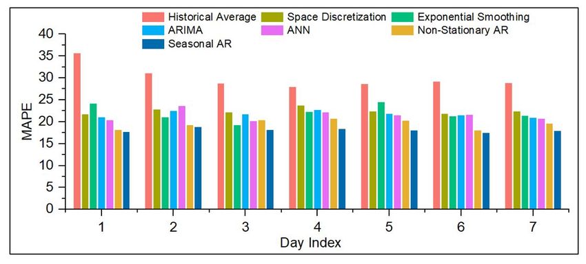
tion.
     Data driven approaches use larger databases to develop statistical/empirical relations to
predict the future travel time without really representing the physical behavior of the modelled
system [21]. In a way, these methods exploit the available data to extract the system charac-
teristics. Various data driven approaches reported in the literature include historical averaging
methods, empirical methods, statistical methods, and machine learning methods.
     Historic averaging methods [22, 23] predict the current and future travel time by averaging
the historical travel time of previous journeys. These methods assume that traffic patterns are
cyclical and the projection ratio (the ratio of the historical travel time in a particular link to the
current travel time) will remain constant. Hence, historic averaging methods are not suitable
for highly varying traffic conditions, where travel times experience large variations.
     Empirical models are based on intuitive empirical relation or mathematical concepts. A few
studies [24, 25, 26, 27, 28, 29, 30] have explored and showed the superiority of the empirical
model combined with recursive filtering over the other methodologies. However, the efficiency
of the method is highly dependent on the presumed relationship or assumptions.
     Machine learning techniques such as Artificial Neural Network (ANN) and Support Vector
Machine (SVM) are some of the most commonly reported prediction techniques for travel
time prediction because of their ability to solve complex relationships [31, 32]. A few studies
[24, 33, 34, 35] combined the machine learning techniques such as SVM, ANN with filtering
algorithms such as Kalman Filtering to predict travel time. [36] and [37] have compared the
performance of ANN and SVM and reported that SVM outperforms ANN in the prediction of
arrival times and also it was reported that SVM is not susceptible to the over fitting problem
unlike traditional ANN, as it could be trained through a linear optimization process. Many
studies [33, 36, 38, 39, 40] have reported better performance of machine learning techniques
compared to other existing methods. However, machine learning techniques require a large
amount of data for training and calibration, and are computationally expensive, restricting their
usage for wide real time applications.
     Statistical methods such as regression and time series predicts the future values by devel-
oping relationship among the variables affecting travel time or from the series of data points
listed in time order. A few studies have implemented regression methods [41, 42, 43, 44, 45,
46, 47, 48, 49, 50] for arrival time prediction. [51] integrated regression methods with adaptive
algorithms to make it suitable for real time implementations. However, the accuracy of the pre-
diction using this approach highly depends on identifying and applying suitable independent
variables. This requirement limits the applicability of the regression model to the transportation
areas as variables in transportation systems are highly inter-correlated [52]. However, the effect
of multicollinearity can be reduced by two approaches – by calculating the value of Variance
Inflation Factor (VIF), or use robust regression analysis instead of ordinary least squares regres-
sion, such as ridge regression [53], lasso regression [54], and principal component regression
[55]. Statistical learning regression methods such as regression tree [56], bagging regression

                                                  4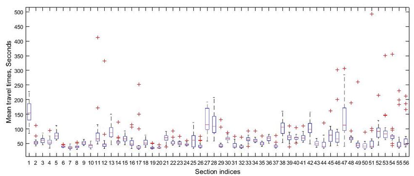
[57], and random forest regression [54] are also used.
     Time series models (or data-driven approaches in general) are based on the assumption that
the current and future patterns in data largely follow patterns similar to historically observed
data. [58] stated that this method greatly depends on historic data to develop relations for
forecasting future time variations. Travel time prediction domain has seen numerous time
series works with various modelling strategies and techniques. Earlier studies [59, 60, 61,
62, 63] estimated travel time from other traffic flow variables such as traffic volume, speed, and
occupancy collected from location-based sensors such as loop detectors and implementations
reported were mainly on freeways.
     Literature has also seen time series appraoches for travel time prediction by modelling
several other related variables such as delays [64], headways [65], dwell time [66], running
speed [67], etc. Only a few studies modelled the travel time observations directly for a BATP
problem. In addition, most of those studies considered either entire trip travel time [68] or bus
stop to bus stop travel time [64], which eventually may not capture the variations in travel time,
if the considered stretch is very long. The present study adopted an effective way of segmenting
the entire route into smaller sections of uniform length. The time-series observations in the
proposed method are different from all these existing time series approaches for analysing bus
travel time data. At each section, the travel times experienced at different times of the day are
modelled as a separate time series. Hence, the proposed approach can potentially capture the
variations in travel time better than earlier methods.
     In a traffic system, the travel times also exhibit patterns which are mostly cyclical with
variations in magnitude depending on the spatial and geometric features of the location. For
example, presence of a signal at a particular location mostly results in higher travel times and
therefore, this trend/pattern would clearly reflect in the historical travel time data. Hence,
the present study adopted a time series (or sequential modelling) framework on travel time
observations at different times of the day for bus arrival time prediction. For each section, the
proposed methodology models the temporal correlations between travel times experienced at
different times of the day. These temporal correlations are learnt using two approaches: (i)
based on a novel application of the notion of partial correlation and (ii) using a seasonal AR
time-series approach.

Studies under Heterogeneous Traffic Conditions: A few methodologies were developed to
predict bus travel time under heterogeneous lane-less traffic condition and are discussed here
[45, 17, 18]. Majority of the above studies used a space discretization approach to predict bus
arrival times [17, 69]. Here, the route was spatially discretized into smaller sections and hy-
pothesized a relation in travel time between neighbouring sections, i.e., the travel time of a bus
in a particular section can be predicted using the travel time of the same bus in the previous
section. This was adopted mainly due to the lack of availability of a good historic data base.
[18] extended the work by separating dwell times and running time from total travel time and

                                                5
modelled their characteristics independently. They found that considering dwell times does not
bring a significant improvement in overall prediction accuracy. However, such a method may
not be able to capture correlations meaningfully in all scenarios. For example, the travel times
in neighbouring sections may not be dependent on each other if one had a signal and the other
is not influenced by that signal. In such cases, prior travel time information from the same
section may be a better input for prediction than the neighbouring section’s travel time. [19]
hypothesized a relation based on temporal evolution of travel time and [10] developed a model
based approach to explore the spatio-temporal evolutions in travel time. Irrespctive of the mod-
elling nature, the aforementioned studies neither analysed nor incorporated the distributional
aspects of travel time into predictive modelling. The current study incorporates this feature
into the predictive model by exploiting the predominantly lognormal nature of the data before
exploring two sequential modelling approaches to model travel time evolutions across the day
to predict bus arrival times.
    This paper is organized as follows. First, the details of study site and data processing
are presented. Next, the section on data analysis discusses the various analysis conducted
to assess the characteristics and variations of travel time. This is followed by methodology
section that explains the travel time prediction schemes developed to incorporate the identified
characteristics of the data using the concepts of time series analysis. Results section is presented
next discussing the evaluation of the proposed approaches using real-world data. Finally, the
study is concluded by summarizing the findings.

3   DATA COLLECTION

Probe vehicles fitted with GPS units are commonly used to collect data for advanced public
transportation system applications. In the present study, data were collected using permanently
fixed GPS units in Metropolitan Transport Corporation (MTC) buses in the city of Chennai,
India. In this study, MTC bus route 19B was considered, which has a route length of around 30
km as shown in Figure 1. The selected route has 25 bus stops and 14 signalized intersections,
many of which are severely congested and oversaturated. The study stretch represents typical
heterogeneous, lane-less Indian traffic and includes varying geometric characteristics, volume
levels, and land use characteristics. The selected route covers both urban and rural areas and
has both four-lane and six-lane roads. The Average Daily Traffic (ADT) at one location with
a counting station in the selected route was measured to be around 40,000 vehicles. Because
of lack of availability of any other counting stations along the route, this number can be con-
sidered as a representative value. The vehicle composition in this stretch is reported to be 47%
two-wheelers, 7.3% three-wheelers, 43.7% light motor vehicles (LMVs), and 2% heavy motor
vehicles (HMVs) [70]. In the test bed identified, there are no exclusive lanes for the public
transport buses. They share the road space with all other vehicle modes. The average headway
between successive buses is around 20 minutes for the selected route. While overtaking of

                                                 6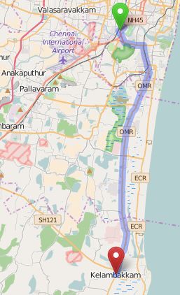
buses is feasible, overtaking of a bus by the next bus of the same bus route is very rare.

                      Figure 1: Study stretch considered (19B bus route).

     In this study, 34 days of GPS data collected at every 5 seconds was used. Out of these
34 days, the last one week’s data were kept for corroboration purpose while the remaining 27
days’ data were use for model building. The collected GPS data included the ID of the GPS
unit, time stamp, and the location details of the bus in terms of latitude and longitude at every
5 seconds. The raw data obtained from GPS were then sorted and checked for quality. This
included trip identification, data processing and data cleaning. Trip identification is the process
through which multiple trips made by a bus in a particular day were separated. This process
also involved the separation of onward and return journeys of the same trip. Data processing
involved conversion of the raw location details (latitude and longitude) into distance, using
Haversine formula [71]. The difference between time stamps of two consecutive GPS data
points gives the travel time for the distance between the selected two points. After this process,
the data consisted of travel times and the corresponding distance between consecutive locations
for all the trips. In this study, the entire route was divided into smaller sections of 500 m length
as it is the average distance found between two successive bus stops and analyses were carried
out. Data cleaning was carried out to remove outliers from the data. The outliers were identified
by assuming free flow speed of 60 km/h as the maximum speed leading to the lower bound of
travel time as 30 s for a 500 m section. The upper bound was kept as 95th percentile travel time
for sections. Travel times less than lower bound and more than upper bound were replaced with
its bound permissible values. After all these steps, the final data set consisted of the date, time,
and 500 m section travel times for every trip.

                                                 7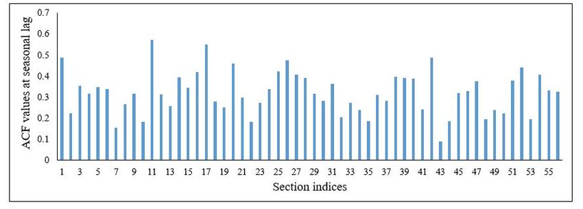
4 PRELIMINARY DATA ANALYSIS
In this study, at each section, the travel times observed at different times of the day are viewed
as sequential data or a time series. The entire 24 hr time window is divided into one hour slots.
Due to absence of data for about 5 hours in the night, we have 19 active slots per day. The
data is pre-processed such that at each time slot there is only one travel time observation. It
was assumed that there are correlations between travel times of adjacent time slots and our
proposed predictive modelling strategies to be explained in the next section precisely capture
this.
Understanding the underlying data distribution is a key step before applying any statistical
modelling approach [72]. The processed data observations were grouped section-wise and dis-
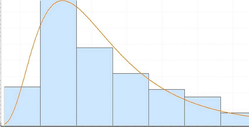
tribution fitting was carried out for each section. An analysis of travel time distribution was
carried out and a few sample histograms are shown in Figure 2. From Figure 2 it can be seen
that the distribution is skewed to the right, which indicate a positively skewed distribution. The
present study used the data distribution fitting software “Easyfit” to check the possible distri-
butions to be tested. In the next level, codes were written in MATLAB to check the distribution
fitting and the subsequent analysis confirmed the selection of lognormal distribution as the best
fit distribution for the considered dataset. In order to check the log-normality of the data, a
Kolmogorov-Smirnov test (K-S test) was conducted at 5% significance level. The null hypoth-
esis assumed for this test is that the data follows log-normal distribution. For majority of cases,
the test failed to reject null hypothesis by showing p-values greater than 0.05, indicating that the
data sets can be approximated by log-normal distribution. Figure 3 shows the results obtained
from K-S test, i.e., p-values for various sections along the route across all hours and days and
Figure 4 shows sample plots of the best log-normal fit for the respective empirical distributions
of Figure 2.
8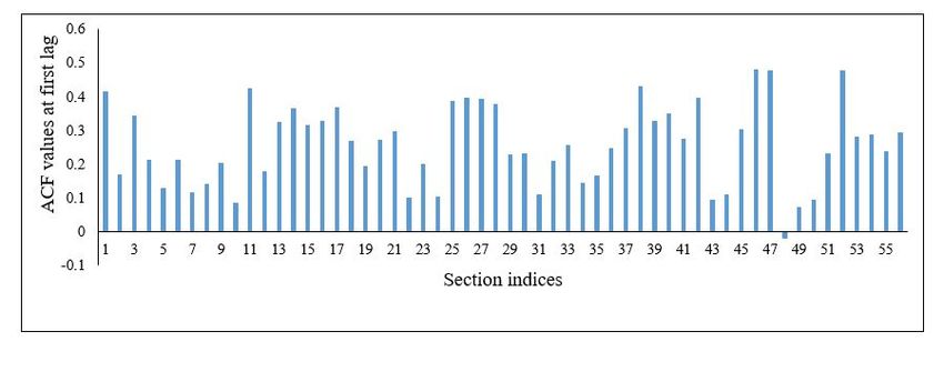
(a) Section 13                        (b) Section 20

            (c) Section 31                        (d) Section 45

                 Figure 2: Histogram for sample sections.

Figure 3: p-values obtained from K-S test for each section across the route.

                                     9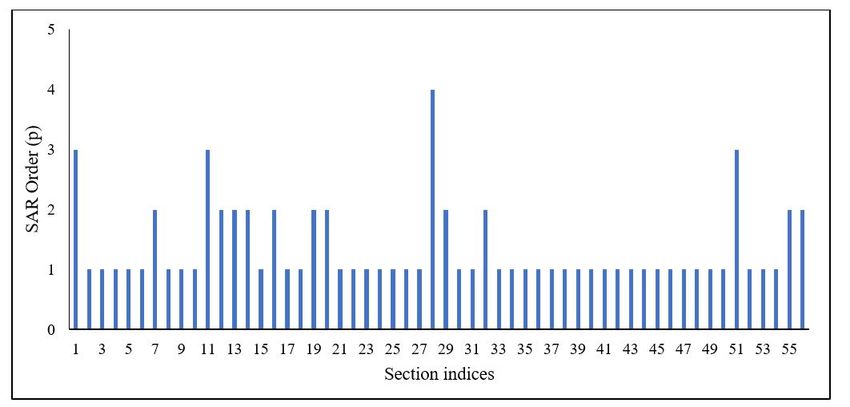
0.4                                                                                                    0.32

     0.36
                                                                                                               0.28

     0.32
                                                                                                               0.24
     0.28
                                                                                                                   0.2
     0.24

                                                                                                          x0.16-
    � 0.2-                                                                                                ..__..         .

     0.16-                                                                                                     0.12-

     0.12-                                                                                                     0.08

     0.08
                                                                                                               0.04
     0.04
                                                                                                                    0
          0
                    60        80           100               120          140       160        180                           30        32    34   36         38          40         42       44     46         48    50   52
                                             Travel time (x), seconds                                                                                             Travel time (x), seconds

                                    ID Histogram      -Log normal I                                                                                    ID Histogram       -Lognormal I

                                    (a) Section 13                                                                                                 (b) Section 20

     0.36                                                                                                      0.32

     0.32                                                                                                      0.28

     0.28                                                                                                      0.24

     0.24
                                                                                                                   0.2

    x   0.2-                                                                                               X
                                                                                                          �0.16-
     0.16-
                                                                                                               0.12-
     0.12-
                                                                                                               0.08
     0.08
                                                                                                               0.04
     0.04
                                                                                                                    0
          0
               32        36    40        44             48           52     56     60     64                                      40        60     80              100            120         140        160        180   200
                                              Travel time (x), seconds                                                                                            Travel time (x), seconds

                                    ID Histogram      -Lognormal I                                                                                          ID Histogram - Lognormal I

                                    (c) Section 31                                                                                                 (d) Section 45

                                       Figure 4: Distribution fitting results for sample sections.

    As the analysis results showed that the marginal distribution of data is mostly log-normal,
the next stage was to model this data, incorporating its log-normal characteristics. The present
study adopts concepts of time series to design prediction schemes under log normal data distri-
bution assumption, which is described in the next section.

5       METHODOLOGY

    As described in the previous section, a KS test showed lognormal distribution as the best fit
among a set of standard distributions for modelling the marginal distribution of the data. The
pdf of a univariate lognormal random variable Y with parameters µ and σ is defined as

                                                                                                 1     (ln(y)−µ)2
                                                                                                     −
                                                                                 fY (y) =        √ e       2σ 2   ,                                                                                                            (1)
                                                                                               xσ 2π

where ln(Y ) is a Gaussian random variable with mean µ and variance σ 2 . Accordingly, the
travel time observations are assumed to follow a lognormal process. Prediction schemes, which
exploit the lognormality exhibited by the data and make statistically optimal predictions are
proposed. This study explores temporal modelling and prediction in primarily two ways. In the
first approach (Seasonal AR modelling), the non-stationarity of the data is tackled by removing

                                                                                                     10
possible deterministic trends and seasonality in the data before applying standard stationary
model fits. In the second approach (Non-stationary method), a general non-stationary data-
driven model with a principled method to estimate the time-varying parameters of the non-
stationary model is proposed. In these proposed approaches, both the Gaussian and log-normal
assumptions on the data are explored and are disscussed below.
5.1 Seasonal AR Modelling with Possible Integrating Effects
A classical (Gaussian distribution based) time series approach for modelling and learning based
on historical data and subsequent prediction is explained here. Towards the end of the section,
we discuss how the lognormality of the data can be incorporated into the approach based on
Gaussian assumptions. Data from about 27 days was used for training or model fitting. Each
day’s travel time observations (19 of them) at each section were concatenated together (in the
order of dates) to form a single long time series.
Compensating for standard non-stationarities, if any: In time series analysis, it is a standard
practice to first filter out deterministic non-stationarities like (polynomial) trends and periodic-
ities (also refered to as seasonality sometimes) from the data (which is usually non-stationary)
before applying standard stationary model fits. On visual inspection, it was observed that there
are no linear or higher order trends in the time series of any section. Further, on inspection of
the Auto Correlation Function (ACF) (sample plots shown in Figure 5), no abnormally slow
decay of the ACF was found at consecutive lags. Presence of polynomial trends in the data
typically manifests in a slowly decaying ACF which is not the case in our data. Figure 6 shows
the ACF values at lag 1 (which are all significantly less than 1) in all the sections to ascertain
this. Please observe that the lag 1 ACF values at all sections are significantly less than 1, which
rules out the presence of polynomial trends. Further, since the data has been constructed by
stringing together short time series segments of a fixed length (19 in this case), it is natural to
check for periodic (seasonal) trends of period one day. The presence of a deterministic seasonal
component can manifest itself in the ACF again with a slow decaying trend at the seasonal lags.
Figure 7 shows the ACF values at seasonal lag and it can be seen that the values are signif-
icantly less than 1 in all the sections. Hence, there was no evidence of presence of periodic
(seasonal) trends in our data and it was concluded overall that deterministic non-stationarities
are absent in the data.
Among the stochastic types of non-stationarity, the well-known integrating type effect was
checked using the ADF unit-root test. We have conducted the ADF test at the optimal lag
length to ascertain the presence of unit-root stochastic non-stationarities in the data. First, the
maximum lag length for the sample was obtained using Schwert’s thumb rule [73] and ADF
test was conducted for all lag lengths. Then, lag length with lowest BIC value is identified
as optimal lag length and the corresponding ADF test results were considered for the decision
making. In the present study, the ADF test rejected the null hypothesis for all the sections. The
11integrating type stochastic non-stationarity can occur at a seasonal level too. The ACF decay
at seasonal lags being significantly less than 1 is one clear evidence to rule out the presence of
seasonal unit roots. Figure 7 which shows the ACF values at the first seasonal lag demonstrates
that the decay factor is significantly less than 1 in all the sections. This rules out the presence
of seasonal unit roots.
(a) Section 12 (b) Section 45
Figure 5: Sample ACF plots for selected sections of the route
Figure 6: ACF values at first lag for all the sections.
Seasonal AR model fit: On the conditionally (if the unit-root test detected integrating effects)
differenced data, the ACF and Partial Auto Correlation Function (PACF) is computed. It was
observed that in all cases PACF decayed quickly (shown in Figure 8). This condition is an ideal
candidate for a pure AR model fit [74]. Moreover, prediction is a very simple process under
AR model fits. Even though the ACF decays considerably after a couple of initial lags, it again
picks up (statistically) significant magnitude at the intial seasonal lags (specifically at 19 here).
This indicates that even though there are no deterministic seasonal components that repeat in a
fixed fashion, there do seem significant correlations (stochastic) between travel times exactly a
day apart (19 ticks here). To incorporate this expected and important feature of the ACF, this
study propose to use a seasonal AR model with an appropriately identified model order using
12Figure 7: ACF values at first seasonal lag for all the sections.
(a) Section 12 (b) Section 45
Figure 8: Sample PACF plots for selected sections of the route.
its PACF. It is standard in time series to fix the AR-model order based on the significant PACF
co-efficients. This study explores the usage of (a) Multiplicative Seasonal AR Model and (b)
Additive Seasonal AR Model. A multiplicative seasonal AR model for a process y(t) is of the
form
(1 − φ1 L − φ2 L2 − · · · − φ p L p )(1 − Φ1 Ls − Φ2 L2s − · · · − Φk LPs )y(t) = e(t), (2)
where, e(t) is a white noise process with unknown variance, L p is the one-step delay operator
applied p times i.e. L p y(t) = y(t − p). As the name multiplicative suggests, the AR term in the
stationary process is a multiplication of two lag polynomials: (a) first capturing the standard
lags of order upto p, (b) second capturing the influence of the seasonal lags at multiples of the
period s and order upto P. For instance, for the PACF shown in Fig 8a, the choice of order
parameters would be p = 2, P = 1, and s = 19. An additive seasonal AR model on the other
hand is a conventional AR model (1 − φ1 L − φ2 L2 − · · · − φ p L p )y(t) = e(t) with co-efficients
corresponding to the insignificant values in the PACF constrained to be zero. For instance,
for the PACF shown in Figure 8a, an AR model of order 19 is chosen with co-efficients φ3 to
φ18 forced to zero. Both the multiplicative and additive seasonal AR models are learnt using
13maximum likelihood estimation [75]. We finally choose the model with the higher AIC between
these two for prediction. Figure 9 shows the order p of the learnt AR model at every section.
Also, this study stuck to one seasonal lag (P = 1) for building the overall SAR model.
Figure 9: Seasonal AR model order (p) across all the sections.
Incorporate log-normality: Our first proposed scheme is based on stationary log-normal
AR modelling [76]. A log-normal stationary AR process (Y1 ,Y2 , . . . ) is one whose transformed
process (X1 , X2 , . . . ) obtained by applying log on each of its random variables is a stationary
Gaussian AR process. This means (Xi = ln(Yi )), ∀ i. As shown in [76], if one is predicting Yn
based on its past values Y1 ,Y2 . . .Yn−1 , then the conditional distribution of Yn is also log-normal
with parameters µ = ∑ki=1 wi ∗ Xn−i and σ 2 . Here wi , i = 1, . . . k are the AR parameters and σ 2
is the variance of the input noise, both in the associated Gaussian AR process. Accordingly
we apply a log transformation on all the travel time observations first, and then fit an AR
model as explained above. While predicting, in case the data is differenced due to presence of
integrating type effects, one needs to do linear prediction on the differenced data and finally
undo the differencing after linear prediction. We finally apply the exponential transformation to
obtain the actual travel time prediction. Applying an exponential transformation is equivalent to
choosing the median of the conditional log-normal distribution as the final point estimate which
is statistically optimal under the mean absolute error loss function [77]. Log-normal modelling
(unlike Gaussian modelling) gives us the flexibility of trying out the mean and mode (which are
optimal under the mean square error and ε-insensitive loss functions [77] as well apart from the
median (all three of which are distinct) for the final point estimates. Both these point estimates
additionally would need the conditional variance of the prediction in the Gaussian domain.
145.2 Linear Non-Stationary Approach
The classical time series approach discussed before assumes the data to be a sum of possi-
ble trend and periodic (deterministic) non-stationarities plus a stochastic stationary component
(with possible integrating type stochastic non-stationarities). The next approach that is dis-
cussed here, on the other hand models the data in a non-stationary fashion directly. The con-
ventional time-series approach (discussed before) assumes one long realization of a random
process. It assumes ergodicity of the process for estimating ensemble averages using time aver-
ages [75]. However, the non-stationary model we now consider involves a fixed finite number
of random variables. The number of random variables in this random vector will be equal to the
number of slots we bin the 24 hr axis into, at each section. To learn the statistics of these finite
set of random variables, one needs independent and identically distributed (i.i.d.) realizations
of this finite-dimensional random vector. The travel time vector (at a fixed section) of a partic-
ular day which consists of observations from different time-bins of the day can be regarded as
one realization of this random vector. The collection of all such travel time vectors across all
training days constitute i.i.d. realizations of this random vector.
Recall from Figure 6 of the previous (SAR) subsection that we did not find any trend in the
travel time sequential (time-series) vector which was obtained by concatenating all the daywise
travel time training vectors in order. This justifies our assumption to regard the daywise travel
time vectors at a particular section to be identically distributed. However, this joint distribution
can change from section to section. Presence of a trend in the day-wise concatenated time series
would nullify our assumption that these day-wise travel time vectors are identically distributed.
Hence, it can be assumed that these 27 travel time vectors as i.i.d and estimate the joint
distribution of these 19-dimensional random vector at each section separately. Before we pro-
ceed to fit a predictive model, we first look at the empirical mean of each of these 19 random
variables at every section. We provide the mean variation plot at two randomly chosen sections
across the 19 time bins in Figure 10. We further provide a box plot of the mean travel times
in a day across all the 56 sections in Figure 11. This overall justifies the evidence for (mean)
non-stationarity at each section amongst these 19 random variables.
15(a) Section 27 (b) Section 47
Figure 10: Variation of mean travel time across time intervals of the day
Figure 11: Box plot of mean travel time across sections.
Motivated from this observation, the proposed approach tries to fit a general Gaussian/ log-
normal model to aid real-time predictions based on the travel-time of the past time-bins of
the same day. We propose to use a non-stationary auto-regressive modelling approach, which
makes prediction a straightforward and computationally inexpensive task. Firstly, the non-
stationary AR-model is explained under the Gaussian assumption. Extending it further under a
log-normal joint distribution is similar to the stationary log-normal AR case.
As the name auto-regressive suggests, the proposed model assumes that any travel time ob-
servation can be obtained by linearly regressing a finite set of preceding past values. In partic-
ular, any travel time observation Xn (at time-bin n) can be written as a linear combination (with
a bias) of a set of its k(n) immediately preceding values plus some independent Gaussian noise
with an unknown time-varying (n-dependent) variance. This form of non-stationarity brings
in two levels of generality as opposed to a stationary Gaussian AR process: (a) The regressing
weights now would be a function of n, (b) The number of immediately preceding past (travel-
time) values that influence at time-bin n can also vary with n i.e. the weight vector length k(n)
16is now a function of n. We denote the weight vector at time bin n as wn = [wn0 , wn1 , wn2 , . . . wnk(n) ].
Figure 12 illustrates these non-stationarity influences.
w35
w25 w27
w15 w16 w17
X1 X2 X3 X4 X5 X6 X7
w26
w37
1 2 3 4 5 6 7
TimeBin Index
Figure 12: Illustration of non-stationary model: Influences on to a particular time bin indicated
via arcs of the same color and associated weights wni (except wn0 ) at time bin 5, 6 and 7. k(5) = 3,
k(6) = 2, k(7) = 3.
At each section, the sequence of travel time observations of each historical day is consid-
ered a realization of the above non-stationary process. For each section, the entire collection
of all historical (27) days is treated as (27) i.i.d realizations from this process. The availability
of i.i.d. data from many days in the historical past makes estimation of the time-varying re-
gression weight vectors wn = [wn0 , wn1 , wn2 , . . . wnk(n) ] feasible for each time-bin n. The estimation
process can be a little tricky given that the length of the weight vector is not known apriori.
The problem boils down to solving the following statistical conditional independence question:
Given the recent past k values upto time n − k, are the current and the past beyond time (n − k)
conditionally independent? If this is the case, the main advantage is as follows. To predict the
current travel time Xn , knowledge of only its k past values are necessary and one can forget
about the past beyond (or before) Xn−k . We are in particular interested in the least such k for
which this holds. Checking this conditional independence for general distributions can be com-
plicated or even infeasible. However for Gaussian distributions, the notion of partial correlation
(PC), comes to our aid here, which is defined as follows.
Partial correlation as the name suggests captures the correlation between those parts of A
and B that are not explainable by C. Interestingly, for multi-variate Gaussian distributions,
it turns out that the conditional independence between A and B given C holds if and only if
the associated PC between A and B given C is 0 [78], as stated next. This crucial relation
is what facilitates a method to ascertain the necessary conditional independence to build our
non-stationary auto-regressive model.
Definition 1. [79, 80] Given random variables A and B and a random vector C = (C1 ,C2 , . . .Cn ),
the partial correlation between A and B given C is defined as the correlation coefficient between
residual errors eA = (A − f1 (C)) and eB = (B − f2 (C)), where f1 (C) is the optimal linear pre-
dictor (in the mean square sense) of A given C and f2 (C) is the optimal linear predictor (in the
mean square sense) of B given C.
17Property 1. Consider random variables X and Y and a random vector Z such that (X,Y, Z)
are jointly Gaussian. X and Y are conditionally independent given Z if and only if the partial
correlation between X and Y is zero.
Proof. For Gaussian joint distributions, all conditional distributions are also Gaussian with
mean being a linear function of the conditioning random variables while the variance is con-
stant and independent of the values assumed by the conditioning random variables [81]. This
means the joint distribution of X and Y (conditioned on Z) would be Gaussian. It is an ele-
mentary fact that independence of two jointly Gaussians is equivalent to their covariance being
zero. Hence, checking for conditional independence of X and Y is equivalent to checking for
their conditional covariance being zero. Checking for conditional variance being zero for every
value of the conditioning random variables is in general computationally infeasible. However,
in the joint Gaussian case, one can show that the conditional variances and conditional cor-
relation co-efficients are independent of the specific values the conditioning random variables
can assume [82]. This means that the conditional covariance which is the product of condi-
tional variance and conditional correlation co-efficient will be independent of the conditioning
random variables.
The linear regressor of X w.r.t. Z i.e. the best linear approximation of X in terms of Z in
the mean-square error (MSE) sense is E(X/Z) when X and Z are jointly Gaussian. For similar
reasons, the linear regressor of Y w.r.t Z is E(Y /Z). Hence in the multi-dimensional Gaussian
setting, the partial correlation can be written as
E [(X − E(X/Z))(Y − E(Y /Z))] (3)
Z
= E [(X − E(X/Z))(Y − E(Y /Z))/Z = z] fZ (z)dz
Z
= E [(X − E(X/Z = z))(Y − E(Y /Z = z))/Z = z] fZ (z)dz,
the first term in the above integral is the conditional covariance between X and Y which is
independent of z as explained above. Hence this constant term can come out of the integral and
PC is now equal to this constant conditional covariance. Hence the property follows.
Algorithm 1 gives a detailed explanation of computing the order and values of auto-regression
and the additive noise variance for a specific time bin n. The algorithm basically computes the
sample partial correlation (PC) between Xn and Xwin−1 given all the intermediate random vari-
ables namely (Xn−1 , Xn−2 , . . . Xwin ) for win varied progressively from n − 1 to 2 (line 2). For a
particular win, it performs a forward regression to compute wf , the optimal linear predictor of
Xn in terms of (Xn−1 , Xn−2 , . . . Xwin ) (line 3). Similarly, it performs a backward regression to
compute wb , the optimal linear predictor of Xn in terms of (Xn−1 , Xn−2 , . . . Xwin ) (line 4). The
associated residual errors of both the forward and backward linear regressions are computed
next (lines 5 to 7). As per definition 1, sample PC is computed by calculating the correla-
tion coefficient of the rf and rb (line 10). To statistically ascertain if the computed sample PC
18Algorithm 1: Learn/Estimate AR Co-efficients and Noise Variance at Each Time Bin
n for a Fixed Section.
Input: Historical Data D = [x1 x2 . . . xT ](d×S) , S - total no. of time bins in the day. d -
number of days for training, xi (d×1) - travel time observation vector at the ith
time bin of the day.
Output: wn = [wn0 , wn1 , wn2 , . . . wnk(n) ], σn2 .
1 Initialize Flag = 1;
2 for win ← (n − 1) to 2 do
3 Linearly regress Xn w.r.t (Xn−1 , Xn−2 , . . . Xwin ) to obtain wf with INPUT =
(xn−1 , xn−2 , . . . xwin ), OUTPUT = (xn ).
4 Linearly regress Xwin−1 w.r.t (Xn−1 , Xn−2 , . . . Xwin ) to obtain wb with INPUT =
(xn−1 , xn−2 , . . . xwin ), OUTPUT = (xwin−1 ).
5 From wf and wb , compute the respective sample residuals rf and rb , as below:
6 ∀i, rf (i) ← xn (i) − ∑n−win f f
j=1 w ( j) ∗ xn−j (i) + w (0), i - day index.
7 ∀i, rb (i) ← xwin (i) − ∑n−win b b
j=1 w ( j) ∗ xn−j (i) + w (0), i - day index.
8 Compute ParCor, sample correlation coefficient between rf and rb .
9 /* The above computes partial Correlation between Xn & Xwin−1 given the
intermediate random variables (X , X , . . . Xwin ). */
√n−1 n−2
∗ ParCor d−2
10 Compute test statistic t ← 1−ParCor2 to assess if ParCor == 0 based on a
standard t-test ([82]).
11 if p-value of t ∗ > 0.05 then
12 Flag = 0 ;
13 break;
14 if Flag == 1 then
15 Linearly regress Xn w.r.t (Xn−1 , Xn−2 , . . . X1 ) to obtain wf with INPUT =
(xn−1 , xn−2 , . . . x1 ), OUTPUT = (xn ).
16 Compute sample residual rf from wf .
2
17 σn ← Sample variance of rf ;
f
18 return (w , σn )
2
is zero or not, we use hypothesis testing. In particular, our null hypothesis used is PC equal
to zero. We employ
√
a standard t-test [82] for assessing zero correlation coefficient with test
ParCor d−2
statistic 1−ParCor2 (line 10) which is known to follow a t-distribution with d − 2 degrees of
freedom. If the p-value of the test statistic is less than 0.05 (significance level), we reject the
null-hypothesis. Note that the test is 2-sided with the test statistic possibly taking both positive
and negative values. We stop at the earliest instance of win where p-value is greater than 0.05
(line 11 to 13). This means we retain the null hypothesis and the partial correlation is assessed
to be zero. This would give us the order of autoregression, k(n) = (n − win) at time bin n. This
is also the minimum number of previous travel times conditioned on which the current Xn and
the past (Xwin−1 and beyond) are independent. If the PC is not significantly close to zero for
any win, then Xn is dependent on the entire past (lines 16 and 17).
Incorporating lognormality: A lognormal non-stationary AR process can be defined as
one whose log-transformed process is a Gaussian non-stationary AR process. Learning under
19this model, can be readily achieved by first taking the log of all the observations and then fitting
a gaussian non-stationary AR model as explained above.
The optimal prediction for the Gaussian non-stationary AR model at time tick n given
k(n)
the current past (X1 , X2 . . . Xn−1 ) is carried out as X̂(n) = wn0 + ∑i=1 wni ∗ Xn−i . In the lognor-
mal case, the original current observations (Y1 ,Y2 . . .Yn−1 ) are log transformed first to obtain
(X1 , X2 . . . Xn−1 ). The optimal linear combination in the Gaussian domain is computed like ear-
k(n)
lier X̂(n) = wn0 + ∑i=1 wni ∗ Xn−i and the final optimal point estimate in the lognormal domain
is Ŷ (n) = expX̂(n) . This point estimate turns out to be the median of the conditional distribution
P(Yn /Yn−1 ,Yn−2 . . .Y1 ), which is also lognormal. One can also use the mean and mode of this
conditional lognormal distribution for a point estimate in which case we would additionally
need information of σn2 (in addition to X̂(n)). However for the purposes of the current paper
we stick to the median which translates to the use of a simple exponentiation of the prediction
in the Gaussian domain.
5.3 Real-time prediction across multiple sections ahead
In the previous two subsections, linear statistical models (with lognormality incorporated while
not necessarily stationary) which capture temporal correlations in the bus travel time data were
proposed. The temporal prediction models built at each section need to be ultimately used for
real-time predictions of travel times for a bus whose trip is currently active. The constructed
models can predict temporally ahead into the future at every section. However, what we need
is predicting travel times of a currently plying bus over a couple of sections ahead of its current
position. It is not immediately clear how the sequential prediction models developed in the
previous sections could be used for travel-time prediction over a subroute of arbitrary sections
ahead from the current position of an active bus.
We illustrate the method via an example as shown in the space-time diagram of Figure 13.
We assume that the time bins are all of the same duration of one hour even though our proposed
methodologies can be used for general non-uniform time bin durations. The bus is currently on
the verge of leaving current section i (i = 2 here). The current time is 2 : 30 PM with the current
time bin j = 11 in this example. We assme that the current real-time information is available
on these various subsequent sections upto the previous time bin ( j − 1 = 10). The current (or
observed) real-time travel time information at a subsequent section a and time bin b is denoted
a,pr
as Tba,ob , while the predicted travel time at a section a and time bin b is denoted as T[b . In the
example, it is further assumed that the learnt models are simple autoregressive models of order
2 for ease of illustration. This means we need real-time data from only the previous two time
bins as the shaded region of the first two rows of the space-time diagram indicates. Prediction
of travel time on one section ahead of the bus’s current position (section 3 in the example) is
pretty straight forward.
Given that the bus is currently just leaving section i at time bin j ( j = 11 in the example), to
202-STEP PREDICTION (Temporal)
Td
10
ex < 5PM
5 PM
1-STEP PREDICTION (Temporal)
13 d
10,pr
T13
Td
7 d8 d9
ex < 4PM Tex < 4PM Tex > 4PM
4 PM
12 d
6,pr d
7,pr d
8,pr d
9,pr d
10,pr
T12 T12 T12 T12 T12
TimeBin Index
Td
4 d5
ex < 3PM Tex > 3PM
3 PM
Tcur =2:30PM
11 d
3,pr d
4,pr d
5,pr d
6,pr d
7,pr d
8,pr d
9,pr d
10,pr
T11 T11 T11 T11 T11 T11 T11 T11
2 PM
3,ob 4,ob 5,ob 6,ob 7,ob 8,ob 9,ob 10,ob
10 T10 T10 T10 T10 T10 T10 T10 T10
1 PM
9 T93,ob T94,ob T95,ob T96,ob T97,ob T98,ob T99,ob T910,ob
1 2 3 4 5 6 7 8 9 10
Section Number
Figure 13: Illustration of the multi-section ahead travel time prediction.
predict the bus’s travel time on section i + 1, one needs to use the current real-time travel time
information on section i + 1 (from all previous buses) upto previous time bin j − 1. One needs
to perform a one-step temporal prediction at section i + 1 to predict the bus’s travel time one
section ahead as shown in Figure 13.
To extend this to an arbitrary number of sections ahead in a principled way, one would need
to potentially perform a multi-step temporal prediction (using either of the sequential models
previously discussed) at the subsequent sections. For a subsequent section `, the larger the
difference between ` and current section i, the number of temporal steps ahead we need to
predict at section ` will proportionately go up. The fundamental idea of the algorithm is as
follows. It sequentially goes through the sections ahead starting from section i + 1. We predict
the travel times based on the temporal model learnt at that section by performing a one-step
prediction to start with. For every travel time predicted at a subsequent section k, we update
the expected exit time of the bus from section k by adding this prediction time. The exit time
thus calculated for section k is also the expected entry time into section k + 1. The first instance
when the expected exit time enters the next time bin (namely j + 1), the temporal prediction
from the next section onwards has to be 2-step ahead. Note that this happens at section 5 in the
illustration of Fig. 13 upto which a single-step prediction is performed to calculate the estimates
[3,pr [ 4,pr [ 5,pr
as clearly indicated via the quantities T11 , T11 and T11 . A 2-step temporal prediction is
adopted from the next section because the current real-time data we have from the previous
21Algorithm 2: Travel-Time Prediction Across k-sections Ahead
Input: Current Real Time Data of all previous buses, Current position of the current
bus at the end of some section i, Current Time Tcur .
Output: Predicted Travel Times to travel k sections ahead from section i + 1 starting at
time Tcur .
1 Compute the current time bin, j within which Tcur falls ;
2 Initialize Tc ex = Tcur ;
3 Initialize TimeStepAheadInd = 1 ;
4 Initialize ExpTimeBin = j ;
5 for k = 1, 2, . . . K do
6 Do TimeStepAheadInd-step temporal linear prediction at section i + k using either
the seasonal AR model OR the non-stationary AR model in the Gaussian domain
(using the log transformed raw data) to obtain T (i+k),pr .
7 /* Predict Travel time at section i + k using the current real time data at section
i + k upto time bin j - 1. */
8 /* In other words, predict travel time for time bin j - 1 + (TimeStepAheadInd) at
section i + k.*/
9 Tcex = T cex + exp(T
(i+k),pr ).
10 if Tcex falls outside ExpTimeBin then
11 TimeStepAheadInd = TimeStepAheadInd + 1;
12 ExpTimeBin = ExpTimeBin + 1;
13 return TravelTime
buses is only upto time bin j − 1, while the bus would reach this subsequent section only in
time bin j + 1. Accordingly from now on, for a consecutive block of sections one performs a
two-step prediction till the first instance the expected exit time moves into time bin j + 2 and
the process continues. In the example, the next such block of sections where 2-step prediction
is carried out ranges from 6 to 9.
Algorithm 2 presents a pseudocode for achieving this. Current time, Tcur happens to fall
in the current timebin, j, numbered 11 with duration 2 pm to 3 pm (line 1). Tc ex captures the
dynamically predicted exit time from a section as the algorithm iterates sequentially through
subsequent sections. TimeStepAheadInd captures the number of time-steps ahead that the tem-
poral models should predict as the algorithm proceeds. TimeStepAheadInd starts with 1 (line
3). ExpTimeBin captures the time bin in which the bus is expected to be as the prediction pro-
ceeds forward sequentially in space. It is as expected initialized to j, the current time bin (line
4). TimeStepAheadInd gets incremented suitably whenever the exit time Tc ex falls beyond the
ExpTimeBin (line 11). ExpTimeBin also gets incremented under the same condition as shown
in line 12. At the kth subsequent section (from section i), we make a TimeStepAheadInd-step
ahead prediction of the temporal model pre-learnt at section i + k (line 6). Fig. 13 clearly
illustrates how the number of temporal steps ahead prediction needed at a section i + k is pro-
portional to k. It starts with a consecutive block of sections on which the temporal models
perform a 1-step temporal prediction followed by the next consecutive block of sections, in
22each of which a 2-step temporal prediction is carried out and so on.
6 RESULTS
The proposed methodologies were implemented in MATLAB for both single step prediction
and multi step prediction and the performance was evaluated in terms of Mean Absolute Per-
centage Error (MAPE) and Mean Absolute Error (MAE). Testing was carried out for a period
of seven days and results are discussed below.
6.1 Performance Evaluation
The present study evaluated the predicted travel time values with the actual measured travel
time values. The evaluation was done at three stages to highlight the observations and contri-
butions of the present study. First part of the study evaluates the log-normal assumptions of
the data by comparing the results of Seasonal AR method and Non-stationary method under
both Gaussian and log-normal assumptions at an aggregate level. Next, the proposed methods
were compared with each other and the inferences were made at section level and trip level to
know the superiority amongst them. Finally, the performance of the multi-step ahead predic-
tion framework was evaluated and compared between the Seasonal AR and the non-stationary
method.
6.1.1 Single step prediction
Exploiting Log-normality assumptions: To begin with, the performance of the proposed
methods under Gaussian and log-normal assumptions were analyzed to check the validity of
log-normal properties of the data by incorporating the same in prediction scheme. Figure 14
show the MAPE values obtained when the proposed methods were implemented under Gaus-
sian and log-normal assumption. Figures clearly show that the predictions are better under
log-normal assumption compared to Gaussian. Hence, it can be concluded that incorporating
log-normal nature of the travel time data in to the modeling process did improve the prediction
accuracy of the proposed methods and hence for further evaluation, the performance of the
methods was analyzed only under log-normal domain.
In the next stage, performance was compared at an aggregate level of the seasonal AR and
non-stationary method with the measured travel times from field. Sample plot of actual and
predicted travel time values for a given trip (during test period) are shown in Figure 15. Figure
clearly shows that the predicted travel time values are closely matching with the actual travel
time values. Though, the performance of both the proposed methods are comparable, it can be
observed that the peak travel time values around are better captured by non-stationary method.
23You can also read