Scientific Basis: Analysis and Projection of Sea Level Rise and Extreme Weather Event - Bappenas
←
→
Page content transcription
If your browser does not render page correctly, please read the page content below
Scientific Basis:
Analysis and Projection of Sea Level Rise
and Extreme Weather Event
AUTHORS
     Indonesia Climate Change Sectoral Roadmap - ICCSR

     Scientific basis: Analysis and Projection of Sea Level Rise and Extreme Weather Events

     Adviser

     Prof. Armida S. Alisjahbana, Minister of National Development Planning/Head of Bappenas

     Editor in Chief

     U. Hayati Triastuti, Deputy Minister for Natural Resources and Environment, Bappenas

     ICCSR Coordinator

     Edi Effendi Tedjakusuma, Director of Environmental Affairs, Bappenas

     Editors

     Irving Mintzer, Syamsidar Thamrin, Heiner von Luepke, Dieter Brulez

     Synthesis Report

     Coordinating Authors for Adaptation: Djoko Santoso Abi Suroso

     Scientific Basis: Analysis and Projection Sea Level Rise and Extreme Weather Event Report

     Author: Ibnu Sofian

     Technical Supporting Team

     Chandra Panjiwibowo, Edi Riawan, Hendra Julianto, Leyla Stender, Tom Harrison, Ursula Flossmann-
     Krauss

     Administrative Team

     Altamy Chrysan Arasty, Risnawati, Rinanda Ratna Putri, Siwi Handinah, Wahyu Hidayat, Eko Supriyatno,
     Rama Ruchyama, Arlette Naomi, Maika Nurhayati, Rachman

                                                                                                        i
ICCSR - Scientific basis: Analysis and Projection of Sea Level Rise and Extreme Weather Events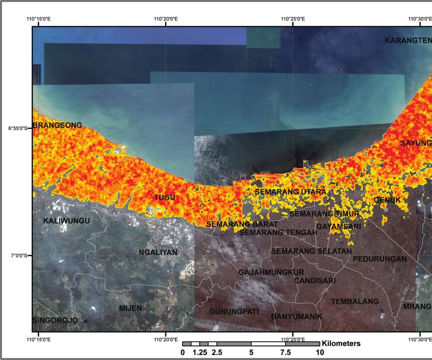
ACKNOWLEDGMENTS
     The Indonesia Climate Change Sectoral Roadmap (ICCSR) is meant to provide inputs for the next five
     year Medium-term Development Plan (RPJM) 2010-2014, and also for the subsequent RPJMN until
     2030, laying particular emphasis on the challenges emerging in the forestry, energy, industry, agriculture,
     transportation, coastal area, water, waste and health sectors. It is Bappenas policy to address these
     challenges and opportunities through effective development planning and coordination of the work
     of all line ministries, departments and agencies of the Government of Indonesia (GoI). It is a dynamic
     document and it will be improved based on the needs and challenges to cope with climate change in the
     future. Changes and adjustments to this document would be carried out through participative consultation
     among stakeholders.

     High appreciation goes to Mrs. Armida S. Alisyahbana as Minister of National Development Planning
     /Head of the National Development Planning Agency (Bappenas) for the support and encouragement.
     Besides, Mr. Paskah Suzetta as the Previous Minister of National Development Planning/ Head of
     Bappenas who initiated and supported the development of the ICCSR, and Deputy Minister for Natural
     Resources and Environment, Ministry of National Development Planning /Bappenas, who initiates and
     coordinates the development of the ICCSR.

     To the following steering committee, working groups, and stakeholders, who provide valuable comments
     and inputs in the development of the ICCSR Scientific basis for Analysis and Projection Sea Level Rise
     and Extreme Weather Events document, their contributions are highly appreciated and acknowledged:

     Steering Committee (SC)

     Deputy of International Cooperation, Coordinating Ministry for Economy; Secretary of Minister,
     Coordinating Ministry for Public Welfare; Executive Secretary, Agency for Meteorology, Climatology;
     Deputy of Economy, Deputy of Infrastructures, Deputy of Development Funding, Deputy of Human
     Resources and Culture, Deputy of Regional Development and Local Autonomy, National Development
     Planning Agency; and Chief of Secretariat of the National Council for Climate Change.

     Working Group

     National Development Planning Agency

     Sriyanti, Yahya R. Hidayat, Bambang Prihartono, Mesdin Kornelis Simarmata, Arum Atmawikarta,
     Montty Girianna, Wahyuningsih Darajati, Basah Hernowo, M. Donny Azdan, Budi Hidayat, Anwar Sunari,
     Hanan Nugroho, Jadhie Ardajat, Hadiat, Arif Haryana, Tommy Hermawan, Suwarno, Erik Amundito,
     Rizal Primana, Nur H. Rahayu, Pungki Widiaryanto, Maraita, Wijaya Wardhana, Rachmat Mulyanda,
     Andiyanto Haryoko, Petrus Sumarsono, Maliki

                                                                                                              iii
ICCSR - Scientific basis: Analysis and Projection of Sea Level Rise and Extreme Weather Events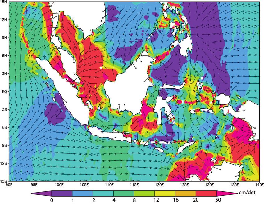
Agency for Meteorology, Climatology and Geophysics

Edvin Aldrian, Dodo Gunawan, Nurhayati, Soetamto, Yunus S, Sunaryo

National Institute of Aeuronatics and Space

Agus Hidayat, Halimurrahman, Bambang Siswanto, Erna Sri A, Husni Nasution

Research and Implementatiton of Technology Board

Eddy Supriyono, Fadli Syamsuddin, Alvini, Edie P

National Coordinating Agency for Survey and Mapping

Suwahyono, Habib Subagio, Agus Santoso

Grateful thanks to all staff of the Deputy Minister for Natural Resources and Environment, Ministry of
National Development Planning/ Bappenas, who were always ready to assist the technical facilitation as
well as in administrative matters for the finalization process of this document.

The development of the ICCSR document was supported by the Deutsche Gesellschaft für Technische
Zusammenarbeit (GTZ) through its Study and Expert Fund for Advisory Services in Climate Protection
and its support is gratefully acknowledged.

iv
                 ICCSR - Scientific basis: Analysis and Projection of Sea Level Rise and Extreme Weather Events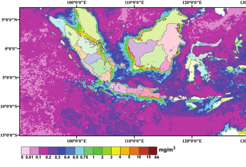
Remarks from Minister of National
       Development Planning/ Head of Bappenas
                                      We have seen that with its far reaching impact on the world’s ecosystems
                                      as well as human security and development, climate change has emerged
                                      as one of the most intensely critical issues that deserve the attention
                                      of the world’s policy makers. The main theme is to avoid an increase
                                      in global average temperature that exceeds 2˚C, i.e. to reduce annual
                                      worldwide emissions more than half from the present level in 2050.
                                      We believe that this effort of course requires concerted international
                                      response – collective actions to address potential conflicting national
                                      and international policy initiatives. As the world economy is now facing
                                      a recovery and developing countries are struggling to fulfill basic needs
                                      for their population, climate change exposes the world population to
                                      exacerbated life. It is necessary, therefore, to incorporate measures to
     address climate change as a core concern and mainstream in sustainable development policy agenda.

     We are aware that climate change has been researched and discussed the world over. Solutions have
     been proffered, programs funded and partnerships embraced. Despite this, carbon emissions continue
     to increase in both developed and developing countries. Due to its geographical location, Indonesia’s
     vulnerability to climate change cannot be underplayed. We stand to experience significant losses. We will
     face – indeed we are seeing the impact of some these issues right now- prolonged droughts, flooding and
     increased frequency of extreme weather events. Our rich biodiversity is at risk as well.

     Those who would seek to silence debate on this issue or delay in engagement to solve it are now
     marginalized to the edges of what science would tell us. Decades of research, analysis and emerging
     environmental evidence tell us that far from being merely just an environmental issue, climate change will
     touch every aspect of our life as a nation and as individuals.

     Regrettably, we cannot prevent or escape some negative impacts of climate change. We and in particular
     the developed world, have been warming the world for too long. We have to prepare therefore to adapt
     to the changes we will face and also ready, with our full energy, to mitigate against further change. We
     have ratified the Kyoto Protocol early and guided and contributed to world debate, through hosting
     the 13th Convention of the Parties to the United Nations Framework Convention on Climate Change
     (UNFCCC), which generated the Bali Action Plan in 2007. Most recently, we have turned our attention
     to our biggest challenge yet, that of delivering on our President’s promise to reduce carbon emissions by
     26% by 2020. Real action is urgent. But before action, we need to come up with careful analysis, strategic
     planning and priority setting.

                                                                                                             v
ICCSR - Scientific basis: Analysis and Projection of Sea Level Rise and Extreme Weather Events
I am delighted therefore to deliver Indonesia Climate Change Sectoral Roadmap, or I call it ICCSR, with the
aim at mainstreaming climate change into our national medium-term development plan.

The ICCSR outlines our strategic vision that places particular emphasis on the challenges emerging in
the forestry, energy, industry, transport, agriculture, coastal areas, water, waste and health sectors. The
content of the roadmap has been formulated through a rigorius analysis. We have undertaken vulnerability
assessments, prioritized actions including capacity-building and response strategies, completed by
associated financial assessments and sought to develop a coherent plan that could be supported by line
Ministries and relevant strategic partners and donors.

I launched ICCSR to you and I invite for your commitment support and partnership in joining us in
realising priorities for climate-resilient sustainable development while protecting our population from
further vulnerability.

				                                           Minister for National Development Planning/

			                                         Head of National Development Planning Agency

                                                      Prof. Armida S. Alisjahbana

vi
                 ICCSR - Scientific basis: Analysis and Projection of Sea Level Rise and Extreme Weather Events
Remarks from Deputy Minister for Natural
        Resources and Environment, Bappenas
                                       To be a part of the solution to global climate change, the government
                                       of Indonesia has endorsed a commitment to reduce the country’s
                                       GHG emission by 26%, within ten years and with national resources,
                                       benchmarked to the emission level from a business as usual and, up to
                                       41% emission reductions can be achieved with international support
                                       to our mitigation efforts. The top two sectors that contribute to the
                                       country’s emissions are forestry and energy sector, mainly emissions
                                       from deforestation and by power plants, which is in part due to the fuel
                                       used, i.e., oil and coal, and part of our high energy intensity.

                                          With a unique set of geographical location, among countries on the
                                          Earth we are at most vulnerable to the negative impacts of climate
     change. Measures are needed to protect our people from the adverse effect of sea level rise, flood,
     greater variability of rainfall, and other predicted impacts. Unless adaptive measures are taken, prediction
     tells us that a large fraction of Indonesia could experience freshwater scarcity, declining crop yields, and
     vanishing habitats for coastal communities and ecosystem.

     National actions are needed both to mitigate the global climate change and to identify climate change
     adaptation measures. This is the ultimate objective of the Indonesia Climate Change Sectoral Roadmap, ICCSR.
     A set of highest priorities of the actions are to be integrated into our system of national development
     planning. We have therefore been working to build national concensus and understanding of climate
     change response options. The Indonesia Climate Change Sectoral Roadmap (ICCSR) represents our long-term
     commitment to emission reduction and adaptation measures and it shows our ongoing, inovative climate
     mitigation and adaptation programs for the decades to come.

                                                 Deputy Minister for Natural Resources and Environment

                                                          National Development Planning Agency

                                                                    U. Hayati Triastuti

                                                                                                              vii
ICCSR - Scientific basis: Analysis and Projection of Sea Level Rise and Extreme Weather Events
LIST OF CONTENTS
AUTHORS                                                                                             i

ACKNOWLEDGMENTS                                                                                    iii

Remarks from Minister of National Development Planning/Head of Bappenas                            v

Remarks from Deputy Minister for Natural Resources and Environment, Bappenas                      vii

LIST OF TABLES                                                                                     x

LIST OF FIGURES                                                                                    xi

LIST OF ABBREVIATIONS                                                                             xv

1 INTRODUCTION                                                                                     1

       1.1   Background                                                                            2

       1.2   Aims and Objectives                                                                   3

2 CLIMATE AND OCEANOGRAPHIC CONDITION IN INDONESIAN SEAS                                   5     2.1
      Wind and Rain Patterns                                                                       6

       2.2   Sea Level Variations                                                                  7

		           2.2.1 Ocean Currents and Sea Level                                                    7

		           2.2.2 Tidal Forcing                                                                  10

		           2.2.3 Significant Wave Height                                                        11

       2.3   The Distribution of Chlorophyll-a and Sea Surface Temperature                        12

3 METHODOLOGY                                                                                     15

       3.1   Data                                                                                 16

       3.2   Method                                                                               17

4 PROJECTION OF SEA LEVEL RISE AND SEA SURFACE TEMPERATURE                                        23

       4.1   Sea Surface Temperature Rise Projection                                              24

       4.2   Sea Level Rise Projection                                                            28

		           4.2.1   Sea Level Rise Projection based on the IPCC AR4                              28

viii
              ICCSR - Scientific basis: Analysis and Projection of Sea Level Rise and Extreme Weather Events
4.2.2 Sea Level Rise Projection (Post-IPCC AR4) 33
5 EL NIÑO AND LA NIÑA PROJECTIONS 39
5.1 Global Warming and ENSO 41
5.2 ENSO and Sea Level Variations 45
5.2.1 ENSO and Mean Sea level 45
5.2.2 ENSO and Extreme Waves 47
5.3 ENSO, Sea Surface Temperature and Chlorophyll-a 51
5.4 ENSO and Coral Bleaching 53
6 ESTIMATION OF INUNDATED AREA 57
6.1 Inundated Area Estimation 58
6.2 Inundated Area Estimation during Extreme Weather Events 61
CHAPTER 7 CONCLUSIONS AND RECOMMENDATIONS 68
REFERENCES 69
ix
ICCSR - Scientific basis: Analysis and Projection of Sea Level Rise and Extreme Weather EventsLIST OF TABLES
Table 4. 1 Projection of the SST increase of Indonesian waters 27
Table 4. 2 Potential source of the sea level rise 27
Table 4. 3 Projection of the average increase of sea level in Indonesian waters 33
Table 5. 1 ENSO timetable based on MRI model output 45
x
ICCSR - Scientific basis: Analysis and Projection of Sea Level Rise and Extreme Weather EventsLIST OF FIGURES
Figure 1. 1 Flow chart of climate change study in support to climate change adaptation 3
action plan
Figure 2. 1 The pattern of wind and sea level temperature (SLT) on January and August 7
Figure 2. 2 Annual cycle of mean rainfall in Indonesia on January and August 7
Figure 2. 3 Spatial distribution of SLH and surface current on January and August. 8
Figure 2. 4 Distribution of sea level and surface current pattern on January and August 9
Figure 2. 5 Spatial distribution of the mean monthly highest tidal range in Indonesian Seas 10
Figure 2. 6 Mean monthly of wave height on January and August. Wave data is taken from 11
altimeter Significant Wave Height (SWH) from January 2006 to December
2008
Figure 2. 7 The spreading pattern of chlorophyll-a on January and August 13
Figure 3. 1 Example of time-series of Sea Level Data from several stations in Indonesia and 17
surrounding area.
Figure 3. 2 Flowchart of sea level rise estimation using historical data and IPCC model, that 18
consist of 4 models, which are MRI, CCCMA CGCM 3.2, Miroc 3.2 and NASA
GISS ER
Figure 3. 3 Climatology of sea level based on tide data, altimeter and model 19
Figure 3. 4 Morlet Wavelet 19
Figure 3. 5 Determination process of Nino3 that is used to estimate the occurrence of El 20
Niño and La Niña
Figure 3. 6 Wavelet analysis result using Nino3 SST data and results for MRI model for 21
SRESa1b scenario
Figure 3. 7 Height of tidal and direction of tidal current at 07.00 WIT before the lowest 21
tide
Figure 3. 8 Speed and direction of tidal current at 07.00 WIT when head to the lowest tide 22
Figure 3. 9 Tide prediction based on 8 main harmonic constants using OTIS model and tide 22
gauge data in Tanjung Priuk in Jakarta
xi
ICCSR - Scientific basis: Analysis and Projection of Sea Level Rise and Extreme Weather EventsFigure 4. 1 Time-series of SST based on paleoclimate data from 150 thousand years ago 24
to 2005, with the highest SST occurring 125 thousand years ago, 30ºC in West
Pacific and Indian Ocean, and 28 ºC in East Pacific (Hansen, 2006)
Figure 4. 2 The trend of SST rise based on the data of NOAA OI, with the highest increase 25
trend occurring in Pacific Ocean in north of Papua, and the lowest in south
coast of Java.
Figure 4. 3 The global trend of SST based upon observation data from 1870 to 2000, with 26
the rate of SST rise reaching 0.4°C/century±0.17°C/century (Rayner, et al.,
2003)
Figure 4. 4 The rate of SST rise based on IPCC SRESa1b, using MRI_CGCM 3.2 model 27
Figure 4. 5 Average sea level rise for 15 years from January 1993 to December 2008, using 28
0 cm as the lowest regional sea level
Figure 4. 6 The average magnitude of sea level from 2001 to 2008 subtracted from the 29
average magnitude of sea level rise from 1993 to 2000, with the varying increase
of sea level between 2 cm and 12 cm, and the average increase of 6 cm, in 7
years.
Figure 4. 7 The trend of sea level increase based on altimeter data from January 1993 to 30
December 2008 using spatial trend analysis
Figure 4. 8 Approximation of sea level rise using a number of tidal data acquired from 31
University of Hawai’i Sea Level Center (UHSLC)
Figure 4. 9 Approximation of global sea level change based on IPCC SRESa1b assuming 31
the CO2 concentration is 750ppm
Figure 4. 10 Approximation of the amount of sea level rise in Indonesian waters based on 32
scenario of IPCC SRESa1b, assuming the CO2 concentration is 750ppm
Figure 4. 11 Positive feedback of ice melting and the rising of surface temperature (UNEP/ 34
GRID-ARENDAL, 2007)
Figure 4. 12 The change in Antarctica’s temperature in the last 30 years 35
Figure 4. 13 The change of the ice-covering layer on Greenland based on analysis using 36
satellite IceSAT (source: Earthobservatory, NASA, 2007)
Figure 4. 14 The sea level rise until year 2100, relative to sea level in 2000 36
Figure 4. 15 Estimated rate of sea level rise in Indonesian waters, based on model projections 37
plus dynamic ice melting, post IPCC AR4
xii
ICCSR - Scientific basis: Analysis and Projection of Sea Level Rise and Extreme Weather EventsFigure 5. 1 An illustration of the scheme and causes of marine transportation accidents 40
in the last few decades. SSH and SST indicates the sea surface height and sea
surface temperature respectively.
Figure 5. 2 Sea level climatology based on tide gauge, altimeter, and IPCC model data. 41
Model data were only displayed by sea level at the southern coast of Lombok
Island.
Figure 5. 3 Result of wavelet analysis for historic data from 1871 to 1998. The dC indicates 42
the degree Celsius
Figure 5. 4 Wavelet analysis results for the SRESa1b scenario. The dC indicates the degree 43
Celsius
Figure 5. 5 Wavelet analysis results for the SRESa2 scenario. The dC indicates the degree 44
Celsius
Figure 5. 6 Wavelet analysis results for the SRESb1scenario. The dC indicates the degree 44
Celsius
Figure 5. 7 Time series of altimeter sea level anomaly from 1993 to 2008. Sea level anomaly 46
falls to 20cm during strong El Niño, and rise 20cm during strong La Niña
Figure 5. 8 Hovmoller diagram of time-latitude sea level anomaly from 1993 to 2008, with 46
lowest sea level anomaly in 1997/1998 during strong El Niño and the highest in
2008 during La Niña
Figure 5. 9 Average of significant wave height processed from altimeter from 2006 to 47
2008
Figure 5. 10 Hovmoller Diagram of daily time-latitude Significant Wave Height (SWH) 48
with the lowest SWH happening in the area at 8°S to 4°N, also SWH height
is inversely proportional between SWH in the South China Sea, Pacific and
Sulawesi Sea (between 4°N to 12°N) with SWH in the Indian Ocean (between
8°S to 12°S)
Figure 5. 11 Maximum significant wave height during extreme wave, processed from the 49
altimeter data of significant wave height from 2006 to 2008
Figure 5. 12 Time-series of wave height from January 1st 2006 to March 1st 2009 in Java 49
Sea
Figure 5. 13 Time-series of wave height from January 1st 2006 to March 1st 2009 in the 50
southern of Java Island
xiii
ICCSR - Scientific basis: Analysis and Projection of Sea Level Rise and Extreme Weather EventsFigure 5. 14 Wind speed and direction on December 29th 2009 51
Figure 5. 15 SST anomaly from 90°E to 150°E and from 15°S to 15°N on August and 52
September year 1980 to 2008. The increase of SST of more than 0.35°C shows
strong La Niña period, and decrease of 0.35°C shows strong El Niño
Figure 5. 16 Chlorophyll-a distribution on September during normal condition, El Niño and 53
La Niña
Figure 5. 17 Estimated locations where massive coral bleaching happens based on the 54
difference of the highest sea level temperature to mean sea level temperature
Figure 5. 18 Coral bleaching sites as a result from SST increase in 1998 until 2006 (Marshall 55
and Schuttenberg, 2006)
Figure 5. 19 Map of coral reef damage and coral bleaching based on data from Basereef. 56
org
Figure 6. 1 Flow chart of process and general method for estimating sea-water-inundated 58
area in year 2100
Figure 6. 2 Estimation of sea-water-inundated area due to influence of sea level rise which 59
reach 1m, subsidence level of 3m per century, and 80cm of tide.
Figure 6. 3 Estimation of sea water-inundated area due to influence of sea level rise that 60
reaches 1m, subsidence level of 2m per century, and 50cm of tide.
Figure 6. 4 Estimation of sea water-inundated area due to the influence of sea level rise that 61
reaches 1m, subsidence level of 2.5 m per century, with highest tide as high as
1.5 m from MSL.
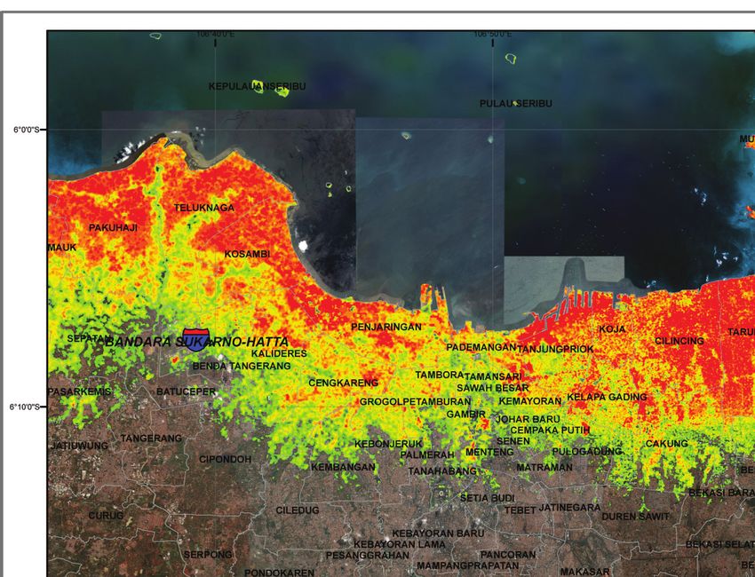
Figure 6. 5 Inundated area in Jakarta in year 2100 during extreme weather 62
Figure 6. 6 Inundated area in Semarang in year 2100 during extreme weather 62
Figure 6. 7 Inundated area in Surabaya in year 2100 during extreme weather 63
xiv
ICCSR - Scientific basis: Analysis and Projection of Sea Level Rise and Extreme Weather EventsLIST OF ABBREVIATIONS
CGCM Coupled General Circulation Model
ENSO El Niño Southern Oscillation
GCM General Circulation Model
GISS Goddard Institute for Space Studies
GHG Green House Gases
HYCOM HYbrid Coordinate Ocean Model
IOSEC Indian Ocean South Equatorial Current
IPCC Intergovernmental Panel on Climate Change
ITF Indonesian Through Flow
MODIS Moderate Resolution Imaging Spectroradiometer
MRI Meteorological Research Institute
NASA National Aeronautics and Space Administration
NOAA National Oceanic and Atmospheric Agency
OI Optimum Interpolation
OTIS Ocean Tidal Inverse Solution
PECC Pacific Equatorial Counter Current
PNEC Pacific North Equatorial Current
PSEC Pacific South Equatorial Current
PTW Pacific Trade Wind
SST Sea Surface temperature
SRES Special Report on Emission Scenario
SRTM Shuttle Radar Topographic Mission
SWH Significant Wave Height
TRMM Total Rainfall Measurements Mission
UHSLC University of Hawai’i Sea Level Center
xv
ICCSR - Scientific basis: Analysis and Projection of Sea Level Rise and Extreme Weather Eventsxvi
ICCSR - Scientific basis: Analysis and Projection of Sea Level Rise and Extreme Weather Events1
INTRODUCTION
1
ICCSR - Scientific basis: Analysis and Projection of Sea Level Rise and Extreme Weather Events1.1 Background
It has been estimated that 23% of the world’s population lives within both 100 km distance from the coast
and less than 100 m elevation above sea level, and population densities in coastal regions are about three
times higher than the global average (Small and Nicholls, 2003). This causes a serious vulnerability to the
sea level rise caused by global warming. Meanwhile, human activities, in general, are believed to be the
biggest contributors to the atmospheric built of greenhouse gases (GHGs), including water vapor (H2O),
carbon dioxide (CO2), methane (CH4), and chlorofluorocarbons (CFCs).
As the global warming process intensifies, the frequency of occurrence and intensity of El Niño and La
Niña also increases (Timmerman et al, 1999). In general, El Niño occurs once in 2-7 years, but since 1970,
the El Niño and La Niña frequency changes to once in 2-4 years (Torrence and Compo, 1999). Moreover,
during El Niño in 1997/1998, Indonesia as a whole experienced a long dry season and during La Niña in
1999, Indonesia experienced a high increase of rainfall, with sea level rise ranging from 20 cm up to 30
cm. This combination of events led to floods in large areas of Indonesia, especially in the coastal region.
Using sea level data on Java Sea from IPCC models, Sofian (2007) Predicted that the frequency of El
Niño and La Niña events will become biennial during the period from year 2000 to 2100.
Aside from extreme climate events (e.g., El Niño and La Niña), global warming also causes sea level rise,
both from the expansion of seawater volume as the result of temperature rise in the ocean and from the
melting of glaciers and polar ice caps in the North and South Pole. Although the impact of sea level rise
is only a subject of discussion among scientists, various climate change studies show that the sea level
rise potential could range from 60 cm up to 100 cm, in year 2100. Regardless as the debate people living
in the coastal area of Indonesia must have a broad awareness of the decrease of life quality in coastal
regions due to sea level rise.
Globally, sea level rise (SLR) is about 3.1mm/year today, while the average sea level rise in the 20th
century is only 1.7 mm/year. More than a third of sea level rise is caused by the melting of icecaps in
the Greenland and the Antarctica, and by the retreat of glacial ice. Some recent research shows that the
melting of glacial and polar ice will increase as global warming intensifies. If the warming and the melting
of ice continue at a rate similar to that of the past 5 years, then the predicted sea level rise in 2100 could
be as much as 80 cm to 180 cm.
The impacts and the consequences of SLR in various coastal regions will be influenced by numerous
factors that interact with one another. These include up-thrusting of the land surface, subsidence, and
coastal plantation conservation as a protection against inundation caused by SLR. Sea Level Rise has the
potential to impact the people living in coastal environments of Indonesia, particularly along the northern
coast of Java island, which is inhabited by more than 40 % of the country’s total population. This risk
creates an urgent need for action on adaptation (as well as mitigation) in order to assist the people who
will face the consequences caused by sea level rise. It is hoped that this study will provide the basic for the
concrete guidance on how best to adapt to the impact and consequences of sea level rise in shoreline and
2
ICCSR - Scientific basis: Analysis and Projection of Sea Level Rise and Extreme Weather Eventscoastal environments. One approach to understanding the correlations among climate change, adaptation
study, and the planning of prudent response strategies are illustrated in Figure 1.1.
Figure 1. 1 Flow chart of climate change study to support
for climate change adaptation action plan
1.2 Aims and Objectives
The aims of this study are as follows:
1. To investigate the SLR rate caused by the global warming.
2. To investigate the impacts of global warming on the sea surface temperature (SST), the intensity of
extreme events and their impacts on the significant wave height characteristics.
Meanwhile, the purposes of this study are:
1. To provide a base reference and information for resilient coastal area development, in order to adapt
to the risks of future climate change, particularly sea level rise (SLR).
2. In addition, by identifying the base reference, adaptation plan for reducing the risks of sea level rise
could be well prepared.
Aside from sea level rise projection, this study will analyze the changing frequency and severity of
extreme events caused by global warming and, in particular, of the effects of global warming to La Niña
and El Niño, which are also referred to as ENSO (El Niño Southern Oscillation). The time-frequency
3
ICCSR - Scientific basis: Analysis and Projection of Sea Level Rise and Extreme Weather Eventsanalysis for extreme events was conducted using wavelet analysis to find the moment and frequency of
occurrences of El Niño and La Niña.
This study is structured as follows: the first chapter contains an introduction that includes the background
and objectives of the study; the second chapter outlines the climate and oceanographic condition of
Indonesian Seas. It covers sea level and surface temperature climatology, chlorophyll-a spatial distribution,
and wave height. The third chapter explains the methodology and the data used for our analysis, while
the fourth chapter presents the projection of sea surface temperature (SST) and sea level. It is followed
by the fifth chapter on ENSO projection, based on sea surface temperature in the Nino3 area (defined
as area between 5°S and 5°N and between 210°E and 270°E), and the analysis of ENSO effects on
the characteristics of sea level, chlorophyll-a spatial distribution, SST, and wave height. The last chapter
contains our conclusions and recommendations for adaptation to the risks of disaster due to sea level rise
caused by global warming and ENSO.
4
ICCSR - Scientific basis: Analysis and Projection of Sea Level Rise and Extreme Weather Events2
CLIMATE AND
OCEANOGRAPHIC
CONDITION IN
INDONESIAN SEAS
5
ICCSR - Scientific basis: Analysis and Projection of Sea Level Rise and Extreme Weather EventsIndonesia is a maritime country located between two oceans, the Indonesian Ocean and the Pacific
Ocean. This unique geophysical position affects the monsoon pattern, rainfall, and other characteristics
of regional climate.
2.1 Wind and Rain Patterns
In the northwesterly wind season from October to March (i.e., when wind blows from the west), the
weather in Indonesia is affected by the northwest monsoon. During this period, the wind blows from the
northeast and turns to the southeast after passing through the equator. By contrast, in the season of the
southeasterly wind from May to September, the wind blows from southeast and turns to northeast after
passing through the equator. The influence of the Pacific Ocean is dominant in the period of westerly
wind (except in most part of Sumatera, which is affected by the western Indian Ocean). Meanwhile
during the season of the easterly wind, the influence of the Indian Ocean is dominant, and is marked
by reduced rainfall on Java Island and in Nusa Tenggara. However, during this period, most parts of
Sumatera and Kalimantan still have high probability of experiencing medium intensity of rainfall.
The propagation of northerly wind from October to March pushes down the warm seawater from the
Pacific Ocean to the Indian Ocean. This causes high rainfall in almost every area of Indonesia. While in
the season of easterly wind from May to September, eastern wind pressure pushes the low temperature
seawater back from the Indian Ocean to the Pacific Ocean through the Java Sea, the Karimata Strait
and the South China Sea. This period is marked by decreasing rainfall in Java, Kalimantan and southern
Sumatera. At the same time, in the Riau Islands, western Sumatera may still have rain due to the high SST
around those areas.
Figure 2.1 shows the wind pattern and spatial distribution of SST in January during the peak of west
wind season and in August during the peak of the east wind season. The wind pattern and SST are taken
from the Quick Scat (Quick Scatterometer) and NOAA (National Oceanic and Atmospheric Agency) OI
(Optimal Interpolation) respectively. The monthly rainfall for January and August are based on the data
of TRMM (Total Rainfall Measurements Mission) that can be seen in Figure 2.2. From Figures 2.1 and
2.2, the strong relation between rainfall pattern and SST distribution can be seen. In January, high rainfall
levels (i.e., between approximately 250 mm and 400mm are visible in almost every area of Indonesia,
which is, accompanied by high SST (i.e., above 28°C). In August, the low rate of total rainfall in Indonesia
(i.e., below 50mm/month), is visible, especially in the area of southern equator, and SST is generally
below 27°C.
6
ICCSR - Scientific basis: Analysis and Projection of Sea Level Rise and Extreme Weather Eventsa. January b. August
Figure 2. 1 The pattern of wind and sea level temperature (SLT) in January and August
a. January b. August
Figure 2. 2 Annual cycle of mean rainfall in Indonesia in January and August
2.2 Sea Level Variations
2.2.1 Ocean Currents and Sea Level
Generally, the pattern of Indonesian Through Flow (ITF) affects the climate characteristics of the region
through the heat-transfer mechanism between Pacific Ocean and Indonesian Seas. Figure 2.3 shows
surface flow and spatial distribution of sea level on January and August. Flow pattern and sea level
estimation have been calculated using HYbrid Coordinate Ocean Model (HYCOM, Bleck 2002). The
model configuration for Java Sea, Makassar Strait and some part of South China Sea can be seen in
Sofian, 2007.
7
ICCSR - Scientific basis: Analysis and Projection of Sea Level Rise and Extreme Weather Eventsa. January b. August
Figure 2. 3 Spatial distribution of SLH and surface current in January and August. SLH is based on
altimeter data, while the direction and the speed of current is an estimation result using HYCOM
(HYbrid Coordinate Ocean Model) (Sofian, 2007)
In general, sea level in Indonesian waters is high in January (northwest monsoon) and low in August
(southeast monsoon). Meanwhile the yellow lines and arrows in Figure 2.3 illustrate the surface flows
of the Indian Ocean South Equatorial Current (IOSEC). Each of the white and solid red line and
arrow illustrate the Indonesian Through Flow (ITF) from the South Pacific to Indian Ocean, through
the Makassar and Lombok straits, and also the South China Sea, Karimata Strait, and Java Sea. The red
dotted line and arrow indicate the surface flows of the Pacific South Equatorial Current (PSEC), with
SEC and ITF sketches based on Vranes et al. (2003). In the period of west monsoon, i.e., January, Figure
2.3 (a.) illustrates that the IOSEC move westward in the region of 10°S to 20°S, while mesoscale eddies
are not clearly seen in the South China Sea. The strong surface current in the South China Sea causes the
increasing sea level from western and northern Kalimantan to eastern Vietnam. Then the PSEC located
between latitude 5°N to 15°S until 20°S flows westward due to the blowing of the Pacific Trade Wind
(PTW) from the aquatic zone around Peru to longitude 180°E. Meanwhile, the Pacific North Equatorial
Current (PNEC), which is normally located between latitude 10° to 25° N, is heading westward by the
southeasterly trade wind. When PNEC reaches the Philippines, this surface current is broken, with the
smaller part moving to the south to form the Pacific Equatorial Counter Current (PECC), while the
biggest part moves to the north to form the Kuroshiyo current. In addition, the current in Makassar
Strait weakens due to the strength of the surface current of the Java Sea.
Figure 2.3 (b) shows sea level and current vector in August during the southeast monsoon. Eastward-
moving surface current in South China Sea pushes down seawater to the east and produces high sea
level from northwestern coasts of Kalimantan to the northeastern Philippines. Meanwhile, IOSEC’s
expansion moves northward from latitude 16°S during west monsoon to latitude 8°S. The PSEC surface
current is stronger compared to the one in northwest monsoon. The PNEC is weakening and Kuroshiyo
current is dominated by the strong surface current from the South China Sea that moves to the north.
In addition, the southward Makassar Strait surface current is getting stronger and heading to the Indian
8
ICCSR - Scientific basis: Analysis and Projection of Sea Level Rise and Extreme Weather EventsOcean through the Lombok Strait.
Figure 2.4 shows the pattern of monthly average surface current and sea level over a period of 7 years
from 1993 to 1999, measured in January and August. Current pattern and sea level height estimation
based on the HYbrid Coordinate Ocean Model (HYCOM, Bleck 2002). Model configuration for the Java
Sea, Makassar Strait and most parts of the South China Sea is outlined in Sofian et al, (2008).
a. January b. August
Figure 2. 4 Distribution of sea level and surface current pattern in January and August. The sea level
and the current pattern are the monthly average in 7 years, from 1993 to 1999
Figure 2.4 (a) shows the current patterns in January during the southwest monsoon. The propagation
of southwesterly wind causes the current in the Java Sea to flow eastward and the water from the Indian
Ocean enters into the Java Sea via the Sunda Strait. The topographic effect of the shrinking and shallowing
of the southern Karimata Strait’s depth, causes a 40 cm of sea level difference between the Java Sea and
the Karimata Strait. Moreover, the current pressure to the east causes the gradient of sea level height
difference, with a decreasing of sea level height in the Java Sea and an increase of the sea level in Banda
Sea, as well as along the northern coast of Lombok Island (as can be seen for January in Figure 2.4).
These wind patterns change as the seasons change. The wind that blows from southeast in the dry season
(i.e., during the southeast monsoon) pushes the current in the Java sea to the west, while the current in
Karimata strait moves to the north (Figure 2.4). The Java Sea surface water then flows out through Sunda
Strait as seen in Figure 2.4.
The pattern of surface currents in the Makassar Strait differs from current pattern in the Java Sea and
the Karimata Strait and does not follow the pattern and direction of seasonal winds. The Makassar Strait
surface current tends to move southward. The speed of the surface current in the Makassar Strait is weak
during the northwest monsoon, although the northerly wind is very intensive. It is caused by the strong
surface current in the Java Sea that inhibits the southward Makassar Strait surface flow. Moreover, the
9
ICCSR - Scientific basis: Analysis and Projection of Sea Level Rise and Extreme Weather Eventssurface current in the Makassar Strait strengthens in the dry season (with the southeasterly wind), and
pushes the low salinity and temperature surface water back to the Java Sea. The strong Makassar Strait
surface flow also causes the decreasing of sea level along the northern coasts of Lombok Island, Flores
Sea, eastern and middle Java Sea on August, as seen in Figure 2.4 b).
2.2.2 Tidal Forcing
The OTIS model is calculated based on assimilation between the tide gauge and altimeter data from October
1992 to December 2008. Moreover, the average of the highest tidal range is depicted in Figure 2.5.
Based on OTIS model for Indonesia, it is known that the highest tidal range occurs in the southern coast
of Papua Island that reaches 5 m, with each highest and lowest tide is about 2.6 m to -2.6m. The Southern
Karimata Strait has the tidal range between 2.2m and 2.4m, with highest tide reaches 1.2m, and lowest
tide between -1.1 m and 1.1 m. The tidal range height in Java Sea is about between 1.2 m and 2m, with the
highest tidal range in the eastern Java Sea around Surabaya, Madura, and Bali. It is also seen that there is
a time difference of the highest tide occurring in the Java Sea, with the highest tide is in around Jakarta,
occurring in 00.00 WIT until 01.00 WIT, and then shifted to the east, with the highest tide is around Bali
in 12.00 WIT (figure not shown).
Figure 2. 5 Spatial distribution of the monthly mean highest tidal range in the Indonesian Seas
Meanwhile the tidal occurring in the west coast of Kalimantan Island has the highest tide of 2m and the
lowest tide is about -2m, each occurs at 06.00 WIT and 00.00 WIT. The height of the tide in the South
Sulawesi is about 1.2m to 1.4m, and reaches 1.6m to 1.8 m in the North Sulawesi, the lowest tide reaches
-1.4m and -1.8m respectively.
10
ICCSR - Scientific basis: Analysis and Projection of Sea Level Rise and Extreme Weather Events2.2.3 Significant Wave Height
Figure 2.6 illustrates a 3-year average of wave height data for January and August that was obtained from
altimeter data of Significant Wave Height (SWH). The average wave height in January ranges from about
60cm to 240cm, with the highest waves reaching 3m and occurring in the West Pacific, in north of Papua.
The wave height characteristic over the north of equator has the highest annual wave during January,
except along the west coast of Sumatera where it is bordered by the Indian Ocean.
a. January
b. August
Figure 2. 6 Mean monthly of wave height in January and August. Wave data is taken from altimeter
Significant Wave Height (SWH) from January 2006 to December 2008
11
ICCSR - Scientific basis: Analysis and Projection of Sea Level Rise and Extreme Weather EventsIn contrast, the area that is located south of the Equator has the highest annual waves in July and
August. In addition, the highest waves in August occur in the Indian Ocean, with the height exceeding
3m, whereas the wave height in the Makassar Strait, the Karimata Strait, and the aquatic around Ambon
island, have the lowest wave height, with a range of about 60 cm to 1 m. In addition, the wave height in
Java Sea reaches its highest point in July to August, with a range of about 1.2 m to 1.4 m.
2.3 The Distribution of Chlorophyll-a and Sea Surface Temperature
Along with the seasonal wind pattern, the spatial distribution of chlorophyll-a in January and August
is shown in Figure 2.7, based on the Seawifs data. Generally, the chlorophyll-a concentration is low in
January in northwest monsoon, although medium and high concentration of chlorophyll-a is still seen
in West Kalimantan, Riau Islands and Java Sea. However, it shows high turbidity level due to the wind
propagation that causes the perfect mixing layer formation to the bottom. This is because of the Java Sea,
Riau Island and South Karimata Strait have average depth less than 50m.
a. January
12
ICCSR - Scientific basis: Analysis and Projection of Sea Level Rise and Extreme Weather Eventsb. August
Figure 2. 7 The spreading pattern of chlorophyll-a in January and August
The chlorophyll-a concentration in the deep ocean such as the Indian Ocean of south Java Island is
decreasing because of the down-welling due to the propagation of westerly wind. SST increases due
to the warm water of sea level from the Pacific Ocean (Figure 2.1). This causes a decrease in fishing
potential. Meanwhile, in August it increases especially in Indian Ocean, because the upwelling process
is getting intensive due to the strong easterly wind. The concentration of chlorophyll-a is concentrated
in the Indian Ocean south of Java Island with a concentration of more than 3mg/m3. Moreover, the
fishing potentials in the Java Sea and the Riau Islands water are also increasing, due to the transfer of
colder seawater from the Indian Ocean, through the Banda Sea.
13
ICCSR - Scientific basis: Analysis and Projection of Sea Level Rise and Extreme Weather Events14
ICCSR - Scientific basis: Analysis and Projection of Sea Level Rise and Extreme Weather Events3
METHODOLOGY
15
ICCSR - Scientific basis: Analysis and Projection of Sea Level Rise and Extreme Weather Events3.1 Data
Sea level data used in this study includes:
1. Historical data consisting of:
• Tidal data which was compiled from the following stations: Surabaya, Benoa, Darwin, Broome,
Ambon, Singapore, Jakarta, Bitung, Sibolga, Manila and Sandakan. Monthly sea level average is
defined as sea level during that month minus average sea level for the period of observation. All
tidal data is obtained from the UHSLC (University of Hawaii Sea Level Center). Figure 3.1 shows
time-series data for monthly sea level from several tide gauge stations.
• Altimeter data from several satellites have been merged for this study. Altimeter satellites used
for this study include TOPEX/Poseidon (T/P), GFO, Envisat, ERS-1 and 2, also Jason-1, that
is provided since October 1992 to October 2008. The altimeter data for this study was obtained
from AVISO (AVISO, 2004).
2. Model output data for the period of 2000 - 2100 was obtained from the IPCC Special Report on
Emission Scenario (SRES), focusing on scenarios b1, a1b and b2. These scenarios project CO2
concentration in 2100 of up to 750 ppm (part per million by volume) and 540 ppm. For this study,
the primary emphasis has been placed on the analysis results using the Scenario a1b SRES. The
IPCC data used for this analysis include the data for sea surface temperature and sea level, along with
the output data from MRI_CGCM2.3 (Japan), CCCMA_CGCM3.2 (Canada), Miroc3.2 (Japan), and
NASA GISS ER (USA) model.
3. Supporting data used in this study include:
• Data on sea surface temperature derived from NOAA (National Oceanic and Atmospheric
Agency) OI (Optimal Interpolation) (Reynolds, 1994) for the period of 1981 until 2008.
• Estimation of chlorophyll-a concentration data using MODIS and SeaWifs data.
16
ICCSR - Scientific basis: Analysis and Projection of Sea Level Rise and Extreme Weather EventsFigure 3. 1 Example of time-series of Sea Level Data from
several stations in Indonesia and surrounding area.
3.2 Method
For this study, the method used to estimate sea level rise and the occurrence of extreme events (e.g., El
Niño and La Niña), involve:
1. Trend analysis to expose the tendency and rate of sea level rise based on the historical data, including
altimeter satellite data and tide data, along with the IPCC modeling output data. In this case, the trend
analysis was developed as a linear regression of sea level by month, with the following mathematic
equation of y = a + bt,
Where y is sea level, t is time stated in months,
a is offset, and b is the rise rate (slope, trend).
The detail of the sea level rise extrapolation by trend analysis is shown in Figure 3.2 below.
17
ICCSR - Scientific basis: Analysis and Projection of Sea Level Rise and Extreme Weather EventsFigure 3. 2 Flowchart of sea level rise estimation using historical data and IPCC model, which consists
of 4 models, which are MRI, CCCMA CGCM 3.2, Miroc 3.2 and NASA GISS ER
2. Composing climate data to figure out the effect of monsoon to the characteristic of chlorophyll-
a, rainfall, SST, and sea level. The climate analysis result is also used to detect the consistency of
model to historical data. Figure 3.3 shows a comparison of observed climate data from the waters of
Lombok Island using sea level data with model results. Projections from the Meteorological Research
Institute (MRI) model from Japan, which has the same character as tidal data and altimeter data,
suggests that the lowest sea level is in August until September, and the highest sea levels is in January
until April. Based on this comparation test, SST data from the MRI model is used as reference to
detect the occurrences of extreme events that would be explained at point 3.
18
ICCSR - Scientific basis: Analysis and Projection of Sea Level Rise and Extreme Weather Events(cm) Tidal, Altimeters, ADT, and Model
MONTH
Figure 3. 3 Climatology of sea level based on tide data, altimeter and model
Figure 3. 4 Morlet Wavelet
3. Wavelet analysis is used to detect the time and occurrence of El Niño and La Niña from the year
2000 until 2100. The detailed description and numerical algorithm that is used in the wavelet analysis
is taken from Torrence and Compo (1999). Wavelet analysis is also used as a method for conducting
Time-frequency analysis. Wavelet model that is used to detect the time and the frequency of El
Niño and La Niña (ENSO or El Niño Southern Oscillation) is the sixth order of Morlet function.
Morlet function can be illustrated as shown in Figure 3.4. Wavelet transformation is used to detect
19
ICCSR - Scientific basis: Analysis and Projection of Sea Level Rise and Extreme Weather Eventsnon-stationary phenomena (signal with changing frequency). The wavelet transformation approach
has several advantages compared to the alternative Fourier transformation that is frequently used. By
comparison, Fourier transformation can only be used to detect stationary phenomena (signal with
constant frequency).
The time and frequency of ENSO occurrence can be determined by using wavelet analysis of SST
in East Pacific. The SST is defined between 150°WL (west longitude) to 90°WL and from 5°NL
(North Latitude) to 5°S (South Latitude), which is sometimes referred to as the Nino3 area. The
application of this process to Nino3 area in order to create the ENSO index is shown in Figure 3.5.
An example of applying the detection process to an extreme climate event is illustrated in Figure 3.6.
Details of the explanation concerning extreme climate events are described in Chapter V.
2 The calculation of tidal forcing is done by using an OTIS (Ocean Tidal Inverse Solutions) that we
acquired from the Oregon State University. The OTIS is based on the altimeter data for the year
1992 to 2008, primarily with emphasis to the TOPEX/Poseidon data. The OTIS calculation is built
using a method of assimilation for both altimeter and tidal gauge data. The numerical algorithm and
mathematical equation used in the OTIS model is shown in Egbert, et al. (1994). OTIS has several
advantages compared to pure tidal gauge data. Most importantly, it can predict the current and
height of tides in the open sea with high accuracy. An example of sea level calculations based on
an OTIS model is shown in Figure 3.7. Meanwhile, the tidal data for the same period is illustrated
in Figure 3.8. In addition, a validation test between the OTIS model run and tidal station data for
Jakarta is shown in Figure 3.9. This analysis applies tidal prediction process using 8 main harmonic
constants, namely O1, K1, M2, S2, N2, Q1, P1, and K2. Validation test result shows that the OTIS
output has a correlation up to 0.7 with Root Mean Square Error (RMSE) up to 10 cm.
]
Figure 3. 5 Determination process of Nino3 used to estimate
the occurrence of El Niño and La Niña
20
ICCSR - Scientific basis: Analysis and Projection of Sea Level Rise and Extreme Weather EventsFigure 3. 6 Wavelet analysis result using Nino3 SST data and results from the MRI model for
SRESa1b scenario
Figure 3. 7 Height and direction of tidal current at 07.00 WIT before the lowest tide
21
ICCSR - Scientific basis: Analysis and Projection of Sea Level Rise and Extreme Weather EventsFigure 3. 8 Speed and direction of tidal current at 07.00 WIT when is heading to the lowest tide
Figure 3. 9 Tide prediction based on 8 main harmonic constants using OTIS model and tide gauge
data in Tanjung Priuk in Jakarta
22
ICCSR - Scientific basis: Analysis and Projection of Sea Level Rise and Extreme Weather Events4
PROJECTION OF SEA
LEVEL RISE AND
SEA SURFACE
TEMPERATURE
23
ICCSR - Scientific basis: Analysis and Projection of Sea Level Rise and Extreme Weather EventsGlobal warming resulted from the atmospheric buildup of greenhouse gases has an important effect
on sea level. In general, the gradual increase of sea level caused by global warming is one of the most
complicated aspects of the global warming effect, as its acceleration rate is a function of the intensification
of global warming. Sea level rise is affected by the addition of water mass, which results from the melting
of glaciers and ice sheet in the Greenland and the Antarctica, as well as from the increase in water volume
due to thermal expansion of the upper mixed layer (with fixed water mass), which is caused by the rising
water temperature. This chapter explains the projection of SST and sea level rise based on the NOAA OI
SST, tidal and altimeter data, and model results from the IPCC portal.
Figure 4. 1 Time-series of SST data based on paleoclimate data from 150 thousand years ago to 2005,
with the highest SST occurring 125 thousand years ago, 30ºC in the West Pacific and the Indian Ocean,
and 28 ºC in the East Pacific (Hansen, 2006)
4.1 Sea Surface Temperature Rise Projection
Based on the paleoclimate data of the Pacific and Indian Ocean (Figure 4.1, Hansen, 2006), it can be
deduced that the highest sea surface temperature occurred 125 thousand years ago, when the sea reached
30ºC in the West Pacific and Indian Oceans, and 28 ºC in the East Pacific Ocean. From Figure 4.1, it can
be seen that an abrupt change of SST has occurred during the last 10 thousand years, with 2ºC to 3ºC
increase until 1870. Since 1870, sea surface temperature (SST) rise has accelerated due to GHG emissions
associated with the industrial revolution in Europe and America. The acceleration rate of SST rise has
continued to increase since the 1990s. If SST increases by 1ºC to 2ºC above the 2005 level, the SST will
then exceed the highest sea surface temperature of the last 150 thousand years.
24
ICCSR - Scientific basis: Analysis and Projection of Sea Level Rise and Extreme Weather EventsFigure 4. 2 The trend of SST rise based on the data of NOAA OI, with the highest increase trend
occurring in the Pacific Ocean in the north of Papua, and the lowest in the south coast of Java.
The modern record of SST is based on the monthly SST data provided by the U.S. National Oceanographic
and Atmospheric Agency (NOAA). The primary dataset is the Optimum Interpolation (OI) version 2
(Reynolds, 1994), from year 1983 to 2008, as shown in Figure 4.2. Figure 4.2 illustrates the variation of
SST rise rate of -0.01°C/year to 0.04°C/year, where the highest trend occur off the northern coast of
Papua Island, and the lowest one occur on the south of Java Island. However, this negative trend does
not indicate the long-term SST changing rate within this area for the future. This negative rise rate could
have been caused by the increasing frequency of El Nino and the elevated wind speed coming from the
southern Indian Ocean, which will be explained in Chapter V.
For comparison, the average trend of the SST rise rate in the Indonesian waters ranges from 0.020°C/
year to 0.023°C/year. Based on this, it can be concluded that the SST in year 2030 will reach 0.6°C to
0.7°C, and will reach 1°C to 1.2°C in year 2050, relative to the average SST in 2000. In addition to that,
SST is expected to rise by 1.6°C to 1.8°C in year 2080, and could reach 2°C to 2.3°C in year 2100. This
would indicate that the projected SST in 2050 is the highest temperature during the last 150 thousand
years, when compared to SST detected in paleoclimatic data for the western Pacific Ocean.
Figure 4.3 shows the time-series of global SST, with the rise rate ranges from 0.3°C/century to 0.4°C/
century, relative to 1870. The global SST rise rate is getting higher from time to time, with the rise
rate reaching 0.7°C/century since 1910. Looking just at the period since 1970, the rise rate has sharply
increase to approximately 1.4°C/century to 1.5°C/century. Based on the current trend of average global
SST rise rate, by year 2130, the global SST will reach the highest level since 150 thousand years ago.
25
ICCSR - Scientific basis: Analysis and Projection of Sea Level Rise and Extreme Weather EventsFigure 4. 3 The global trend of SST based upon observation data from 1870 to 2000, with the rate of
SST rise reaching 0.4°C/century±0.17°C/century (Rayner, et al., 2003)
Based on the MRI CGCM SRES A1b, the spatial distribution of SST rise rate ranges from 0.014ºC/year
to 0.030ºC/year. This pattern is depicted in Figure 4.4, with the average SST rise rate across Indonesia
ranges from 0.021 ºC/year to 0.023 ºC/year. The results from model estimation is relatively matching to
the observational data, even though the model-estimated SST tends to be higher, with small gap between
the highest and the lowest trend (approximately 0.07 ºC/year). Nevertheless, compared to observation
data, model estimation also indicates a greater spatial difference in the trend for the northern Indian
Ocean, near India. Therefore, based on the model results, the trend of sea-surface temperature rise in
2030 will reach 0.6 ºC to 0.7ºC. At that rate, the rise of SST will reach 1.05ºC to 1.15ºC in 2050. In year
2080, the cumulative increase in sea-surface temperature will reach 1.7ºC to 1.8ºC, and ultimately 2.1ºC
to 2.3ºC, relative to SST in 2000. The summary of sea-surface temperature rise, based on satellite data
(observation) and model data, is shown in Table 4-1.
26
ICCSR - Scientific basis: Analysis and Projection of Sea Level Rise and Extreme Weather EventsFigure 4. 4 The rate of SST rise based on IPCC SRESa1b, using the MRI_CGCM 3.2 model
Table 4. 1 Projection of the SST increase of Indonesian waters
Item 2030 2050 2080 2100
SRESa1b 0.65°C 0.65°C 1.10°C 1.10°C 1.70°C 1.75°C 2.15°C 2.20°C
Level of
High High High High
Confidence
Note: sea surface temperature rise is shown with the median, and the bold grey letters shows the estimation
of SST rise based on historic data
Finally, high SST rise will affect the potential fishing ground and the damage of coral reefs. The fishing
ground probably will move from the tropical area of Indian Ocean, Banda Sea, and Flores Sea, to the
sub-tropical areas that remain at lower temperature. On the other hand, if the SST rise rate stays within
the adaptive capacity of the reefs and other coastal life forms, then the damaging effects on coastal
ecosystems caused by SST rise may be avoided. In addition, as the sea-surface temperature increases,
sea level will also rise due to the process of thermal expansion and the adding of water mass from the
melting of glacial ice and icecaps in the Greenland, and the Antarctica. The potential sources for sea level
rise are depicted in Table 4-2.
Table 4. 2 Potential sources of the sea level rise
Potential source of the sea level rise
Expansion of sea water volume 0.2 - 0.4 m per ºC (Knutti et al., 2000)
Glacier melting 0.15 - 0.37 m (IPCC, 2007)
Icecaps in the Greenland 7.3 m (Bamber et al., 2001)
Icecaps in the West Antarctica 5 m (Lythe et al., 2001)
Icecaps in the East Antarctica 52 m (Rignot et al., 2006)
TOTAL ± 63m
27
ICCSR - Scientific basis: Analysis and Projection of Sea Level Rise and Extreme Weather EventsYou can also read