Integrated dataset of deformation measurements in fractured volcanic tuff and meteorological data (Coroglio coastal cliff, Naples, Italy)
←
→
Page content transcription
If your browser does not render page correctly, please read the page content below
Earth Syst. Sci. Data, 12, 321–344, 2020
https://doi.org/10.5194/essd-12-321-2020
© Author(s) 2020. This work is distributed under
the Creative Commons Attribution 4.0 License.

          Integrated dataset of deformation measurements in
       fractured volcanic tuff and meteorological data (Coroglio
                       coastal cliff, Naples, Italy)
           Fabio Matano1 , Mauro Caccavale1,2 , Giuseppe Esposito1,2,3 , Alberto Fortelli4 , Germana Scepi5 ,
                                       Maria Spano5 , and Marco Sacchi1
           1 Istitutodi Scienze Marine (ISMAR), Consiglio Nazionale delle Ricerche (CNR), Naples, 80133, Italy
           2 IstitutoNazionale di Geofisica e Vulcanologia (INGV), Osservatorio Vesuviano, Naples, 80124, Italy
          3 Istituto di Ricerca per la Protezione Idrogeologica (IRPI), Consiglio Nazionale delle Ricerche (CNR),

                                                      Rende, 87030, Italy
              4 Centro Interdipartimentale di Ricerca, Laboratorio di Urbanistica e di Pianificazione Territoriale

                          “Raffaele d’Ambrosio” (LUPT), Federico II University, Naples, 80132, Italy
                      5 Dipartimento di Economia e Statistica, Federico II University, Naples, 80126, Italy

                                   Correspondence: Fabio Matano (fabio.matano@cnr.it)

                                  Received: 8 August 2019 – Discussion started: 23 September 2019
                        Revised: 5 December 2019 – Accepted: 8 January 2020 – Published: 13 February 2020

      Abstract. Along the coastline of the Phlegraean Fields volcanic district, near Naples (Italy), severe retreat
      processes affect a large part of the coastal cliffs, mainly made of fractured volcanic tuff and pyroclastic de-
      posits. Progressive fracturing and deformation of rocks can lead to hazardous sudden slope failures on coastal
      cliffs. Among the triggering mechanisms, the most relevant are related to meteorological factors, such as pre-
      cipitation and thermal expansion due to solar heating of rock surfaces. In this paper, we present a database
      of measurement time series taken over a period of ∼ 4 years (December 2014–October 2018) for the de-
      formations of selected tuff blocks in the Coroglio coastal cliff. The monitoring system is implemented on
      five unstable tuff blocks and is formed by nine crackmeters and two tiltmeters equipped with internal ther-
      mometers. The system is coupled with a total weather station, measuring rain, temperature, wind and atmo-
      spheric pressure and operating from January 2014 up to December 2018. Measurement frequencies of 10
      and 30 min have been set for meteorological and deformation sensors respectively. The aim of the measure-
      ments is to assess the magnitude and temporal pattern of rock block deformations (fracture opening and block
      movements) before block failure and their correlation with selected meteorological parameters. The results
      of a multivariate statistical analysis of the measured time series suggest a close correlation between temper-
      ature and deformation trends. The recognized cyclic, sinusoidal changes in the width (opening–closing) of
      fractures and tuff block rotations are ostensibly linked to multiscale (i.e., daily, seasonal and annual) tem-
      perature variations. Some trends of cumulative multi-temporal changes have also been recognized. The full
      databases are freely available online at: https://doi.org/10.1594/PANGAEA.896000 (Matano et al., 2018) and
      https://doi.org/10.1594/PANGAEA.899562 (Fortelli et al., 2019).

Published by Copernicus Publications.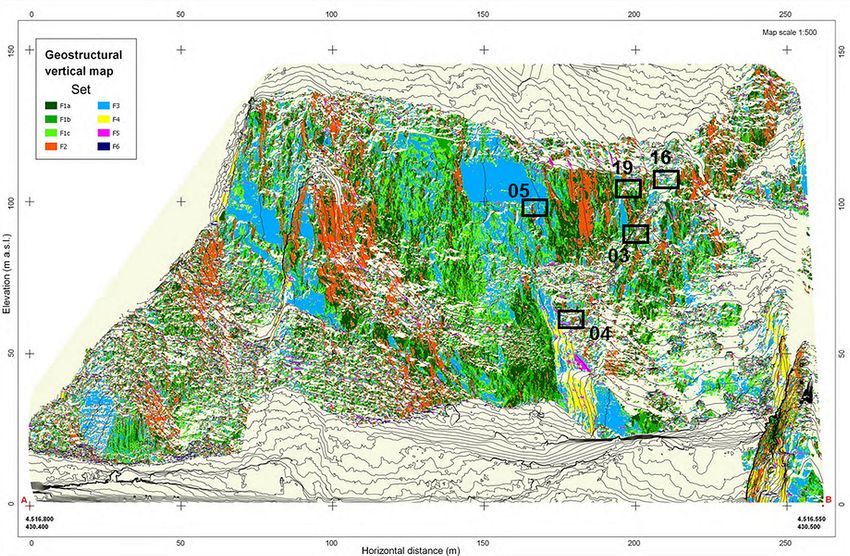
322                                                                            F. Matano et al.: Coroglio cliff integrated dataset

1   Introduction                                                    and to assess eventual relationships between meteorological
                                                                    factors (temperature, rain, wind, humidity, atmospheric pres-
Rocky coastal cliffs are located at the transition zone between     sure, etc.) and deformation of rocks. In addition, the statis-
subaerial and marine geomorphic systems. They represent a           tical analysis of multi-temporal datasets we present in this
very dynamic environment influenced by complex geologi-             study may provide an experimental basis for the appropriate
cal evolution on both regional and local scales (Emery and          definition of tuff failure early-warning system setup.
Kuhn, 1982; Bird, 2016; Sunamura, 1992). In fact, the evo-
lution of rocky coasts often occurs as a progressive retreat of
the cliff landward induced by a complex combination of ma-          2   Site description
rine (i.e., wave action) and subaerial processes (i.e., weath-
ering, erosion and mass wasting) (Sunamura, 2015). Future           The analyzed sector of the Coroglio cliff (Figs. 1b and 2) is
cliff recession could be more intense in the next decades un-       ∼ 140 m high and 250 m wide, with the aspect towards the
der the ongoing accelerating sea level rise thought likely to       SW. Different geological units and slope angles characterize
result from global warming (Bray and Hooke, 1997). In this          the cliff (Fig. 3). The upper part displays slope angles varying
context, sea cliff failures represent a serious hazard for popu-    from 35 to 45◦ and is formed by stiff to loose Holocene pyro-
lation living in coastal settlements. Severe retreat processes,     clastic deposits (LP unit) about 30 m in thickness, including
mainly occurring with landslides and erosion, are affecting,        a 2–3 m thick layer formed by very loose, reworked volcani-
for instance, many of the coastal cliffs forming the rocky          clastic deposits and soils at the top of the succession exposed
Italian coastline in various geological contexts (Iadanza et        on the cliff surface.
al., 2009; Furlani et al., 2014). Here, failures may affect cliff      The median part of the cliff is characterized by almost
formed by carbonate rocks (e.g., Andriani and Walsh, 2007;          vertical slope and is formed by two tuffaceous units, sep-
Ferlisi et al., 2012), arenaceous-pelitic or calcareous-pelitic     arated by an angular unconformity. The Neapolitan Yellow
flysch (e.g., Budetta et al., 2000; De Vita et al., 2012), sand-    Tuff (NYT) formation is a lithified ignimbrite deposit dated
stones (e.g., Sciarra et al., 2015), shales (e.g., Raso et al.,     at ∼ 15 ka (Deino et al., 2004). The NYT represents the up-
2017), or volcanic rocks (e.g., Barbano et al., 2014).              per unit in the outcrop and is formed by alternating coarse-
   The use of systems aimed at monitoring the slope stability       grained, matrix-supported breccia; thinly laminated lapilli
is becoming a standard practice to assess and prevent geo-          beds; and massive ash layers. The NYT displays a relatively
logical and geotechnical hazards and plan effective actions         homogeneous texture with several sub-planar surfaces likely
for hazard analysis and risk mitigation. Several on-site cliff      controlled by structural discontinuities and can be classi-
monitoring systems are operative in mountainous environ-            fied as weak to moderately weak rock (Froldi, 2000). The
ments (Pecoraro et al., 2018), as for example in the Swiss          Trentaremi (TTR) formation forms an older tuff cone dated
Alps (Spillmann et al., 2007), Bohemia (Zvelebill and Moser,        at ∼ 22.3 ka and represents the lower unit, consisting of
2001), Spain (Janeras et al., 2017) and Northern Apennines          slightly welded to welded, whitish to yellow, coarse-grained
(Salvini et al., 2015). These systems have the purpose of de-       pumiceous fragments embedded in a sandy ash matrix and
tecting and measuring small-scale rock deformations that can        lapilli beds. Diffused decimeter-scale vesicles and vacuoles
be regarded as precursors of slope failures. A more limited         due to differential erosion, markedly controlled by the bed-
number of monitoring systems is used for the analysis of            ding of the pyroclastic deposits, characterize the TTR rock
coastal cliffs and early-warning purposes (Clark et al., 1996;      face. These forms are typically related to the weathering due
Cloutier et al., 2015; Devoto et al., 2013). In our research        to salty seawater and wind erosion (Ietto et al., 2015).
(Matano et al., 2015, 2016; Esposito et al., 2017, 2018; Ca-           The tuff units cropping out at the Coroglio cliff are char-
puto et al., 2018), we focus on the in situ measurements            acterized by a complex system of mostly steep and pla-
of deformations affecting rocky blocks that form part of a          nar structural discontinuities and fractures (Matano et al.,
volcaniclastic coastal cliff located along the coastal sector       2016) showing highly variable spacing, well-developed NE–
of the Phlegraean Fields, a densely urbanized volcanic area         SW and NW–SE directions, and subordinate N–S and E–W
in southern Italy (Fig. 1a). In this area, marine coastal cliffs    trends. The base of the cliff is covered by slope talus breccia
are engraved in different volcanoclastic deposits (mainly tuff      (dt), partly occurring directly along the shoreline. These de-
and weakly welded ash and pumice layers), representing, in          posits are produced by the frequent failures occurring along
many cases, erosional relicts of volcanic edifices formed dur-      the cliff. The cliff instability is due to several causes, such as
ing explosive eruptions that occurred at Phlegraean Fields in       the complex volcano-tectonic evolution, the severe anthropic
the last 15 kyr. In detail, we present the database of measure-     modifications (i.e., excavations, tunneling and so on) of the
ments obtained by an integrated monitoring system imple-            coastline since Roman times and weathering and erosion pro-
mented at the Coroglio coastal tuff cliff, located in the highly    cesses occurring at the boundary between coastal and marine
urbanized coastal area of Naples (Italy) (Fig. 1a). The main        environments. The last relevant tuff failures occurred around
aims of the research are to identify range and patterns of de-      1990 (Froldi, 2000) along the southern sector of the cliff
formation during a potential pre-failure stage of rock blocks       (Fig. 2). Due to the severe instability conditions, the upper

Earth Syst. Sci. Data, 12, 321–344, 2020                                              www.earth-syst-sci-data.net/12/321/2020/
F. Matano et al.: Coroglio cliff integrated dataset 323
Figure 1. (a) Study area location and Phlegraean Fields area. (b) Detailed study area orthophoto (2004). The hillshade (a) and the orthophoto
(b) in the background are from the year 2004 (courtesy of Regione Campania). Hillshade derives from a 5 m pixel DTM of the Carta Tecnica
della Regione Campania (CTR) topographic map at 1 : 5000 scale, with 447 153 and 465 034 sheets (https://sit2.regione.campania.it/content/
carta-tecnica-regionale-2004-2005; last access: 5 January 2020). The orthophoto is a mosaic of 447 153 and 465 034 orthophoto maps at the
1 : 5000 scale (https://sit2.regione.campania.it/content/ortofoto-campania-20042005; last access: 5 January 2020).
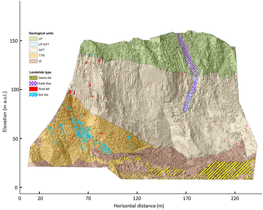
for obtaining a detailed multi-temporal digital terrain model
(DTM) of the cliff (Caputo et al., 2018) that allowed map-
ping of the landslides that occurred during the period be-
tween 29 April 2013 and 4 March 2015 (Fig. 3). In detail,
four types of landslides (rock fall, debris fall, earth flow and
soil slip) have been recognized in the different sectors of the
cliff (Fig. 3). These have caused a total eroded/fallen volume
of about 3500 m3 of volcanic material (rock and soil), and
the related short-term retreat rate of the entire cliff has been
assessed at about 0.07 m yr−1 during 2013–2015 (Caputo et
Figure 2. Coroglio cliff view from the WSW. The red dashed line al., 2018). Based on a geomorphological analysis, including
shows the area mapped in Fig. 3, the yellow dotted line shows the cliff inspections carried out by climber geologists and inter-
area involved by reinforcement works, the light blue circle shows pretation of the multi-temporal DTMs, an area with several
the area with unstable tuff blocks and the red arrow shows the de-
unstable tuff blocks (Fig. 2) has been recognized in the NYT
tachment area of the failure that occurred around 1990, located out-
side the area mapped in Fig. 3. Black lines separate the upper, me-
unit sector of the cliff (Fig. 3). This area has been selected
dian and lower parts of the cliff. for implementing the monitoring system.
3 Data and methods
part of the northern sector of the tuff cliff was subject to rein-
3.1 The monitoring system
forcement works (Fig. 2) at the beginning of the 2000s. These
consisted in a wire mesh and steel cable network applied to Based on the results of the geostructural and geomorpholog-
the tuff wall steel reinforced with bars anchored and bolted ical surveys, a series of prismatic tuff blocks, bounded by
to the rock. open fractures, have been selected for the instrumental mon-
During the first phase of the research, we have integrated itoring (Figs. 4 and 5). The accurate detection of structural
the results of long-range terrestrial laser scanner (TLS) discontinuities and morphometric parameters of the selected
surveys with structural field mapping to obtain a detailed tuff blocks resulted in the understanding of the possible fail-
geostructural analysis and classification of the slope (Fig. 4) ure mechanism and their kinematic analysis. Volumes of the
(Matano et al., 2016). Repeated TLS surveys have been used selected tuff blocks range between 4 and 15 m3 , and the pos-
www.earth-syst-sci-data.net/12/321/2020/ Earth Syst. Sci. Data, 12, 321–344, 2020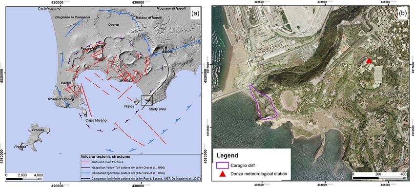
324                                                                                 F. Matano et al.: Coroglio cliff integrated dataset

Figure 3. Geological vertical map of the Coroglio cliff (modified after Matano et al., 2016). Landslide types that occurred during the 2013–
2015 interval (Caputo et al., 2018) are also shown. Geological units: LP, stiff to loose recent pyroclastic deposits and soils; LP-NYT, thin
layer of LP deposits on NYT unit; NYT, Neapolitan Yellow Tuff; TTR, Trentaremi Tuff; dt, slope talus breccia and gravelly beach deposits.

sible failure kinematics are toppling, planar and wedge slid-              The DeMSys is formed by a meteorological
ing (Table 1).                                                          station (DAVIS, model Vantage Pro2 – wireless;
   The installed monitoring system consists of both standard            see      at:      https://www.davisinstruments.com/support/
geotechnical instruments, such as crackmeters and tiltmeters            vantage-pro2-wireless-stations/, last access: 5 Jan-
equipped with a near-rock-surface thermometer, installed in             uary 2020), located less than 1 km away from the cliff
correspondence with the five selected unstable tuff blocks,             (Fig. 1b), characterized by a wireless Integrated Sensor
and a weather station equipped with a thermometer, barom-               Suite (ISS) including barometer, hygrometer, pluviometer
eter, hygrometer, anemometer and rain gage sensors. The                 and thermometer integrated sensors and an anemometer
used instrumentation forms two separate linked sub-systems:             (Table 3). The CC-MoSys tuff monitoring unit records 16
the Coroglio cliff Monitoring System (CC-MoSys) and the                 parameters (Table 4) with a frequency set to 30 min for
Denza Meteorological Station (DeMS) (Fig. 1b).                          48 daily measures. The weather station unit records nine
   Specifically, the CC-MoSys is formed by nine monax-                  parameters (Table 5) with a frequency of measurements set
ial electric crackmeters (model BOVIAR BTS LWG 100),                    up 10 min for 144 daily measures. Continuous data recording
one external thermistor (model BOVIAR NTC/A 10K)                        of geotechnical sensors was active from December 2014 to
and two biaxial tiltmeters (model BOVIAR BIAX-B/T)                      October 2018, whereas the weather station has been active
equipped with internal thermistors (model BOVIAR NTC/A                  since January 2014. The meteorological time series analyzed
10K) (Table 2). The geotechnical sensors have been in-                  in this work are updated to December 2018. The monitoring
stalled across or on the face of the fractures bounding                 system has been regularly controlled and maintained so as
the five unstable tuff blocks in order to provide an accu-              to ensure full accuracy in measures, even if some missing
rate monitoring of displacements and rotations. Each sen-               data intervals are present due to the occurrence of some
sor is individually cabled to the acquisition unit (model               functional interruptions of the acquisition units.
BOVIAR eDAS 16ch; see at: https://www.boviar.com/it/                       Overall, the monitored parameters include both deforma-
prodotti/centralina-di-acquisizione-dati-edas-2/, last access:          tion and meteorological ones:
5 January 2020), located at the top of the cliff.

Earth Syst. Sci. Data, 12, 321–344, 2020                                                   www.earth-syst-sci-data.net/12/321/2020/
F. Matano et al.: Coroglio cliff integrated dataset 325
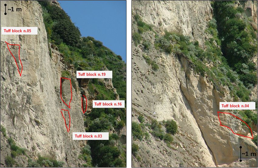
Figure 4. Geostructural vertical map (modified by Matano et al., 2016). Black boxes show location of the monitored unstable tuff blocks.
Set legend (dip–dip direction): F1a (> 65◦ /30–50◦ and 220–235◦ ), F1b (> 65◦ /50–60◦ and 235–245◦ ), F1c (> 65◦ /55–65◦ and 245–255◦ ),
F2 (> 65◦ /0–30◦ and 180–220◦ ), F3 (> 70◦ /60–110◦ and 255–280◦ ), F4 (> 70◦ /110–180◦ and 300–355◦ ), F5 (20–65◦ /50–195◦ ) and F6
(< 20◦ /0–360◦ ).
Table 1. Geostructural characteristics of the monitored tuff blocks.
No. Size (width, length, Cliff local Joint sets∗ Kinematic ID ID
height; volume) orientation∗ crackmeter tiltmeter
3 4.0, 2.0, 1.5 m; 12.0 m3 85◦ /235◦ 82◦ /100◦ , 80◦ /5◦ , 85◦ /90◦ wedge sliding, toppling 03F1 –
4 1.5, 5.0, 1.0 m; 7.5 m3 88◦ /255◦ 35◦ /240◦ , 85◦ /20◦ , 15◦ /290◦ planar sliding 04F1 04I1
5 2.0, 2.0, 1.5 m; 6.0 m3 85◦ /275◦ 80◦ /100◦ , 75◦ /20◦ , 75◦ /230◦ wedge sliding, toppling 05F1, 05F2, 05F3 –
16 2.0, 2.0, 1.0 m; 4.0 m3 80◦ /330◦ 70◦ /5◦ , 80◦ /350◦ , 78◦ /205◦ wedge sliding 16F1, 16F2 –
19 5.0, 2.0, 1.5 m; 15.0 m3 87◦ /250◦ 88◦ /60◦ , 85◦ /240◦ , 48◦ /5◦ toppling 19F1, 19F2 19I1
∗ Orientation is expressed with dip and dip direction values in the format “dip/dip direction”.
– variation in the cracks’ opening and displacement (slid- The data acquisition and broadcasting system is fully re-
ing) along tuff cracks, motely controlled. Rechargeable batteries and a solar panel
provide the power supply for the monitoring system. Twice a
– slope angle variations (rotation) in tuff block surfaces, day, the measured data are transferred via a GSM (Global
System for Mobile Communications) network to a master
– air temperature and near-rock-surface air temperature, station located in the ISMAR (Istituto di Scienze Marine)
research institute, where data are directly stored in a dedi-
– humidity,
cated NAS (network-attached storage) system and converted
– wind (velocity and direction), to open-access files for our data repository.
– barometric pressure,
– rainfall (rain quantity and rate).
www.earth-syst-sci-data.net/12/321/2020/ Earth Syst. Sci. Data, 12, 321–344, 2020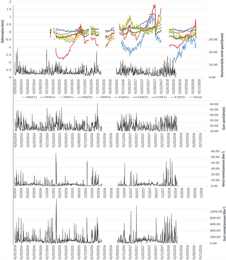
326                                                                                    F. Matano et al.: Coroglio cliff integrated dataset

Table 2. Technical specifications of the sensors in CC-MoSys cabled with the acquisition unit – model eDAS 16ch.

                                                                                                                      Update
                   Sensor          Parameter       Sensitivity   Operational range        Accuracy                    interval
                   Crackmeter      displacement    0.01 mm       −50.0 to 50.0 mm         ±0.05 % (−30 to 100 ◦ C)    30 min
                   Tiltmeter       angle           0.01◦         −10.0 to 10.0◦           ±1 % (−20 to 80 ◦ C)        30 min
                   Thermistor      temperature     0.1 ◦ C       −30.0 to 70 ◦ C          ±2.5 ◦ C (−20 to 70 ◦ C)    30 min

Table 3. Technical specifications of the sensors of the used meteorological station – model DAVIS Vantage Pro2 wireless in DeMS.

                                                             Data resolution                                     Sampling
                     Sensor           Parameter              and unit             Range              Accuracy    rate
                     Anemometer       wind speed             0.5 m s−1            0–89 m s−1         ±1 m s−1    3s
                                                             (or 0.97 kn)                            or 5 %
                     Anemometer       wind direction         1◦                   0–360◦             ±3◦         3s
                     Barometer        barometric pressure    0.1 hPa              540–1100 hPa       ±1 hPa      1 min
                     Hygrometer       relative humidity      1%                   1 %–100 %          ±2 %        1 min
                     Rain gauge       rainfall amount        0.25 mm              0–999.8 mm         ±4 %        20–24 s
                     Rain gauge       rainfall rate          0.1 mm h−1           0–2438 mm h−1      ±5 %        20–24 s
                     Thermometer      air temperature        0.1 ◦ C              −40 to 65 ◦ C      ±0.3◦ C     10–12 s

                                                                            measurements acquired for 1404 d (from 3 December 2014
                                                                            to 6 October 2018). Some missing data intervals are present
                                                                            due to the occurrence of some functional interruptions of the
                                                                            eDAS acquisition unit; for two sensors (F04F1 and F16F2),
                                                                            missing data intervals are larger (Table 6) due to the occur-
                                                                            rence of mass movements on the cliff that damaged the two
                                                                            sensors.
                                                                               We compute some descriptive statistics for summariz-
                                                                            ing the different features of the deformation measurement
                                                                            dataset (Table 6). These statistics are the results of a univari-
                                                                            ate analysis, describing the distribution of each single vari-
                                                                            able, including its central tendency (mean and median) and
                                                                            data dispersion (including minimum and maximum values,
                                                                            quartiles, and standard deviation).
Figure 5. Unstable tuff blocks of the NYT unit selected for moni-
toring activity (red lines).
                                                                            3.3   Meteorological data

3.2   Tuff deformation data
                                                                            The database of DeMS measurements (Fortelli et al., 2019)
                                                                            encompasses 262 944 measurements acquired with a 10 min
The deformation data consist of measurements of displace-                   interval for 1826 d spanning from January 2014 to Decem-
ment across the fractures bounding tuff blocks along the di-                ber 2018.
rection of the crackmeters’ axis and of both horizontal and                    Some missing data intervals are present due to the occur-
vertical angles associated with rotation of the rock blocks                 rence of some functional interruptions of the DAVIS acqui-
(Table 2). The instruments have collected measurements ev-                  sition unit; the missing data intervals are larger only for the
ery 30 min for a period of about 4 years. These measurements                anemometric sensor data (i.e., Wi_speed and HiWi_spe) due
are expressed for each sensor as relative measurements with                 to a technical issue of the sensor during 2018. The descriptive
respect to the initial measurement, considered to be a ref-                 statistics resulting from a univariate analysis of the acquired
erence zero value. We also measured near-rock-surface air                   dataset, with the exception of wind and gust direction, are
temperature (as a proxy for surface rock temperature) us-                   shown in Table 7.
ing some thermistors installed at three locations on the cliff                 We added to the database two numeric parameters that
(i.e., near the acquisition unit and near the tiltmeter boxes).             take into account the direction of wind and gust, i.e., wind
In this way, the CC-MoSys database encompasses 67 355                       pressure (Wi-P_norm) and gust pressure (HiWi-P_norm), ex-

Earth Syst. Sci. Data, 12, 321–344, 2020                                                       www.earth-syst-sci-data.net/12/321/2020/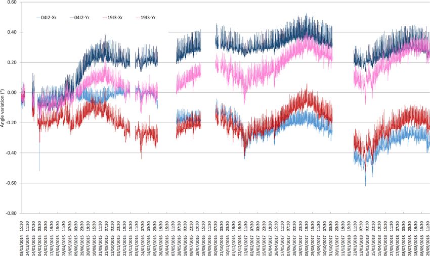
F. Matano et al.: Coroglio cliff integrated dataset                                                                                                  327

Figure 6. Data distribution of measurements of crackmeters (03F1, 04F1, 05F1, 05F2, 05F3, 16F1, 16F2, 19F1 and 19F2).

Table 4. List of measured tuff deformation parameters in CC-MoSys.

  Parameter   Short    Parameter                             Tuff
  code        name     name           Unit    Sensor type   block   Description of measured parameter
  03F1        DIS      displacement   (mm)    crackmeter      03    displacement measured across crack F1 bounding tuff block no. 03 during last 30 min
  04F1        DIS      displacement   (mm)    crackmeter      04    displacement measured across crack F1 bounding tuff block no. 04 during last 30 min
  05F1        DIS      displacement   (mm)    crackmeter      05    displacement measured across crack F1 bounding tuff block no. 05 during last 30 min
  05F2        DIS      displacement   (mm)    crackmeter      05    displacement measured across crack F2 bounding tuff block no. 05 during last 30 min
  05F3        DIS      displacement   (mm)    crackmeter      05    displacement measured across crack F3 bounding tuff block no. 05 during last 30 min
  16F1        DIS      displacement   (mm)    crackmeter      16    displacement measured across crack F1 bounding tuff block no. 16 during last 30 min
  16F2        DIS      displacement   (mm)    crackmeter      16    displacement measured across crack F2 bounding tuff block no. 16 during last 30 min
  19F1        DIS      displacement   (mm)    crackmeter      19    displacement measured across crack F1 bounding tuff block no. 19 during last 30 min
  19F2        DIS      displacement   (mm)    crackmeter      19    displacement measured across crack F2 bounding tuff block no. 19 during last 30 min
  04I2-X      Angle    angle          (◦ )    tiltmeter       04    variation in horizontal angle measured in tuff block no. 04 during last 30 min
  04I2-Y      Angle    angle          (◦ )    tiltmeter       04    variation in vertical angle measured in tuff block no. 04 during last 30 min
  04I2-T      T tech   temperature    (◦ C)   thermistor      04    external temperature close to sensor I2 (average in 30 min)
  19I3-X      Angle    angle          (◦ )    tiltmeter       19    variation in horizontal angle measured in tuff block no. 19 during last 30 min
  19I3-Y      Angle    angle          (◦ )    tiltmeter       19    variation in vertical angle measured in tuff block no. 19 during last 30 min
  19I3-T      T tech   temperature    (◦ C)   thermistor      19    external temperature close to sensor 19 (average in 30 min)
  Temp-1      TTT      temperature    (◦ C)   thermistor       –    external air temperature near acquisition unit (average in 30 min)

pressed in newtons per square meter. They are for the normal                 where Pn is wind/gust pressure normal to the cliff expressed
component of the pressure exerted by the wind/gust on the                    in newtons per square meter, veln is wind velocity normal
rock face on the cliff. We calculated the normal component                   to the cliff expressed in meters per second, and 0.613 is the
of the wind velocity by considering the angle between cliff                  coefficient based on average values of air density and grav-
average aspect orientation, that is towards the WSW (i.e.,                   itational acceleration expressed in reciprocal kilograms per
247.5◦ ), and the wind/gust direction. Winds blowing from                    meter.
the direction of 337.5 to 360◦ and from 0 to 157.5◦ do not
produce pressure on the rock surface, as they are sheltered                  4     Results
from the cliff itself. Winds blowing from directions between
157.5 and 337.5◦ produce a normal component of pressure                      4.1    Deformation trends
that varies under the cosine of the incidence angle with the
cliff (ranging from 0 to 90◦ ). Once we have calculated the                  Crackmeter data usually show value ranges between 0.48 and
vertical component of the wind/gust, we may calculate the                    1.98 mm, with the two relevant exceptions of 04F1 and 05F2
wind/gust pressure normal to the cliff with the simplified for-              with ranges of 5.56 and 4.31 mm, respectively. Tiltmeter data
mula (ASCE, 2013)                                                            show a lower variability as value intervals range between
                                                                             0.38 and 0.78◦ (Table 6). In more detail, the data distribu-
                                                                             tion analysis shows some different trends for the data of the
                                                                             different sensors (Fig. 6). Data of the 03F1 sensor show an
Pn = 0.613 veln2 ,                                                  (1)      asymmetric distribution with a modal value around −1 mm

www.earth-syst-sci-data.net/12/321/2020/                                                           Earth Syst. Sci. Data, 12, 321–344, 2020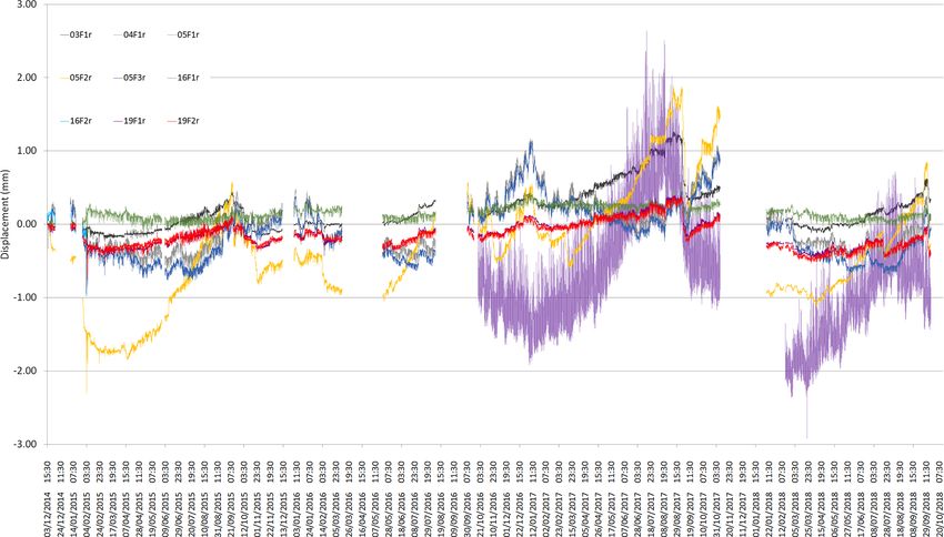
328                                                                                              F. Matano et al.: Coroglio cliff integrated dataset

Table 5. List of measured meteorological parameters in DeMSys.

  Parameter
  code           Short name           Parameter name           Unit           Sensor type       Description of measured parameter
  Temp           TTT                  air temperature          (◦ C)          thermometer       air temperature (average in 10 min)
  Hum            RH                   relative humidity        (%)            hygrometer        relative humidity (average in 10 min)
  Wi-spe         ff                   wind speed               (m s−1 )       anemometer        wind speed (average in last 10 min)
  Hi-Wi-spe      ff gust              gust speed               (m s−1 )       anemometer        maximum gust speed during last 10 min
  Wi-dir         Wind dir descr       wind direction           (◦ )           anemometer        prevalent direction of wind during last 10 min
  Hi-Wi-dir      Wind dir descr       gust direction           (◦ )           anemometer        direction of maximum gust during last 10 min
  Bar            PPPP                 barometric pressure      (hPa)          barometer         site atmospheric pressure (average in 10 min)
                                                                                                adjusted to sea level atmospheric pressure
  Rain           Precip               rainfall amount          (mm)           pluviometer       rainfall amount (cumulated on 10 min)
  Rain rate      Precip               rainfall rate            (mm h−1 )      pluviometer       maximum instantaneous rainfall rate during last 10 min

Table 6. Descriptive statistics of tuff deformation data and temperatures measured by CC-MoSys.

                                                                                            Third                      Standard        No. of
                                  Minimum    First quartile     Median         Mean       quartile     Maximum         deviation     measures
                F03F1               −0.53            −0.01        0.13        0.201          0.34               1          0.302         53618
                F04F1               −2.92            −1.21       −0.79        −0.68         −0.27            2.64          0.783         29551
                F05F1               −0.85            −0.29       −0.04       −0.001          0.22               1          0.345         55058
                F05F2               −2.31            −0.84       −0.32       −0.316          0.13               2          0.758         55058
                F05F3               −0.98            −0.44        −0.1       −0.112          0.14               1          0.382         55058
                F16F1               −0.29             0.09        0.15         0.16          0.24            0.43          0.091         55058
                F16F2               −0.28            −0.08           0         0.02          0.13             0.2          0.113          1339
                F19F1               −0.79            −0.29       −0.17       −0.142         −0.02            0.39          0.182         55058
                F19F2               −0.84            −0.28       −0.17       −0.151         −0.04            0.39          0.177         55058
                F04I2-X             −0.62            −0.28       −0.19       −0.179         −0.04            0.08          0.137         55058
                F04I2-Y             −0.26              0.2        0.27        0.234          0.31            0.53          0.129         55058
                F19I3-X             −0.53            −0.25        −0.2       −0.205         −0.15            0.06          0.082         55058
                F19I3-Y             −0.33             0.03         0.1        0.112          0.21            0.41          0.119         55058
                F04I2-T             −0.01            13.65       19.04        19.18         24.23           42.79          6.844         55058
                F19I3-T             −1.36             12.5       17.72        17.84         22.93           38.58          6.584         55058
                Temp-1               0.86             13.6        18.6        18.54          23.5           43.86          6.012         55058
                Temp∗                −2.8             12.6        16.5        17.27         22.27           34.20          5.877         79473
              ∗ Temp data, measured by DeMSys from 1 January 2013 to 31 December 2018, have been aggregated to 30 min for comparison with CC-MoSys
              temperature data.

and higher coda values up to 3 mm. The 04F1 data show a                            similarity in recorded values suggests a uniform behavior of
uniform distribution between −0.1 and 3 mm. Parameters of                          the lateral crack.
block 05 have a very large range of variability, with a well-                         The tiltmeter data have been reported in Fig. 8 for 04I2
defined main value only for F2 sensor. F1 and F3 sensors                           and 19I3 sensors. The X (horizontal) components recorded
show a very high correlation (Fig. 7), suggesting a uniform                        prevalently negative variation, while the Y (vertical) com-
behavior of the crack in the section covered by them. All                          ponents were positive over the entire time interval of the
three sensors recorded large distribution of both positive and                     datasets. This evidence shows how the rock block moves and
negative values, indicating a strong dynamic behavior. On                          turns during the time to some preferred position (the higher
the other hand, the 16F1 sensor (Fig. 6) shows a mono-modal                        histogram bar). For the 19I3 sensor, a small range of vari-
distribution well centered around 0.2 mm (with an oscillation                      ability has been observed, about 0.4◦ , and a tiny distribution
of ±0.1 mm). The stability of the values across time could                         around 0.3–0.4◦ for the Y component. A similar behavior is
highlight a stable dynamic position reached from the block.                        shown by component X where the equilibrium position is
The 16F2 sensor worked for a very short time compared with                         characterized by angle values between −0.2 and −0.3◦ .
the others. However, the data distribution shows two main                             The temperature value distribution of the three thermistors
values of 0.0 and 0.2 mm. The F1 and F2 sensors, located on                        appears coherent and well centered in a range between +13
tuff block 19, show a quite identical behavior (Fig. 6). The                       and +25 ◦ C (Fig. 9). If we compared those temperature data

Earth Syst. Sci. Data, 12, 321–344, 2020                                                                 www.earth-syst-sci-data.net/12/321/2020/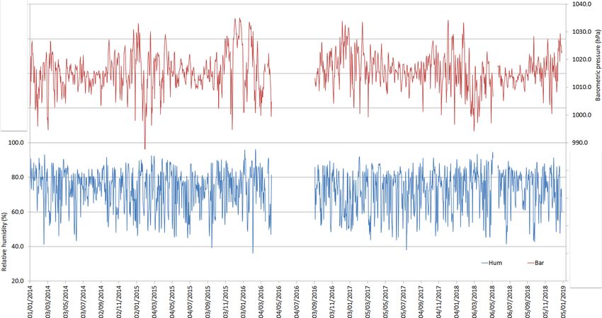
F. Matano et al.: Coroglio cliff integrated dataset                                                                            329

Table 7. Descriptive statistics of temperature and meteorological data measures by DeMS.

                                            First                          Third                  Standard      No. of
                             Minimum      quartile   Median      Mean    quartile    Maximum      deviation   measures
                Temp             −2.9        12.6       16.5     17.2         22.1       33.8          5.8     238 422
                Hum               23.0       64.0       75.0     72.8         83.0       98.0         13.4     238 418
                Bar              982.7     1011.9     1015.6   1015.8       1019.7     1036.8          6.9     238 793
                Rain               0.0        0.0        0.0      0.0          0.0       17.6          0.2     238 500
                Rain rate          0.0        0.0        0.0      0.3          0.0      292.6          4.3     238 500
                Wi_speed           0.0        1.7        3.5      4.4          6.1       40.9          3.5     200 945
                HiWi_spe           0.0        4.3        7.8      8.7         11.3       61.7          6.0     200 945

Figure 7. Correlation plot between 05F1 and 05F3 data.

with air temperature measurements provided by the weather             meters show from +0.1 to +1.2 mm cumulative deformation
station installed in the vicinity (Fig. 10), time series show,        (Fig. 11), while tiltmeters show from 0.1 to 0.4◦ cumulative
as usual for this climatic region, clear seasonal variation pat-      angle variation (Fig. 12).
terns and annual cyclicity with some small differences. In de-
tail, near-rock-surface air temperatures show minimum val-            4.2    Thermal trends
ues from 2.8 to 3.7 ◦ C higher and maximum values from 4.4
to 9.7 ◦ C higher than air temperatures (Table 6). Amplified          Temperature time series data (Fig. 10) show a clear seasonal
near-rock-surface air temperatures could result in consequent         cyclicity and inter-annual variation patterns. Air temperature
increases in crack deformation forces.                                values range between −2.9 and 33.8 ◦ C throughout the 5
   If we consider the time distribution of measured data, both        years of measurements.
crackmeters and tiltmeters show several evidence of tuff de-             Average temperature values of the 5-year period have been
formation through time. The time series of the measured               plotted for the average daily value analysis, daily minimum
crack aperture and plane rotation data reveal a deformation           temperature (Tmin ) and daily maximum temperature (Tmax )
pattern characterized by both diurnal and seasonal cyclical           in order to observe the annual trends and detect the most
deformation (Figs. 11 and 12). The data plots for a single            significant surplus or deficit thermal phases (Fig. 14). Dia-
year of measurements show a similar repetitive pattern with           grams also report interpolation curves relative to minimum
lower values in late winter and higher values in late sum-            and maximum daily values (fourth-grade polynomial equa-
mer (Fig. 13), showing significant correlation with seasonal          tion); we also computed the difference between the minimum
temperature trends. Some trends of cumulative multi-annual            and maximum temperatures (1T ).
changes, based on about 4 consecutive years of data (Decem-              In detail, we have evaluated the thermal increase between
ber 2014 to October 2018), can also be recognized. Crack-             the late winter minimum and summer maximum and the au-
                                                                      tumn thermal decrease between the summer maximum and

www.earth-syst-sci-data.net/12/321/2020/                                                   Earth Syst. Sci. Data, 12, 321–344, 2020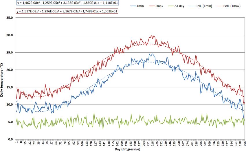
330                                                                              F. Matano et al.: Coroglio cliff integrated dataset

Figure 8. Data distribution of measurements of tiltmeters (04I2-X, 04I2-Y, 19I3-X and 19I3-Y).

Figure 9. Data distribution of measurements of thermistors (19I3-T, 04I2-T and Temp-1).

late December minimum. From the analysis of fourth-grade                    Spring thermal increase is
polynomial equations of annual thermal trend, relative to                   1T + (min) = Tmin (max) – Tmin (1) (min) = 13.9 ◦ C,
daily Tmin and Tmax , the following values have been derived:
                                                                            1T + (max) = Tmax (max) – Tmax (1) (min) = 15.2 ◦ C.
      Tmin (1) (min) = 8.0 ◦ C (05/02)
      Tmax (1) (min) = 12.3 ◦ C (04/02)                                     Autumn thermal decrease is
                                                                            1T − (min) = Tmin (max) – Tmin (2) (min) = 14.0 ◦ C,
      Tmin (max) = 21.9 ◦ C (30/07)                                         1T − (max) = Tmax (max) – Tmax (2) (min) = 15.3 ◦ C.
      Tmax (max) = 27.5 ◦ C (02/08)
                                                                      The main features highlighted by the analysis are the follow-
      Tmin (2) (min) = 7.9 ◦ C (31/12)                                ing:
      Tmax (2) (min) = 12.2◦ C (31/12).
                                                                         – an annual trend showing a wave characterized by a weak
Thermal yearly excursions are therefore equal as follows.                  thermal excursion, for both minimum and maximum

Earth Syst. Sci. Data, 12, 321–344, 2020                                                  www.earth-syst-sci-data.net/12/321/2020/
F. Matano et al.: Coroglio cliff integrated dataset 331
Figure 10. Temperature time series showing daily, seasonal and annual variation patterns. Long-term trends, based on about 5 consecutive
years of data, show annual cyclicity. Air temperature and near-rock-surface air temperature are fully synchronous; peaks in near-rock-surface
air temperatures (19I3-T, 04I2-T and Temp-1) are sometimes higher than those of air temperature (Temp). Data are incomplete in some
months.
Figure 11. Crack aperture variation time series showing daily, seasonal and annual deformation patterns. Long-term trends, based on about
4 consecutive years of data (December 2014 to October 2018), show from +0.1 to +1.2 mm of cumulative deformation. Data are incomplete
in some months.
daily values, probably associated with the proximity to – an extremely mild winter season, with only a few days
the sea; with minimum temperatures below 5 ◦ C;
– a summer season with only a few days with daily maxi-
mum temperature above the threshold value of 30 ◦ C; – a weak daily thermal excursion, with values of gener-
ally ∼ 5 ◦ C and only a few days with a daily thermal
excursion > 10 ◦ C.
www.earth-syst-sci-data.net/12/321/2020/ Earth Syst. Sci. Data, 12, 321–344, 2020332 F. Matano et al.: Coroglio cliff integrated dataset Figure 12. Angle variation time series data showing daily, seasonal and annual deformation patterns. Long-term trends, based on about 4 consecutive years of data (December 2014 to October 2018), show from 0.1 to 0.4◦ of cumulative angle variation. Horizontal and vertical angle variation shows opposite evidence for each block. Data are incomplete in some months. Figure 13. Annual time series plots of the 05F2 crackmeter showing partly repetitive seasonal deformation patterns. In detail, the annual thermal trend in the analyzed period is winter there were not any long periods characterized by sig- characterized by 3 years (2016–2018) with values close to nificantly low temperatures, with the two exceptions of the the average values of the investigated period and 2 years with period between 5 and 15 January 2017 (with values close significant differences during the summer season. In detail, to zero and a minimum of −1.6 ◦ C) that also caused weak summer 2014 had values significantly lower than the average snowfalls, and a very cold and snowy phase at the end of values, and summer 2015 had values characterized by a clear February 2018. thermal surplus during the months of July and August, when the threshold value of 30 ◦ C was exceeded on 22 d. During Earth Syst. Sci. Data, 12, 321–344, 2020 www.earth-syst-sci-data.net/12/321/2020/
F. Matano et al.: Coroglio cliff integrated dataset                                                                              333

Figure 14. Average daily thermal trend, for 2014–2018, recorded by Denza weather station with fourth-grade polynomial equations. Maxi-
mum temperature values are indicated with a red line, minimum values with a blue line and daily temperature range with a green line.

4.3   Rainfall trends                                                vs. 181.4 mm), autumn (281.9 mm vs. 317.6 mm) and winter
                                                                     (259.4 mm vs. 290.9 mm) rainfall amounts are slightly below
Rain and rain rate data time series are plotted in Fig. 15.          the MOUF climatologic reference. The winter precipitation
Rainfall is characterized by a considerable irregularity, with       deficit is due to a strong negative rain anomaly observed at
sometimes extremely high accumulation values and rates               Denza during December 2015 (0.3 mm) and 2016 (9.5 mm).
(October 2015, September 2017) usually associated with late          During 2015, a rainfall regime with a large prevalence of dry
summer storms, alternating with periods of modest rainfall           months was compensated for by 3 very rainy months, Jan-
even in seasonal phases in which rainfall is generally abun-         uary, February and October, the last one characterized by a
dant (December 2015 and 2016). Rainfall (measured at in-             rainfall amount of 195.5 mm. The year 2017 has been charac-
tervals of 10 min) reached a maximum value of 17.6 mm                terized by a severe rainfall deficit with a total annual precipi-
on 12 September 2014, corresponding to a rain rate of                tation amount of 536.8 mm; in particular, summer 2017 rain-
105.6 mm h−1 . The maximum rain rate of 292.6 mm h−1 was             fall was only 4.1 mm, suggesting extremely dry conditions
recorded on 19 September 2016.                                       for this season. Instead, the year 2018 has been characterized
   We plotted the average values for the whole 5-year pe-            by a total annual rainfall amount of 902.1 mm, slightly above
riod of the monthly total rainfall amounts (Fig. 16). In or-         MOUF climatologic values.
der to evaluate the occurrence of rainfall surplus or deficit
periods, these values are compared with the monthly aver-            4.4   Wind trends
age values of rainfall, for the 1872–2005 time period, mea-
sured at the Meteorological Observatory (MOUF) of the                Wind and gust speed data time series are plotted in Fig. 17.
University of Napoli “Federico II” (Mazzarella, 2006). It            Wind velocity and gust velocity (both measured at 10 min in-
is worth noting that the monthly precipitation average val-          tervals) reached the maximum values of 40.9 kn (11.8 m s−1 )
ues over the analyzed 5-year period (2014–2018) tend to              and 61.7 kn (31.7 m s−1 ), respectively (Table 7).
converge towards those values of climatological relevance               The wind regime indicates considerable consistency, both
recorded in Naples at MOUF (Mazzarella, 2006), thus re-              in terms of anemoscopic regime (wind provenance direction)
flecting the strong pluviometric characterization of the site.       and in terms of average intensity. The seasonal regimes are
Data analysis highlights some peculiarities in the rainfall          characterized by the repetition of the anemometric patterns,
conditions that affect the area. The average annual rain-            highlighting the occurrence of local structural factors that,
fall amount of 759.6 mm is below the amount of the cli-              even if in interaction with the meteorological conditions on a
matological reference of 866.0 mm. In detail, the summer             synoptic (cyclonic) scale, are able to control the wind regime
rainfall amount is almost equal to the MOUF climatologic             in the considered coastal sector. Tables 8 and 9 summarize
reference (69.0 mm vs. 75,7 mm), while spring (149.3 mm              the annual and monthly average values of average wind speed

www.earth-syst-sci-data.net/12/321/2020/                                                Earth Syst. Sci. Data, 12, 321–344, 2020
334 F. Matano et al.: Coroglio cliff integrated dataset
Figure 15. Rain amount (10 min) and rain rate time series data showing daily, seasonal and annual variation patterns in the Denza station
during 2014–2018.
fourth quadrants of the rose diagram, with the SE direction
reaching the maximum percentage weight. The direction as-
sociated with the maximum average wind speed values is the
SE–SSE directions. Therefore, we may infer that the spring
season is characterized by the alternation of south-eastern
and north-western winds, which are also associated with the
greatest average intensities. The polar diagram shows that
summer winds blow with a prevalence from the third and
fourth quadrants, with the WSW direction reaching the max-
imum percentage weight. The directions associated with the
maximum average wind speeds are the westerly ones. It is
therefore possible to state that the summer season is domi-
Figure 16. Average cumulative monthly rainfall data histogram for nated by breeze regime winds, typical of the coastal Mediter-
2014–2018. Diagram also reports average monthly values of rain-
ranean areas. However, it is worth underlining that the occur-
fall, measured at the Meteorological Observatory of University of
rence of SSE relatively high average intensities is not infre-
Naples “Federico II” since 1872 (Mazzarella, 2006). Rainfall val-
ues are reported in blue square cells and red square cells. quent. In the autumn season winds blow in a well-distributed
pattern in all sectors, with the SE–SSE direction reaching the
maximum percentage weight; also, the directions associated
Table 8. Annual average values of wind measures during 2014– with the maximum average wind speeds are the SE and SSE.
2018. It is therefore possible to state that the autumn season is nor-
mally dominated by Scirocco-like anemometric events, with
2014 2015 2016 2017 2018
associated very rough sea. During the winter season, the po-
Avg. wind speed 2.3 2.2 2.5 2.1 2.3 lar diagram highlights an anemoscopic regime very similar
Dominant direction SSE SSE SSE SSE SSE to the autumn one. In fact, it may be observed that the synop-
Maximum gust 23.7 27.8 31.8 22.8 28.2 tic winds blow in a well-distributed way involving quadrants
one, two and four, with the SE and NE directions reaching the
maximum percentage weight. The provenance directions as-
(m s−1 ), dominant direction of the wind (sector of 22.5◦ ) and sociated with the maximum average wind speeds are namely
maximum wind gust (m s−1 ). Wind average speed can usu- SE and SSE.
ally be categorized as level 2 on the Beaufort scale, while By considering the angle between wind/gust direction and
gust maximum speeds can be categorized as levels from 9 to Coroglio cliff aspect, we have calculated the values of the
11 on the Beaufort scale. normal component of the wind/gust pressure with respect to
The wind rose diagram of Fig. 18 shows the frequency the rock face exposed on the cliff, i.e., wind normal pres-
distribution of wind and gust directions, which are mainly sure (Wi-P_norm) and gust normal pressure (HiWi-P_norm)
from the SSE, NE and WSW. During spring, the synop- (Fig. 19). Wind and gust normal pressure reached the maxi-
tic winds blow with greater frequency from the second and mum values of 185.6 and 1400.6 N m−2 , respectively.
Earth Syst. Sci. Data, 12, 321–344, 2020 www.earth-syst-sci-data.net/12/321/2020/F. Matano et al.: Coroglio cliff integrated dataset 335
Figure 17. Wind and gust speed time series data showing daily, seasonal and annual variation patterns at the Denza station during 2014–2018.
Table 9. Monthly average values of wind measures during 2014–2018.
Jan Feb Mar Apr May Jun Jul Aug Sep Oct Nov Dec
Avg. wind speed 2.8 2.8 2.5 2.2 2.0 1.9 1.7 1.5 2.0 2.2 2.5 2.1
Dominant direction WSW SSE SSE, WSW, NE, W, SE, SW, SW, WSW, WSW, WSW, SSE
WSW SSE SE NE NE NE SSE NNE NE, SE
Maximum gust 25.5 31.8 27.8 17.5 15.7 21.5 19.7 16.1 18.8 28.2 27.3 22.4
4.5 Humidity and barometric pressure trends
Humidity and barometric pressure data time series are plotted
in Fig. 20. Relative humidity values range between 24.7 %
and 98.0 % with mean values around 72.8 % (Table 7). The
monthly, seasonal and annual trends are characterized by
similar, repetitive patterns with usually high values between
70 % and 80 %. This is a direct consequence of the close-
ness to the sea surface and of forced lifting of air masses
due to the orographic factor, leading to a cooling with an as-
sociated increase in relative humidity. The barometric pres-
sure values range between 983.2 and 1036.7 mm with mean
values around 1015.6 mm (Table 7). The seasonal and an-
nual trends are characterized by similar, repetitive patterns,
showing a high variability of values during the 6-month cold
period and a lower one during the warm period; this is due
to the synoptic-scale meteorological perturbations frequently
affecting the area.
5 Correlation and regression analysis of data
Figure 18. Frequency distribution of wind and gust directions mea-
sured during 2014–2018. Tuff deformation measurements have been collected at
30 min intervals whereas the meteorological data have been
recorded at 10 min intervals. Successively, we have analyzed
the correlations among the time series of the different pa-
www.earth-syst-sci-data.net/12/321/2020/ Earth Syst. Sci. Data, 12, 321–344, 2020336 F. Matano et al.: Coroglio cliff integrated dataset Figure 19. Wind and gust normal pressure time series data showing daily, seasonal and annual variation patterns at the Denza station during 2014–2018. Figure 20. Barometric pressure and humidity time series data showing seasonal and annual variation patterns at the Denza station during 2014–2018. rameters. Therefore, we have aggregated the data into 1826 cal variables in order to detect possible relationships between daily records (from 1 January 2014 to 31 December 2018). the two datasets. We have computed the correlation matrix, We have calculated the daily average values for all defor- where the Pearson correlation coefficient is the generic el- mation data and partly for meteorological data; in detail, we ement. This coefficient varies between −1 (maximum neg- have calculated the highest daily value for the “Rain_rate”, ative correlation) and +1 (maximum positive correlation). “HiWi_spe” and “HiWi_P_norm” variables; the cumulative In particular, correlations greater than |0.5| are regarded as daily value for the “Rain” variable; and the daily average val- highly significant, whereas a coefficient between |0.33| and ues for the others. The daily descriptive statistics are shown |0.5| is considered slightly significant. in Table 10. Table 11 shows a part of this matrix related to the corre- In a multivariate perspective, we have examined the corre- lations. We have observed that the highest positive correla- lation among tuff deformation parameters and meteorologi- tions are between F04F1 and Temp (0.73), and all the cor- Earth Syst. Sci. Data, 12, 321–344, 2020 www.earth-syst-sci-data.net/12/321/2020/
F. Matano et al.: Coroglio cliff integrated dataset                                                                                   337

Table 10. Descriptive statistics of daily tuff deformation and meteorological data.

                                Min.    First. qu.   Median        Mean      Third qu.       Max        SD         Var.     n/a
            F03F1r            −0.17       −0.01         0.14        0.20         0.34       1.23      0.30        0.09     657
            F04F1r            −2.10       −1.13       −0.79       −0.68        −0.36        1.42      0.73        0.54    1150
            F05F1r            −0.51       −0.29       −0.03         0.00         0.21       1.11      0.34        0.12     628
            F05F2r            −1.83       −0.84       −0.32       −0.31          0.13       1.83      0.76        0.58     628
            F05F3r            −0.69       −0.45       −0.10       −0.11          0.15       1.07      0.38        0.15     628
            F16F1r            −0.03         0.09        0.15        0.16         0.24       0.40      0.09        0.01     628
            F16F2r            −0.13       −0.06         0.06        0.03         0.13       0.17      0.11        0.01    1739
            F19F1r            −0.46       −0.29       −0.17       −0.14        −0.02        0.37      0.18        0.03     628
            F19F2r            −0.49       −0.29       −0.17       −0.15        −0.03        0.35      0.18        0.03     628
            F04I2_Xr          −0.57       −0.28       −0.18       −0.18        −0.04        0.03      0.13        0.02     628
            F04I2_Yr          −0.11         0.21        0.27        0.24         0.31       0.43      0.13        0.02     628
            F19I3_Xr          −0.48       −0.25       −0.20       −0.21        −0.15      −0.01       0.08        0.01     628
            F19I3_Yr          −0.14         0.03        0.10        0.11         0.22       0.34      0.12        0.01     628
            F04I2_T             2.16       13.77       19.34       19.20        24.71      30.79      6.07       36.83     628
            F19I3_T             1.06       12.66       17.73       17.86        23.39      29.51      5.95       35.37     628
            Temp_1              2.41       13.63       18.35       18.56        23.60      30.36      5.65       31.95     628
            Temp              −0.31        12.53       16.70       17.26        22.20      30.10      5.71       32.60     174
            Hum                36.50       65.02       75.20       72.79        81.37      96.11     11.26      126.73     174
            Bar               987.60     1011.80     1015.40     1015.60      1019.40    1035.10      6.75       45.54     171
            Wi_speed            0.00        2.38        3.34        4.02         5.27      23.03      2.75        7.54     171
            Wi-P_norm           0.00        0.43        1.65        2.79         3.21      56.25      4.83       23.30     171
            Rain                0.00        0.00        0.00        1.81         0.40      79.00      5.24       27.50     171
            Rain_rate           0.00        0.00        0.00       10.07         0.00     240.00     30.66      939.94     172
            HiWi_spe            5.20       12.20       16.50       18.27        22.50      67.60      8.29       68.73     171
            HiWi_P_norm         0.00       42.87       78.27      112.87       118.76    1400.61    135.93    18476.16     193

relations between F19I3-X and the temperature variables are                lags, a correlation between the F05F2 and F16F2 variables
very high. Other deformation variables (F04F1, F19I3-Y) are                and the air temperature becomes evident. Overall, the corre-
very positively correlated with all the temperature variables.             lation results increased within lags of 14–35 d.
On the other hand, the variable F16F2 shows a high nega-                      Based on the observation of the daily sample, we have
tive correlation with two meteorological variables related to              decided to test the dependency of the deformation on the
the measure of wind Wi-P_norm (−0.56) and HiWi_P_norm                      two meteorological factors: temperature and wind pressure.
(−0.60). Moreover it can be observed that most of the other                The correlations between the variables measuring tempera-
variables associated with the deformation of the tuffaceous                ture and the variables measuring the wind pressure show neg-
rocks show a correlation (even if lower) with the temperature              ative and very low values (e.g., −0.54 between Temp and Wi-
variables, while the other meteorological variables display no             P_norm and −0.08 between Temp and HiWi-P_norm). Obvi-
correlation at all with the tuff deformation parameters (with              ously, all variables measuring both temperature and the wind
the exception of a slight correlation with barometric pres-                effects are internally consistent and highly self-correlated.
sure).                                                                     Therefore, we can perform a regression model where the de-
   We have further investigated the relationship between the               pendent variable is the deformation measured by the vari-
deformation and the temperature variables. Therefore, we                   able F04F1, and the explicative variables are Temp and Wi-
have computed the correlation at different lags in order to                P_norm.
evaluate the effect of the temperature over time. In particu-                 The model shows (Table 13) an adjusted R square of 0.63,
lar, we have shown, in Table 12, the correlation among all the             so the linear model displays a high goodness of fit. Further-
deformation variables and the air temperatures Temp at dif-                more, the model is statistically significant (as p values show).
ferent lags (from 7 to 63 d, i.e., 1 to 9 weeks of delay), where           In Table 14 we have reported the estimates of model coeffi-
the lag is expressed in number of days prior to the measure-               cients. Both the coefficients are significant as shown by the
ment of the deformation. It can be noted that the variables                p values. We have also observed a positive effect of both
F04F1, F19I3-X and F19I3-Y show a positive correlation                     variables on the deformation at a daily level. Therefore, we
with the air temperature at almost all different lags. There-              have inferred that the deformation increases if temperature
fore, we have suggested that there is a long-delayed time ef-              and wind effect increase and the variation is defined by the
fect among them. Moreover, when we observe the different                   values of the two regression coefficients.

www.earth-syst-sci-data.net/12/321/2020/                                                     Earth Syst. Sci. Data, 12, 321–344, 2020
338 F. Matano et al.: Coroglio cliff integrated dataset
Table 11. Correlation matrix of tuff deformation and meteorological data; the correlations greater than |0.5| or |0.33| are in bold or italics,
respectively.
F04I2-T F19I3-T Temp-1 Temp Hum Bar Wi-speed Wi-P_norm Rain Rain-rate HiWi-spe HiWi-P_norm
F03F1 0.36 0.37 0.40 0.40 −0.11 0.04 −0.20 −0.04 −0.09 −0.04 −0.15 −0.03
F04F1 −0.57 −0.57 −0.58 −0.58 −0.08 −0.05 0.20 0.00 0.13 0.03 0.23 0.04
F05F1 −0.39 −0.38 −0.37 −0.34 −0.23 0.37 −0.04 −0.14 −0.06 −0.06 −0.08 −0.15
F05F2 0.38 0.38 0.40 0.41 −0.08 0.11 −0.21 −0.07 −0.05 0.00 −0.19 −0.07
F05F3 −0.46 −0.45 −0.44 −0.42 −0.17 0.33 0.00 −0.11 −0.01 −0.03 −0.03 −0.12
F16F1 −0.43 −0.42 −0.39 −0.39 −0.19 0.17 0.04 −0.07 −0.01 −0.04 0.09 −0.04
F16F2 0.31 0.36 0.31 0.40 −0.23 0.36 −0.20 −0.56 −0.25 −0.09 −0.42 −0.60
F19F1 0.13 0.14 0.17 0.17 −0.14 0.15 −0.15 −0.05 −0.07 −0.04 −0.17 −0.07
F19F2 0.15 0.16 0.18 0.19 −0.16 0.18 −0.16 −0.06 −0.11 −0.07 −0.20 −0.09
F04I2-X 0.07 0.08 0.07 0.09 0.01 0.13 0.05 0.04 −0.01 0.02 −0.10 −0.03
F04I2-Y 0.42 0.43 0.43 0.41 −0.01 0.05 −0.19 −0.04 −0.09 −0.02 −0.16 −0.04
F19I3-X 0.68 0.69 0.69 0.73 −0.04 0.08 −0.22 −0.05 −0.13 −0.05 −0.30 −0.10
F19I3-Y 0.62 0.62 0.64 0.65 0.02 −0.01 −0.27 −0.05 −0.11 −0.03 −0.22 −0.05
Table 12. Correlation matrix between tuff deformation data and air temperature for different time lags (expressed in number of days). The
correlations greater than 0.5 are in italics.
Temp Temp−7 Temp−14 Temp−21 Temp−28 Temp−35 Temp−42 Temp−49 Temp−56 Temp−63
F03F1 0.40 0.43 0.43 0.44 0.44 0.42 0.40 0.39 0.36 0.33
F04F1 0.75 0.71 0.70 0.69 0.67 0.64 0.60 0.55 0.51 0.47
F05F1 −0.34 −0.25 −0.18 −0.11 −0.04 0.01 0.07 0.15 0.21 0.25
F05F2 0.41 0.47 0.50 0.54 0.57 0.58 0.59 0.60 0.60 0.59
F05F3 −0.42 −0.33 −0.25 −0.18 −0.11 −0.05 0.01 0.09 0.16 0.22
F16F1 −0.39 −0.30 −0.27 −0.25 −0.22 −0.20 −0.18 −0.14 −0.11 −0.08
F16F2 0.40 0.72 0.63 0.83 0.80 0.91 0.35 0.50 0.96 0.70
F19F1 0.17 0.22 0.24 0.27 0.29 0.28 0.28 0.30 0.30 0.30
F19F2 0.19 0.25 0.26 0.28 0.30 0.29 0.29 0.30 0.31 0.30
F04I2-X 0.09 0.09 0.09 0.11 0.12 0.12 0.13 0.14 0.17 0.19
F04I2-Y 0.41 0.40 0.42 0.43 0.43 0.44 0.43 0.41 0.39 0.35
F19I3-X 0.73 0.68 0.65 0.66 0.65 0.63 0.59 0.56 0.54 0.49
F19I3-Y 0.66 0.61 0.61 0.61 0.59 0.58 0.56 0.51 0.48 0.42
Table 13. Analysis of variance (ANOVA). 6 Discussion
df SumSQ MeanSQ F
Temp 1 3.9286 3.9286 1463.13∗∗ Rock deformations involving five tuff blocks have been mon-
Wi-P_norm 1 0.0174 0.174 6.4817∗ itored for about 4 years (December 2014–October 2018)
Residuals 861 2.3118 0.0027
along the Coroglio coastal cliff, together with local mete-
Multiple R 2 0.6306 Adjusted R 2 0.6297 734.8∗∗
orological parameters, whose measurements began in Jan-
df: Degrees of Freedom. ∗ p < 0.05, ∗∗ p < 0.001. uary 2014. The selected unstable tuff blocks, characterized
by a volume of 4–15 m3 , can be affected by toppling, planar
Table 14. Parameter estimation in the regression model. and wedge sliding failure kinematics. The used sensors (nine
monaxial crackmeters and two biaxial tiltmeters) captured
Estimate Standard error several signs of tuff deformation through time as measured
expansion and contraction of the fracture sheets and plane
(Constant) −0.3881∗∗ 0.0053 rotations above their accuracy (Table 2). Near-rock-surface
Temp 0.0114∗∗ 0.0003
air temperature (used as a proxy for surface rock tempera-
Wi-P_norm 0.0008∗ 0.0003
ture) and air temperature (together with other meteorological
∗ p < 0.05, ∗∗ p < 0.001. parameters) were measured by three thermistors on the cliff
and a weather station installed at a distance of ∼ 1 km from
the cliff. The whole dataset collected during the 5 years of
monitoring activity has been described; the data distribution
Earth Syst. Sci. Data, 12, 321–344, 2020 www.earth-syst-sci-data.net/12/321/2020/You can also read