Selecta: Heterogeneous Cloud Storage Configuration for Data Analytics - Ana Klimovic, Stanford University; Heiner Litz, UC Santa Cruz; Christos ...
←
→
Page content transcription
If your browser does not render page correctly, please read the page content below

Selecta: Heterogeneous Cloud Storage
      Configuration for Data Analytics
      Ana Klimovic, Stanford University; Heiner Litz, UC Santa Cruz;
                Christos Kozyrakis, Stanford University
      https://www.usenix.org/conference/atc18/presentation/klimovic-selecta

      This paper is included in the Proceedings of the
2018 USENIX Annual Technical Conference (USENIX ATC ’18).
                    July 11–13, 2018 • Boston, MA, USA
                             ISBN 978-1-931971-44-7

                                         Open access to the Proceedings of the
                                       2018 USENIX Annual Technical Conference
                                               is sponsored by USENIX.
Selecta: Heterogeneous Cloud Storage Configuration for Data Analytics
                     Ana Klimovic                    Heiner Litz                               Christos Kozyrakis
                  Stanford University               UC Santa Cruz                              Stanford University

                                                                                     1400
                        Abstract                                                             l-NVMe      r-SSD, l-NVMe   r-SSD

                                                                Execution Time (s)
                                                                                     1200
   Data analytics are an important class of data-intensive                           1000
workloads on public cloud services. However, selecting                                800
                                                                                      600
the right compute and storage configuration for these ap-
                                                                                      400
plications is difficult as the space of available options is                          200
large and the interactions between options are complex.                                 0
Moreover, the different data streams accessed by analyt-                                    TPC-DS-q35    BigBench-q3    TPC-DS-q80
ics workloads have distinct characteristics that may be
better served by different types of storage devices.           Figure 1: Performance of three applications on eight
   We present Selecta, a tool that recommends near-            i3.xl instances with different storage configurations.
optimal configurations of cloud compute and storage re-
sources for data analytics workloads. Selecta uses latent         The choice of storage is often essential, particularly
factor collaborative filtering to predict how an applica-      for cloud deployments of data-intensive analytics. Cloud
tion will perform across different configurations, based       vendors offer a wide variety of storage options including
on sparse data collected by profiling training workloads.      object, file and block storage. Block storage can consist
We evaluate Selecta with over one hundred Spark SQL            of hard disks (HDD), solid-state drives (SSD), or high
and ML applications, showing that Selecta chooses a            bandwidth, low-latency NVMe Flash devices (NVMe).
near-optimal performance configuration (within 10% of          The devices may be local (l) to the cloud instances run-
optimal) with 94% probability and a near-optimal cost          ning the application or remote (r). These options alone
configuration with 80% probability. We also use Se-            lead to storage configuration options that can differ by
lecta to draw significant insights about cloud storage         orders of magnitude in terms of throughput, latency, and
systems, including the performance-cost efficiency of          cost per bit. The cloud storage landscape is only becom-
NVMe Flash devices, the need for cloud storage with            ing more diverse as emerging technologies based on 3D
support for fine-grain capacity and bandwidth allocation,      X-point become available [35, 16].
and the motivation for end-to-end storage optimizations.          Selecting the right cloud storage configuration is crit-
                                                               ical for both performance and cost. Consider the exam-
1   Introduction                                               ple of a Spark SQL equijoin query on two 128 GB ta-
                                                               bles [53]. We find the query takes 8.7× longer when
The public cloud market is experiencing unprecedented          instances in an 8-node EC2 cluster access r-HDD com-
growth, as companies move their workloads onto plat-           pared to l-NVMe storage. This is in contrast to a recent
forms such as Amazon AWS, Google Cloud Platform                study, conducted with a prior version of Spark, which
and Microsoft Azure. In addition to offering high elastic-     found that faster storage can only improve the median job
ity, public clouds promise to reduce the total cost of own-    execution time by at most 19% [50]. The performance
ership as resources can be shared among tenants. How-          benefits of l-NVMe lead to 8× lower execution cost for
ever, achieving performance and cost efficiency requires       this query, even though NVMe storage has higher cost
choosing a suitable configuration for each given applica-      per unit time. If we also consider a few options for the
tion. Unfortunately, the large number of instance types        number of cores and memory per instance, the perfor-
and configuration options available make selecting the         mance gap between the best and worst performing VM-
right resources for an application difficult.                  storage configurations is over 30×.

USENIX Association                                                                     2018 USENIX Annual Technical Conference        759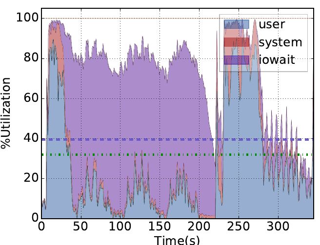
Determining the right cloud configuration for analyt-      performance configuration (within 10% of optimal) with
ics applications is challenging. Even if we limit our-         94% probability and a near-optimal cost configuration
selves to a single instance type and focus on optimizing       with 80% probability. We also analyze Selecta’s sensi-
performance, the choice of storage configuration for a         tivity to various parameters such as the amount of in-
particular application remains non-trivial. Figure 1 com-      formation available for training workloads or the target
pares the performance of three Spark applications using        application.
8 i3.xl AWS instances with l-NVMe, r-SSD, and a hy-               A key contribution of our work is our analysis of cloud
brid (r-SSD for input/output data, l-NVMe for interme-         storage systems and their use by analytics workloads,
diate data). The first application is I/O-bound and bene-      which leads to several important insights. We find that in
fits from the high throughput of NVMe Flash. The sec-          addition to offering the best performance, NVMe-based
ond application has a CPU bottleneck and thus performs         configurations also offer low execution cost for a wide
the same with all three storage options. The third ap-         range of applications. We observe the need for cloud
plication is I/O-bound and performs best with the hybrid       storage options that support fine-grain allocation of ca-
storage option since it minimizing interference between        pacity and bandwidth, similar to the fine-grain allocation
read and write I/Os, which have asymmetric performance         of compute and memory resources offered by serverless
on Flash [40]. This result should not be surprising. An-       cloud services [7]. Disaggregated NVMe Flash can pro-
alytics workloads access multiple data streams, includ-        vide the substrate for such a flexible option for cloud stor-
ing input and output files, logs, and intermediate data        age. Finally, we showcase the need for end-to-end opti-
(e.g., shuffle and broadcast). Each data stream has dis-       mization of cloud storage, including application frame-
tinct characteristics in terms of access frequency, access     works, operating systems, and cloud services, as several
patterns, and data lifetime, which make different streams      storage configurations fail to meet their potential due to
more suitable for different types of storage devices. For      inefficiencies in the storage stack.
example, for TPC-DS query 80 in Figure 1, storing in-
put/output data on r-SSD and intermediate data on l-
NVMe Flash outperforms storing all data on l-NVMe as
                                                               2     Motivation and Background
it isolates streams and eliminates interference.               We discuss current approaches for selecting a cloud stor-
    We present Selecta, a tool that learns near-optimal VM     age configuration and explain the challenges involved.
and storage configurations for analytics applications for
user-specified performance-cost objectives. Selecta tar-
gets analytics jobs that are frequently or periodically re-    2.1    Current Approaches
run on newly arriving data [1, 25, 55]. A configuration        Conventional configurations: Input/output files for data
is defined by the type of cloud instance (core count and       analytics jobs are traditionally stored in a distributed file
memory capacity) along with the storage type and capac-        system, such as HDFS or object storage systems such
ity used for input/output data and for intermediate data.      as Amazon S3 [62, 6]. Intermediate data is typically
To predict application performance for different config-       read/written to/from a dedicated local block storage vol-
urations, Selecta applies latent-factor collaborative fil-     ume on each node (i.e., l-SSD or l-NVMe) and spilled to
tering, a machine-learning technique commonly used in          r-HDD if extra capacity is needed. In typical Spark-as-a-
recommender systems [10, 57, 11, 22, 23]. Selecta uses         service cloud deployments, two remote storage volumes
sparse performance data for training applications profiled     are provisioned by default per instance: one for the in-
on various cloud configurations, as well as performance        stance root volume and one for logs [19].
measurements for the target application profiled on only          Existing tools: Recent work focuses on automat-
two configurations. Selecta leverages the sparse training      ically selecting an optimal VM configuration in the
data to learn significantly faster and more cost-effectively   cloud [71, 69, 3]. However, these tools tend to ignore
than exhaustive search. The approach also improves on          the heterogeneity of cloud storage options, at best distin-
recent systems such as CherryPick and Ernest whose per-        guishing between ‘fast’ and ‘slow’. In the next section,
formance prediction models require more information            we discuss the extent of the storage configuration space.
about the target application and hence require more ap-
plication runs to converge [3, 69]. Moreover, past work
does not consider the heterogeneous cloud storage op-          2.2    Challenges
tions or the varying preferences of different data streams     Complex configuration space: Cloud storage comes in
within each application [71].                                  multiple flavors: object storage (e.g., Amazon S3 [6]),
    We evaluate Selecta with over one hundred Spark SQL        file storage (e.g., Azure Files [45]), and block storage
and ML workloads, each with two different dataset scal-        (e.g., Google Compute Engine Persistent Disks [29]).
ing factors. We show that Selecta chooses a near-optimal       Block and object storage are most commonly used for

760   2018 USENIX Annual Technical Conference                                                        USENIX Association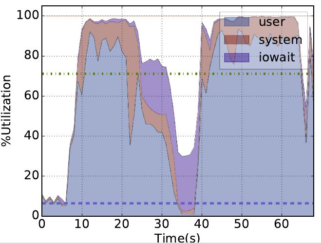
120                                                             5
data analytics. Block storage is further sub-divided into                                                                 Performance
hardware options: cold or throughput-optimized hard                     100                                                             4
                                                                                                                          Cost

                                                               Execution Time (min)

                                                                                                                                            Execution Cost ($)
drive disk, SAS SSD, or NVMe Flash. Block storage can                                 80
                                                                                                                                        3
be local (directly attached) or remote (over the network)                             60
                                                                                                                                        2
to an instance. Local block storage is ephemeral; data                                40
persists only as long as the instance is running. Remote                              20                                                1

volumes persist until explicitly deleted by the user.                                  0                                                0
   Table 1 compares three block storage options available
in Amazon Web Services (AWS). Each storage option
provides a different performance, cost, and flexibility
trade-off. For instance, l-NVMe storage offers the high-
est throughput and lowest latency at higher cost per bit.      Figure 2: Comparison of execution time and cost for
Currently, cloud providers typically offer NVMe in fixed       TPC-DS query 64 on various VM and storage configu-
capacity units directly attached to select instance types,     rations, defined as .
$0.023 more per hour for an instance with 475 GB of
NVMe Flash compared to without NVMe. In contrast,              ples of intermediate data include shuffle data exchanged
S3 fees are based on capacity ($0.023 per GB/month)            between mappers and reducers, broadcast variables, and
and bandwidth ($0.004 per 10K GET requests) usage.             cached dataset partitions spilled from memory. These
   In addition to the storage configuration, users must        streams typically have distinct access frequency, data
choose from a variety of VM types to determine the right       lifetime, access type (random vs. sequential), and I/O
number of CPU cores and memory, the number of VMs,             size. For example, input/output data is generally long-
and their network bandwidth. These choices often af-           lived and sequentially accessed, whereas intermediate
fect storage and must be considered together. For ex-          data is short-lived and most accesses are random.
ample, on instances with 1 Gb/s network bandwidth, the            Storage decisions are complex: Selecting the right
network limits the sequential throughput achievable with       configuration for a job significantly reduces execution
r-HDD and r-SSD storage volumes in Table 1.                    time and cost, as shown in Figure 2, which compares
   Performance-cost objectives: While configurations           a Spark SQL query (TPC-DS query 64) on various VM
with the most CPU cores, the most memory, and fastest          and storage configurations in an 8-node cluster. We con-
storage generally provide the highest performance, opti-       sider 3 i3 VM instance sizes in EC2 (xl, 2xl, and
mizing for runtime cost is much more difficult. Systems        4xl) and heterogeneous storage options for input/output
designed to optimize a specific objective (e.g., predict the   and intermediate data. The lowest performing configura-
configuration that maximizes performance or minimizes          tion has 24× the execution time of the best performing
cost) are generally not sufficient to make recommenda-         configuration. Storing input/output data on r-SSD and
tions for more complex objectives (e.g., predict the con-      intermediate data on l-NVMe (the lowest cost configura-
figuration that minimizes execution time within a spe-         tion) has 7.5× lower cost than storing input/output data
cific budget). By predicting application execution time        on r-HDD and intermediate data on r-SSD.
on candidate configurations, our approach remains gen-
eral. Unless otherwise specified, we refer to cost as the
                                                               3                           Selecta Design
cost of executing an application.
   Heterogeneous application data: We classify data            3.1                          Overview
managed by distributed data analytics frameworks (e.g.,
Spark [74]) into two main categories: input/output data        Selecta is a tool that automatically predicts the perfor-
which is typically stored long-term and intermediate           mance of a target application on a set of candidate con-
data which lives for the duration of job execution. Exam-      figurations. As shown in Figure 3, Selecta takes as in-
                                                               put: i) execution time for a set of training applications
                                                               on several configurations, ii) execution time for the tar-
 Storage     Seq      Seq       Rand      Rand     Rand        get application on two reference configurations, and iii) a
             Read     Write     Read      Write    Rd/Wr
             MB/s     MB/s      IOPS      IOPS     IOPS        performance-cost objective for the target application. A
 r-HDD         135      135        132       132      132      configuration is defined by the number of nodes (VM in-
 r-SSD         165      165      3,068     3,068    3,068      stances), the CPU cores and memory per node, as well as
 l-NVMe        490      196    103,400    35,175   70,088      the storage type and capacity used for input/output data
Table 1: Block storage performance for 500GB vol-              and for intermediate data. Selecta uses latent factor col-
umes. Sequential IOs are 128 KB, random IOs are 4 KB.          laborative filtering (see §3.2) to predict the performance

USENIX Association                                                                          2018 USENIX Annual Technical Conference     761
SELECTA
Training configurations
Training
App
Training Profile on 20%
App
Training 2 … 2 1 2 2 … 2 1
App of configs
App 8 … 1 5 8 … 3 1
applications
…
…
… …
SVD
… 5 1 1 4 … 5 1 Recommended
Target Profile on 2 2 3 … 1 2 3 … 7 1 VM & storage
App reference configs 5 2 … 4 1
configuration
2 1
performance
prediction
Rank configs
Perf/Cost
Objective Run recommended feedback
config update
e.g., minimize cost
Figure 3: An overview of performance prediction and configuration recommendation with Selecta.
of the target application on the remaining (non-reference) CherryPick [3] and Ernest [69] build performance mod-
candidate configurations. With these performance pre- els based solely on training data for the target applica-
dictions and the per unit time cost of various VM in- tion, Selecta’s goal is to leverage training data available
stances and storage options, Selecta can recommend the from multiple applications to converge to accurate rec-
right configuration for the user’s performance-cost ob- ommendations with only two profiling runs of a target
jective. For example, Selecta can recommend configu- application. We discuss alternatives to collaborative fil-
rations that minimize execution time, minimize cost, or tering to explain our choice.
minimize execution time within a specific budget. Content-based approaches, such as as linear regres-
As new applications are launched over time, these per- sion, random forests, and neural network models, build
formance measurements become part of Selecta’s grow- a model from features such as application characteris-
ing training set and accuracy improves (see § 4.4). We tics (e.g., GB of shuffle data read/written) and configu-
also feed back performance measurements after running ration characteristics (e.g., I/O bandwidth or the num-
a target application on a configuration recommended by ber of cores per VM). We find that unless inputs fea-
Selecta — this helps reduce measurement noise and im- tures such as the average CPU utilization of the target
prove accuracy. Since Selecta takes ∼1 minute to gen- application on the target configuration are used in the
erate a new set of predictions (the exact runtime de- model, content-based predictors do not have enough in-
pends on the training matrix size), a user can re-run Se- formation to learn the compute and I/O requirements of
lect when re-launching the target application with a new applications and achieve low accuracy. Approaches that
dataset to get a more accurate recommendation. In our require running target applications on all candidate con-
experiments, the recommendations for each target appli- figurations to collect feature data are impractical.
cation converge after two feedback iterations. The ability
to grow the training set over time also provides Selecta Another alternative is to build performance prediction
with a mechanism for expanding the set of configurations models based on the structure of an analytics frame-
it considers. Initially, the configuration space evaluated work, such as the specifics of the map, shuffle, and re-
by Selecta is the set of configurations that appear in the duce stages in Spark [36, 75]. This leads to framework-
original training set. When a new configuration becomes specific models and may require re-tuning or even re-
available and Selecta receives profiling data for applica- modeling as framework implementations evolve (e.g., as
tions on this configuration, the tool will start predicting the CPU efficiency of serialization operations improves).
performance for all applications on this configuration. Latent factor collaborative filtering: Selecta’s col-
laborative filtering model transforms applications and
configurations to a latent factor space [10]. This space
3.2 Predicting Performance
characterizes applications and configurations in terms of
Prediction approach: Selecta uses collaborative filter- latent (i.e., ‘hidden’) features. These features are auto-
ing to predict the performance of a target application on matically inferred from performance measurements of
candidate configurations. We choose collaborative filter- training applications [56]. We use a matrix factoriza-
ing as it is agnostic to the details of the data analytics tion technique known as Singular Value Decomposition
framework used (e.g., Spark vs. Storm) and it allows us (SVD) for the latent factor model. SVD decomposes an
to leverage sparse training data collected across appli- input matrix P, with rows representing applications and
cations and configurations [56]. While systems such as columns representing configurations, into the product of
762 2018 USENIX Annual Technical Conference USENIX Associationthree matrices, U, λ , and V . Each element pi j of P rep- Adapting to changes: Recurring jobs and their input
resents the normalized performance of application i on datasets are likely to evolve. To detect changes in appli-
configuration j. The latent features are represented by cation characteristics that may impact the choice of op-
singular values in the diagonal matrix λ , ordered by de- timal configuration, Selecta relies on CPU utilization in-
creasing magnitude. The matrix U captures the strength formation from both initial application profiling and sub-
of the correlation between a row in P and a latent feature sequent executions rounds. When an application is first
in λ . The matrix V captures the strength of the corre- introduced to the system, Selecta assigns a unique ID to
lation between a column in P and a latent feature in λ . store application specific information such as iowait CPU
Although the model does not tell us what the latent fea- utilization. Whenever an application is re-executed, Se-
tures physically represent, a hypothetical example of a lecta compares the current iowait time to the stored con-
latent feature is random I/O throughput. For instance, figuration. Depending on the difference in iowait time,
Selecta could infer how strongly an application’s perfor- Selecta will either compute a refined prediction based on
mance depends on random I/O throughput and how much available measurements or treat the workload as new ap-
random I/O throughput a configuration provides. plication, starting a new profiling run.
One challenge for running SVD is the input matrix P Dealing with noise in the cloud: An additional chal-
is sparse, since we only have the performance measure- lenge for recommending optimal configurations is noise
ments of applications on certain configurations. In par- on public cloud platforms, which arises due to interfer-
ticular, we only have two entries in the target applica- ence with other tenants, hardware heterogeneity, or other
tion row and filling in the missing entries corresponds sources [59]. To account for noise, Selecta relies on the
to predicting performance on the other candidate con- feedback of performance and CPU utilization measure-
figurations. Since performing SVD matrix factorization ments. Initially, with few profiling runs, Selecta’s perfor-
requires a fully populated input matrix P, we start by mance predictions are affected by noise. As more mea-
randomly initializing the missing entries and then run surements are fed into the system, Selecta averages per-
Stochastic Gradient Descent (SGD) to update these un- formance and CPU utilization and uses reservoir sam-
known entries using an objective function that minimizes pling to avoid high skew from outliers [70]. Selecta
the mean squared error on the known entries of the ma- keeps a configurable number of sample points for each
trix [13]. The intuition is that by iteratively decompos- entry in the application-configuration matrix (e.g., three)
ing and updating the matrix in a way that minimizes the to detect changes in applications as described above.
error for known entries, the technique also updates un- If a particular run is heavily impacted by noise such
known entries with accurate predictions. Selecta uses the that the compute and I/O bottlenecks differ significantly
Python sci-kit surprise library for SVD [33]. from previous runs, Selecta’s mechanism for detecting
changes in applications identifies the outlier.
3.3 Using Selecta
New target application: The first time an application is 4 Selecta Evaluation
presented to Selecta, it is profiled on two reference con-
figurations which, preferably, are far apart in their com- Selecta’s collaborative filtering approach is agnostic to
pute and storage resource attributes. Selecta requires that the choice of applications and configurations. We evalu-
reference configurations remain fixed across all applica- ate Selecta for data analytics workloads on a subset of the
tions, since performance measurements are normalized cloud configuration space with the goal of understanding
to a reference configuration before running SVD. Profil- how to provision cloud storage for data analytics.
ing application performance involves running the appli-
cation to completion and recording execution time and
4.1 Methodology
CPU utilization (including iowait) over time.
Defining performance-cost objectives: After pre- Cloud configurations: We deploy Selecta on Amazon
dicting application performance across all configura- EC2 and consider configurations with the instance and
tions, Selecta recommends a configuration based on a storage options shown in Tables 2 and 3. Among the
user-defined ranking function. For instance, to mini- possible VM and storage combinations, we consider sev-
mize runtime cost, the ranking function is min(runtime enteen candidate configurations. We trim the space to
× cost/hour). While choosing a storage technology stay within our research budget and to focus on experi-
(e.g., SSD vs. NVMe Flash), Selecta must also consider ments that are most likely to uncover interesting insights
the application’s storage capacity requirements. Selecta about cloud storage for analytics. We choose EC2 in-
leverages statistics from profiling runs available in Spark stance families that are also supported by Databricks, a
monitoring logs to determine the intermediate (shuffle) popular Spark-as-a-service provider [18]. i3 is currently
data and and input/output data capacity [63]. the only instance family available with NVMe Flash and
USENIX Association 2018 USENIX Annual Technical Conference 763Instance CPU cores RAM (GB) NVMe
i3.xlarge 4 30 1 x 950 GB 14, 16, 21, 26, 28, 29. We also run 100 and 400 GB
r4.xlarge 4 30 - sort jobs [52]. Finally, we run a SQL equijoin query on
i3.2xlarge 8 60 1 x 1.9 TB
r4.2xlarge 8 60 -
two tables with 16M and 32M rows each and 4KB en-
i3.4xlarge 16 120 2 x 1.9 TB tries [53]. For all input and output files, we use the un-
r4.4xlarge 16 120 - compressed Parquet data format [26].
Table 2: AWS instance properties Experiment methodology: We run each application
on all candidate configurations to obtain the ground truth
Use for Use for performance and optimal configuration choices for each
Storage Type Locality Input/Output Intermediate application. To account for noise in the cloud we run
Data? Data?
r-HDD Block Remote X - each experiment (i.e., each application on each candidate
r-SSD Block Remote X X configuration) three times and use the average across
l-NVMe Block Local X X runs in our evaluation. Two runs are consecutive and one
S3 Object Remote X -
run is during a different time of day. We also validate our
Table 3: AWS storage options considered results by using data from one run as input to Selecta and
the average performance across runs as the ground truth.
To train and test Selecta, we use leave-one-out cross val-
r4 instances allow for a fair comparison of storage op- idation [58], meaning one workload at a time serves as
tions as they have the same memory to compute ratio. the target application while the remaining workloads are
We only consider configurations where the intermediate used for training. We assume training applications are
data storage IOPS are equal to or greater than the in- profiled on all candidate configurations, except for the
put/output storage IOPS, as intermediate data has more sensitivity analysis in §4.4 where we investigate training
random accesses. Since we find that most applications matrix density requirements for accurate predictions.
are I/O-bound with r-HDD, we only consider r-HDD for Metrics: We measure the quality of Selecta’s predic-
the instance size with the least amount of cores. We limit tions using two metrics. First, we report the relative root
our analysis to r-HDD because our application datasets mean squared error (RMSE), a common metric for rec-
are up to 1 TB whereas instances with l-HDD on AWS ommender systems. The second and more relevant met-
come with a minimum of 6 TB disk storage, which would ric for Selecta is the probability of making an accurate
not be an efficient use of capacity. We do not consider configuration recommendation. We consider a recom-
local SAS/SATA SSDs as their storage capacity to CPU mendation accurate if the configuration meets the user’s
cores ratio is too low for most Spark workloads. We use cost-performance objective within a threshold T of the
Elastic Block Store (EBS) for remote block storage [5]. true optimal configuration for that application. For ex-
We use a cluster of 9 nodes for our evaluation. The ample, for a minimum cost objective with T = 10%, the
cluster consists of one master node and eight executor probability of an accurate prediction is the percentage
nodes. The master node runs the Spark driver and YARN of Selecta’s recommendations (across all tested applica-
Resource Manager. Unless input/output data is stored in tions) whose true cost is within 10% of the true optimal
S3, we run a HDFS namenode on the master server as cost configuration. Using a threshold is more robust to
well. We configure framework parameters, such as the noise and allows us to make more meaningful conclu-
JVM heap size and number of executors, according to sions about Selecta’s accuracy, since a second-best con-
Spark tuning guidelines and match the number of execu- figuration may have similar or significantly worse per-
tor tasks to the VM’s CPU cores [15, 14]. formance than the best configuration. Our performance
Applications: We consider Spark [74] as a represen- metric is execution time and cost is in US dollars.
tative data analytics framework, similar to previous stud-
ies [50, 68, 3]. We use Spark v2.1.0 and Hadoop v2.7.3 4.2 Prediction Accuracy
for HDFS. We evaluate Selecta with over one hundred
Spark SQL and ML applications, each with two different We provide a matrix with 204 rows as input to Selecta,
dataset scales, for a total of 204 workloads. Our appli- where one row (application) is designated as the target
cation set includes 92 queries of the TPC-DS benchmark application in each test round. We run Selecta 204 times,
with scale factors of 300 and 1000 GB [67]. We use the each time considering a different application as the tar-
same scale factors for Spark SQL and ML queries from get. For now, we assume all remaining rows of train-
the TPC-BB (BigBench) benchmark which has of struc- ing data in the matrix are dense, implying the user has
tured, unstructured and semi-structured data modeled af- profiled training applications on all candidate configu-
ter the retail industry domain [27]. Since most BigBench rations. The single target application row is sparse, con-
queries are CPU-bound, we focus on eight queries which taining only two entries, one for each of the profiling runs
have more substantial I/O requirements: queries 3, 8, on reference configurations.
764 2018 USENIX Annual Technical Conference USENIX Associationperf-predict-using-small
cost-predict-using-small
cost*perf-predict-using-small
perf-predict-using-large
cost-predict-using-large
cost*perf-predict-using-large
Figure 4: Probability of accurate Figure 5: Probability of accu- Figure 6: Accuracy with large
recommendations within a thresh- rate configuration recommendation datasets using predictions from
old from optimal. Dotted lines are for performance within threshold, small dataset vs. re-computing pre-
after one feedback iteration. given strict cost restrictions. diction with large dataset.
Selecta predicts performance with a relative RMSE urations (i.e., cases where Selecta recommends a config-
of 36%, on average across applications. To understand uration that is actually over budget).
how Selecta’s performance predictions translate into rec- In Figure 7, we compare Selecta’s accuracy against
ommendations, we plot accuracy in Figure 4 for perfor- four baselines. The first baseline is a random forest pre-
mance, cost and cost*performance objectives. The plot dictor, similar to the approach used by PARIS [71]. We
shows the probability of near-optimal recommendations use the following features: the number of CPU cores,
as a function of the threshold T defining what percentage disk IOPS and disk MB/s the configuration provides, the
from optimal is considered close enough. When search- intermediate and input/output data capacity of the appli-
ing for the best performing configuration, Selecta has a cation, and the CPU utilization, performance, and total
94% probability of recommending a configuration within disk throughput measured when running the application
10% of optimal. For a minimum cost objective, Selecta on each of the two reference configurations. Although
has a 80% probability of recommending a configuration the random forest predictor leverages more features than
within 10% of optimal. Predicting cost*performance is Selecta, it has lower accuracy. Collaborative filtering
more challenging since errors in Selecta’s relative execu- is a better fit for the sparse nature of the training data.
tion time predictions for an application across candidate We find the most important features in the random for-
configurations are squared: cost*performance = (execu- est model are all related to I/O (e.g., the I/O throughput
tion time)2 * config cost per hour. measured when running the application on the reference
The dotted lines in Figure 4 show how accuracy im- configurations and the read/write IOPS supported by the
proves after a single feedback round. Here, we assume storage used for intermediate data), which emphasizes
the target application has the same dataset in the feed- the importance of selecting the right storage.
back round. This provides additional training input for The second baseline (labeled ‘default’) in Figure 7
the target application row (either a new entry if the rec- uses the recommended default configurations docu-
ommended configuration was not a reference configura- mented in Databricks engineering blog posts: l-NVMe
tion, or a new sample to average to existing data if the for intermediate data and S3 for input/output data [19,
recommended configuration was a reference configura- 21, 20]. The ‘max cost per time’ baseline uses the simple
tion). The probability of near-optimal recommendations heuristic of always picking the most expensive instance
increases most noticeably for the cost*performance ob- per unit time. The ’min cost per time’ baseline chooses
jective, from 52% to 65% after feedback, with T =10%. the least expensive instance per unit time. Selecta out-
Figure 5 shows the probability of accurate recommen- performs all of these heuristic strategies, confirming the
dations for objectives of the form “select the best per- need for a tool to automate configuration selection.
forming configuration given a fixed cost restriction C.”
For this objective, we consider Selecta’s recommenda- 4.3 Evolving Datasets
tion accurate if its cost is less than or equal to the budget
and if its performance is within the threshold of the true We study the impact of dataset size on application per-
best configuration for the objective. Selecta achieves be- formance and Selecta’s predictions using the small and
tween 83% and 94% accuracy for the cost restrictions in large dataset scales described in §4.1. We train Selecta
Figure 5 assuming T =10%. The long tail is due to per- using all 102 workloads with small datasets, then evalu-
formance prediction errors that lead Selecta to underesti- ate Selecta’s prediction accuracy for the same workloads
mate the execution cost for a small percentage of config- with large datasets. The dotted lines in Figure 6 plots Se-
USENIX Association 2018 USENIX Annual Technical Conference 765lecta’s accuracy when recommending configurations for
applications with large datasets solely based on profil-
ing runs of the application with a smaller dataset. The
solid lines show accuracy when Selecta re-profiles appli-
cations with large datasets to make predictions. For ap-
proximately 8% of applications, profiling runs with small
datasets are not sufficient indicators of performance with
large datasets.
We find that in cases where the performance with a
small dataset is not indicative of performance with a
large dataset, the relationship between compute and I/O
Figure 7: Selecta’s accuracy compared to baselines.
intensity of the application is affected by the dataset size.
As described in §3.3, Selecta detects these situations by
comparing CPU utilization statistics for the small and
large dataset runs. Figure 8 shows an example of a work-
load for which small dataset performance is not indica-
tive of performance with a larger dataset. We use the
Intel Performance Analysis Tool to record and plot CPU
utilization [34]. When the average iowait percentage for
the duration of the run changes significantly between the
large and small profiling runs on the reference configura-
(a) Query on 300GB is CPU-bound. (b) Query on 1TB is IO-bound.
tion, it is generally best to profile the application on the
reference configurations and treat it as a new application.
Figure 8: CPU utilization over time for TPC-DS query
89 on r4.xlarge cluster with r-SSD. For this query,
4.4 Sensitivity Analysis performance with a small dataset is not indicative of per-
formance with a larger dataset. Selecta detects difference
We perform a sensitivity analysis to determine input ma- in average iowait percentage (blue dotted line).
trix density requirements for accurate predictions. We
look at both the density of matrix rows (i.e., the percent-
age of candidate configurations that training applications racy does not depend on a training application directly
are profiled on) and the density of matrix columns (i.e., related to the target application. Since the number of
the number of training applications used). We also dis- training applications required to achieve desirable accu-
cuss sensitivity to the choice of reference configurations. racy depends on the size of the configuration space a user
Figure 9a shows how Selecta’s accuracy for perfor- wishes to explore, the x-axis in Figure 9b represents the
mance, cost and cost*performance objectives varies as a ratio of the number of training applications to the number
function of input matrix density. Assuming 203 training of candidate configurations, R. We find that to jump start
applications have accumulated in the system over time, Selecta with dense training data from a cold start, users
we show that, on average across target applications, rows should provide 2.5× more training applications than the
only need to be approximately 20 to 30% dense for Se- number of candidate configurations to achieve desirable
lecta to achieve sufficient accuracy. This means that at accuracy. In our case, jump starting Selecta with more
steady state, users should profile training applications on than 43 = d2.5 × 17e training applications profiled on all
about 20-30% of the candidate configurations (including 17 configurations reaches a point of diminishing returns.
reference configurations). Profiling additional configura- Finally, we investigate whether, a cold start requires
tions has diminishing returns. profile training applications on all configurations. We
Next, we consider a cold start situation in which a user use R=2.5, which for 17 candidate configurations corre-
wants to jump start the system by profiling a limited set sponds to using 43 training applications. Figure 9c plots
of training applications across all candidate configura- accuracy as we vary the percentage of candidate config-
tions. Figure 9b shows the number of training applica- urations on which the training applications are profiled
tions required to achieve desired accuracy. Here, for each (including reference configurations, which we assume
target application testing round, we take the 203 training are always profiled). The figure shows that for a cold
applications we have and randomly remove a fraction of start, it is sufficient for users to profile the initial train-
the rows (training applications). We ensure to drop the ing applications on 40% to 60% of candidate configu-
row corresponding to the different dataset scale factor rations. As Selecta continues running and accumulates
run of the target application, to ensure Selecta’s accu- more training applications, the percentage of configura-
766 2018 USENIX Annual Technical Conference USENIX Association(a) Sensitivity to input matrix density in (b) Sensitivity to number of training ap- (c) Sensitivity to input matrix density for
steady state: 20% density per row suffices plications, profiled on all configurations: cold start: ∼50% density per row (train-
for accurate predictions. 2.5× the number of configs suffices. ing application) required.
Figure 9: Sensitivity analysis: accuracy as a function of input matrix density
tions users need to profile for training applications drops time by a median of at most 19% [50]. We believe the
to 20-30% (this is the steady state result from Figure 9a). main reason for the increased impact of storage on end-
We experimented with different reference configura- to-end application performance is due to the newer ver-
tions for Selecta. We find that accuracy is not very sen- sion of Spark we use in our study (v2.1.0 versus v1.2.1).
sitive to the choice of references. We saw a slight bene- Spark has evolved with numerous optimizations target-
fit using references that have different VM and storage ing CPU efficiency, such as cache-aware computations,
types. Although one reference configuration must re- code generation for expression evaluation, and serializa-
main fixed across all application runs since it is used to tion [17]. With ongoing work in optimizing the CPU
normalize performance, we found that the reference con- cycles spent on data analytics computations, for example
figuration used for the second profiling run could vary by optimizing the I/O processing path [66], we expect
without significant impact on Selecta’s accuracy. the choice of storage to be of even greater importance.
The need for flexible capacity and bandwidth allo-
cation: Provisioning storage involves selecting the right
5 Cloud Storage Insights capacity, bandwidth, and latency. Selecta uses statistics
from Spark logs to determine capacity requirements and
Our analysis of cloud configurations for data analytics applies collaborative filtering to explore performance-
reveals several insights for cloud storage configurations. cost trade-offs. However, the cost-efficiency of the stor-
We discuss key takeaways and their implications for fu- age configuration selected is limited by numerous con-
ture research on storage systems. straints imposed by cloud providers. For example, for re-
NVMe storage is performance and cost efficient for mote block storage volumes, the cloud provider imposes
data analytics: We find that configurations with NVMe minimum capacity limits (e.g., 500 GB for r-HDD on
Flash tend to offer not only the best performance, but AWS) and decides how data in the volume is mapped to
also, more surprisingly, the lowest cost. Although NVMe physical devices, which directly affects storage through-
Flash is the most expensive type of storage per GB/hr, its put (e.g., HDD throughput is proportional to the number
high bandwidth allows applications to run significantly of spindles). A more important restriction is for local
faster, reducing the overall job execution cost. storage, such as l-NVMe, which is only available in fixed
On average across applications, we observe that l- capacities attached to particular instance types. The fixed
NVMe Flash reduces job completion time of applica- ratio between compute, memory and storage resources
tions by 27% compared to r-SSD and 75% compared to imposed by cloud vendors does not provide the right bal-
r-HDD. Although we did not consider l-SSD or l-HDD ance of resources for many of the applications we stud-
configurations in our evaluation, we validate that local ied. For example the SQL equijoin query on two 64 GB
versus remote access to HDD and SDD achieves simi- tables saturates the IOPS of the 500 GB NVMe device on
lar performance since our instances have sufficient net- a i3.xl instance, but leaves half the capacity underuti-
work bandwidth (up to 10 Gb/s) and modern networking lized. Furthermore, local storage is ephemeral, meaning
adds little overhead on top of HDD and SSD access la- instances must be kept on to retain data on local devices.
tency [8]. In contrast, a previous study of Spark applica- Thus, although we showed it is cost-efficient to store in-
tions by Ousterhout et al. concluded that optimizing or put/output and intermediate data on l-NVMe for the du-
eliminating disk accesses can only reduce job completion ration of a job, storing input/output files longer term on
USENIX Association 2018 USENIX Annual Technical Conference 767l-NVMe would dramatically increase cost compared to reads overlapped with large shuffle writes, such as for using remote storage volumes or an object storage sys- TPC-DS query 80 shown in Figure 1. A disaggregated tem such as S3. Flash storage system must address interference using ei- We make the case for a fast and flexible storage op- ther scheduling approaches [40, 47, 61, 51, 60] or device- tion in the cloud. Emerging trends in cloud comput- level isolation mechanisms [12, 54, 38]. Finally, the are ing, such as serverless computing offerings like AWS interesting trade-offs in the interfaces used to expose dis- Lambda, Google Cloud Functions and Azure Functions, aggregated Flash (e.g., block storage, key-value storage, provide fine-grain, pay-per-use access to compute and distributed file system, or other). memory resources [31, 7, 28, 46]. Currently, there is no The need for end-to-end optimization: In our ex- option that allows for fine-grain capacity and bandwidth periments, remote HDD storage performed poorly, de- allocation of cloud storage with low latency and high spite its cost effectiveness for long-living input/output bandwidth characteristics [41]. Although S3 provides data and its ability to match the sequential bandwidth of- pay-per-use storage with high scalability, high availabil- fered by SSD. Using the Linux blktrace tool [37] to ity and relatively high bandwidth, we show that data an- analyze I/O requests at the block device layer, we found alytics applications benefit from even higher throughput that although each Spark task reads/writes input/output (i.e., NVMe Flash). S3 also incurs high latency, which data sequentially, streams from multiple tasks running on we observed to be a major bottleneck for short-running different cores interleave at the block device layer. Thus, SQL queries that read only a few megabytes of data. the access stream seen by a remote HDD volume consists Disaggregated NVMe is a promising option for of approximately 60% random I/O operations, dramati- fast and flexible cloud storage: Disaggregating NVMe cally reducing performance compared to fully sequen- Flash by enabling efficient access to the resource over tial I/O. This makes solutions with higher throughput for the network is a promising option for fast and flexi- random accesses (e.g., using multiple HDDs devices or ble cloud storage. Recent developments in hardware- Flash storage) more appropriate for achieving high per- assisted [49, 44] and software-only [40] techniques en- formance in data analytics. Increasing random I/O per- able access to remote NVMe devices with low latency formance comes at a higher cost per unit time. In addi- overheads over a wide range of network options, includ- tion to building faster storage systems, we should attempt ing commodity Ethernet networking with TCP/IP pro- to optimize throughout the stack for sequential accesses tocols. These techniques allow us to build disaggre- when these accesses are available at the application level. gated Flash storage that allows fine-grain capacity and Of course, there will always be workloads with intrinsi- IOPS allocation for analytics workloads and independent cally random access patterns that will not benefit from scaling of storage vs. compute resources. Applications such optimizations. would allocate capacity and bandwidth on demand from a large array of remotely accessible NVMe devices. In 6 Discussion this setting, Selecta can help predict the right capacity and throughput requirements for each data stream in an Our work focused on selecting storage configurations analytics workload to guide the allocation of resources based on their performance and cost. Other impor- from a disaggregated Flash system. tant considerations include durability, availability, and There are several challenges in implementing flexi- consistency, particularly for long-term input/output data ble cloud storage based on disaggregated Flash. First, storage [42]. Developers may also prefer a particular networking requirements can be high. Current NVMe storage API (e.g., POSIX files vs. object interface). devices on AWS achieve 500 MB/s to 4 GB/s sequen- Users can use these qualitative constraints to limit the tial read bandwidth, depending on the capacity. Write storage space Selecta considers. Users may also choose throughput and random access bandwidth is also high. different storage systems for high performance process- The networking infrastructure of cloud systems must be ing versus long term storage of important data. able to support a large number of instances accessing Our study showed that separating input/output data NVMe Flash remotely with the ability to burst to the and intermediate data uncovers a richer configuration maximum throughput of the storage devices. An addi- space and allows for better customization of storage re- tional challenge with sharing remote Flash devices is in- sources to the application requirements. We can further terference between read and write requests from differ- divide intermediate data into finer-grained streams such ent tenants [40, 61]. We observed several cases where as shuffle data, broadcast data, and cached RDDs spilled separating input/output data and intermediate data on r- from memory. Understanding the characteristics of these SSD (or S3) and l-NVMe, respectively, led to higher finer grain streams and how they should be mapped to performance (and lower cost) than storing all data on l- storage options in the cloud may reveal further benefits. NVMe. This occurred for jobs where large input data Compression schemes offer an interesting trade-off 768 2018 USENIX Annual Technical Conference USENIX Association
between processing, networking, and storage require-              Automating storage configurations: Many previ-
ments. In addition to compressing input/output files, sys-     ous systems provide storage configuration recommen-
tems like Spark allow compressing individual interme-          dations [9, 65, 2, 48, 4, 30, 39]. Our work analyzes
diate data streams using a variety of compression algo-        the trade-offs between traditional block storage and ob-
rithms (lz4, lzf, and snappy) [64]. In future work, we         ject storage available in the cloud. We also considering
plan to extend Selecta to consider compression options         how heterogeneous streams in data analytics applications
in addition to storage and instance configuration.             should be mapped to heterogeneous storage options.
   We used Selecta to optimize data analytics applica-            Analyzing performance of analytics frameworks:
tions as they represent a common class of cloud work-          While previous studies analyze how CPU, memory,
loads. Selecta’s approach should be applicable to other        network and storage resources affect Spark perfor-
data-intensive workloads too, as collaborative filtering       mance [50, 68, 66, 43], our work is the first to evalu-
does not make any specific assumptions about the appli-        ate the impact of new cloud storage options (e.g., NVMe
cation structure. In addition to considering other types       Flash) and provide a tool to navigate the diverse storage
of workloads, in future work, we will consider scenarios       configuration space.
in which multiple workloads share cloud infrastructure.           Tuning application parameters: Previous work
Delimitrou et al. have shown that collaborative filter-        auto-tunes data analytics framework parameters such as
ing can classify application interference sensitivity (i.e.,   the number of executors, JVM heap size, and compres-
how much interference an application will cause to co-         sion schemes [32, 73, 72]. Our work is complementary.
scheduled applications and how much interference it can        Users set application parameters and then run Selecta to
tolerate itself) [22, 23]. We also believe Selecta’s collab-   obtain a near-optimal hardware configuration.
orative filtering approach can be extended to help con-
figure isolation mechanisms that limit interference be-        8   Conclusion
tween workloads, particularly on shared storage devices
like NVMe which exhibit dramatically different behavior        The large and increasing number of storage and com-
as the read-write access patterns vary [40].                   pute options on cloud services makes configuring data
                                                               analytics clusters for high performance and cost effi-
                                                               ciency difficult. We presented Selecta, a tool that learns
7   Related Work                                               near-optimal configurations of compute and storage re-
                                                               sources based on sparse training data collected across
Selecting cloud configurations: Several recent sys-
                                                               applications and candidate configurations. Requiring
tems unearth near-optimal cloud configurations for target
                                                               only two profiling runs of the target application, Se-
workloads. CherryPick uses Bayesian Optimization to
                                                               lecta predicts near-optimal performance configurations
build a performance model that is just accurate enough to
                                                               with 94% probability and near-optimal cost configura-
distinguish near-optimal configurations [3]. Model input
                                                               tions with 80% probability. Moreover, Selecta allowed
comes solely from profiling the target application across
                                                               us to analyze cloud storage options for data analytics
carefully selected configurations. Ernest predicts perfor-
                                                               and reveal important insights, including the cost benefits
mance for different VM and cluster sizes, targeting ma-
                                                               of NVMe Flash storage, the need for fine-gain alloca-
chine learning analytics applications [69]. PARIS takes
                                                               tion of storage capacity and bandwidth in the cloud, and
a hybrid online/offline approach, using random forests to
                                                               the need for cross-layer storage optimizations. We be-
predict application performance on various VM config-
                                                               lieve that, as data-intensive workloads grow in complex-
urations based on features such as CPU utilization ob-
                                                               ity and cloud options for compute and storage increase,
tained from profiling [71]. These systems do not con-
                                                               tools like Selecta will become increasingly useful for
sider the vast storage configuration options in the cloud
                                                               end users, systems researchers, and even cloud providers
nor the heterogeneous data streams of analytics applica-
                                                               (e.g., for scheduling ‘serverless’ application code).
tions which can dramatically impact performance.
   Resource allocation with collaborative filtering:
Our approach for predicting performance is most similar        Acknowledgements
to Quasar [23] and Paragon [22], which apply collabora-
tive filtering to schedule incoming applications on shared     We thank our anonymous reviewers as well as Christina
clusters. ProteusTM [24] applies collaborative filtering       Delimitrou, Francisco Romero, and Neeraja Yadwadkar
to auto-tune a transactional memory system. While these        for their feedback. This work is supported by the Stan-
systems consider resource heterogeneity, they focus on         ford Platform Lab, Samsung, Huawei and NSF grant
CPU and memory. While Selecta applies a similar mod-           CNS-1422088. Ana Klimovic is supported by a Stan-
eling approach, our exploration of the cloud storage con-      ford Graduate Fellowship and Microsoft Research PhD
figuration space is novel and reveals important insights.      Fellowship.

USENIX Association                                                   2018 USENIX Annual Technical Conference         769
References ings of the 13th ACM SIGKDD International Con-
ference on Knowledge Discovery and Data Mining
[1] AGARWAL , S., K ANDULA , S., B RUNO , N., W U , (2007), KDD ’07, pp. 95–104.
M.-C., S TOICA , I., AND Z HOU , J. Re-optimizing
data-parallel computing. In Proceedings of the 9th [11] B ELL , R. M., KOREN , Y., AND VOLINSKY, C.
USENIX Conference on Networked Systems Design The BellKor 2008 Solution to the Netflix Prize.
and Implementation (2012), NSDI’12, pp. 21–21. Tech. rep., 2008.
[2] A LBRECHT, C., M ERCHANT, A., S TOKELY, M., [12] B JØRLING , M., G ONZALEZ , J., AND B ONNET,
WALIJI , M., L ABELLE , F., C OEHLO , N., S HI , X., P. Lightnvm: The linux open-channel SSD sub-
AND S CHROCK , C. E. Janus: Optimal flash provi- system. In 15th USENIX Conference on File and
sioning for cloud storage workloads. In Proceed- Storage Technologies (FAST 17) (2017), pp. 359–
ings of the 2013 USENIX Conference on Annual 374.
Technical Conference (2013), USENIX ATC’13,
[13] B OTTOU , L. Large-Scale Machine Learning with
pp. 91–102.
Stochastic Gradient Descent. Physica-Verlag HD,
[3] A LIPOURFARD , O., L IU , H. H., C HEN , J., 2010, pp. 177–186.
V ENKATARAMAN , S., Y U , M., AND Z HANG ,
[14] C LOUDERA. How-to: Tune your apache spark
M. CherryPick: Adaptively unearthing the best
jobs. https://blog.cloudera.com/blog/
cloud configurations for big data analytics. In 14th
2015/03/how-to-tune-your-apache-spark-
USENIX Symposium on Networked Systems De-
jobs-part-2/, 2015.
sign and Implementation (NSDI 17) (Boston, MA,
2017), pp. 469–482. [15] C LOUDERA. Tuning spark applica-
tions. https://www.cloudera.com/
[4] A LVAREZ , G. A., B OROWSKY, E., G O , S.,
documentation/enterprise/5-9-x/topics/
ROMER , T. H., B ECKER -S ZENDY, R., G OLDING ,
admin spark tuning.html, 2017.
R., M ERCHANT, A., S PASOJEVIC , M., V EITCH ,
A., AND W ILKES , J. Minerva: An automated re- [16] C ORPORATION , I. Intel Optane SSD DC
source provisioning tool for large-scale storage sys- P4800X Available Now on IBM Cloud.
tems. ACM Trans. Comput. Syst. 19, 4 (Nov. 2001), https://www.ibm.com/blogs/bluemix/
483–518. 2017/08/intel-optane-ssd-dc-p4800x-
available-now-ibm-cloud, 2017.
[5] A MAZON. Amazon elastic block store (EBS).
https://aws.amazon.com/ebs, 2017. [17] DATABRICKS. Project tungsten: Bring-
ing apache spark closer to bare metal.
[6] A MAZON. Amazon simple storage service. https:
https://databricks.com/blog/2015/04/
//aws.amazon.com/s3, 2017.
28/project-tungsten-bringing-spark-
[7] A MAZON. AWS lambda. https: closer-to-bare-metal.html, 2015.
//aws.amazon.com/lambda, 2017.
[18] DATABRICKS. AWS configurations for Spark.
[8] A NANTHANARAYANAN , G., G HODSI , A., https://docs.databricks.com/user-guide/
S HENKER , S., AND S TOICA , I. Disk-locality in clusters/aws-config.html#ebs-volumes,
datacenter computing considered irrelevant. In 2016.
Proc. of USENIX Hot Topics in Operating Systems
[19] DATABRICKS. Supported instance types.
(2011), HotOS’13, pp. 12–12.
https://databricks.com/product/pricing/
[9] A NDERSON , E., H OBBS , M., K EETON , K., instance-types, 2016.
S PENCE , S., U YSAL , M., AND V EITCH , A. Hip-
[20] DATABRICKS. Accelerating workflows on
podrome: Running circles around storage adminis-
databricks. https://databricks.com/blog/
tration. In Proc. of the 1st USENIX Conference on
2017/10/06/accelerating-r-workflows-
File and Storage Technologies (2002), FAST ’02,
on-databricks.html, 2017.
USENIX Association.
[21] DATABRICKS. Benchmarking big data sql plat-
[10] B ELL , R., KOREN , Y., AND VOLINSKY, C. Mod-
forms in the cloud. https://databricks.com/
eling relationships at multiple scales to improve ac-
blog/2017/07/12/benchmarking-big-data-
curacy of large recommender systems. In Proceed-
sql-platforms-in-the-cloud.html, 2017.
770 2018 USENIX Annual Technical Conference USENIX AssociationYou can also read