Droplet inhomogeneity in shallow cumuli: the effects of in-cloud location and aerosol number concentration - atmos-chem-phys.net
←
→
Page content transcription
If your browser does not render page correctly, please read the page content below
Atmos. Chem. Phys., 19, 7297–7317, 2019
https://doi.org/10.5194/acp-19-7297-2019
© Author(s) 2019. This work is distributed under
the Creative Commons Attribution 4.0 License.

Droplet inhomogeneity in shallow cumuli: the effects of in-cloud
location and aerosol number concentration
Dillon S. Dodson and Jennifer D. Small Griswold
Department of Atmospheric Sciences, University of Hawai‘i at Mānoa, Honolulu, HI, USA

Correspondence: Jennifer D. Small Griswold (smalljen@hawaii.edu)

Received: 27 July 2018 – Discussion started: 22 August 2018
Revised: 7 May 2019 – Accepted: 7 May 2019 – Published: 4 June 2019

Abstract. Aerosol–cloud interactions are complex, includ-        1   Introduction
ing albedo and lifetime effects that cause modifications to
cloud characteristics. With most cloud–aerosol interactions      The spatial inhomogeneity of cloud droplets at different spa-
focused on the previously stated phenomena, there have been      tial scales has impacts on multiple cloud processes, includ-
no in situ studies that focus explicitly on how aerosols can     ing precipitation formation on the smallest scales (millime-
affect large-scale (centimeters to tens of meters) droplet in-   ter to centimeter scale, from here on termed inertial cluster-
homogeneities within clouds. This research therefore aims to     ing or just clustering) and radiative heating and cooling on
gain a better understanding of how droplet inhomogeneities       the largest spatial scales. The work presented here deals with
within cumulus clouds can be influenced by in-cloud droplet      in situ measurements of the magnitude of cloud droplet spa-
location (cloud edge vs. center) and the surrounding environ-    tial inhomogeneities at scales of centimeters to tens of meters
mental aerosol number concentration. The pair-correlation        (from here on termed droplet inhomogeneities or just inho-
function (PCF) is used to identify the magnitude of droplet      mogeneities) to provide information on how the entrainment
inhomogeneity from data collected on board the Center for        mixing present at cloud–clear air interfaces impacts inertial
Interdisciplinary Remotely Piloted Aircraft Studies (CIR-        particles (i.e., cloud droplets).
PAS) Twin Otter aircraft, flown during the 2006 Gulf of             This information is of interest due to the complex physical
Mexico Atmospheric Composition and Climate Study (Go-            processes controlling clouds, in particular the formation of
MACCS). Time stamps (at 10−4 m spatial resolution) of            precipitation and aerosol–cloud interactions, both of which
cloud droplet arrival times were measured by the Artium          can affect cloud lifetime and size. Along with these uncer-
Flight phase-Doppler interferometer (PDI). Using four com-       tainties, one of the main problems with cloud microphysical
plete days of data with 81 non-precipitating cloud penetra-      research has been determining how turbulence and mixing
tions organized into two flights of low-pollution (L1, L2)       processes occurring on smaller scales affect the macroscopic
and high-pollution (H1, H2) data shows enhanced inhomo-          evolution of clouds (in particular the cloud droplet size dis-
geneities near cloud edge as compared to cloud center for        tribution), along with gathering in situ data to better under-
all four cases. Low-pollution clouds are shown to have en-       stand these properties (Shaw, 2003; Grabowski and Wang,
hanced overall inhomogeneity, with flight L2 being solely        2013). Due to the complexity of these processes, clouds are
responsible for this enhanced inhomogeneity. Analysis sug-       responsible for the greatest uncertainty when estimating cli-
gests cloud age plays a larger role in the amount of inhomo-     mate sensitivity (Ramaswamy et al., 2001).
geneity experienced than the aerosol number concentration,          Cloud droplets grow through the diffusion of water vapor
with dissipating clouds showing increased inhomogeneities        up to sizes where collision–coalescence occurs. However, the
as compared to growing or mature clouds. Results using a         rapid onset of rain (typically 15 to 20 min observed through
single, vertically developed cumulus cloud demonstrate en-       radar measurements; Laird et al., 2000; Szumowski et al.,
hanced droplet inhomogeneity near cloud top as compared to       1997) is difficult to explain using classical droplet growth
cloud base.                                                      theory. This is due to uniform condensational growth of
                                                                 cloud droplets leading to a narrowing of the drop size distri-

Published by Copernicus Publications on behalf of the European Geosciences Union.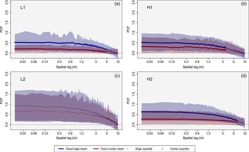
7298                                     D. S. Dodson and J. D. Small Griswold: Droplet Inhomogeneity in Shallow Cumuli

bution, while most observed distributions are much broader.          bulent air, with a decrease in the observed inhomogeneity
For example, the predicted growth time of precipitation cal-         in time due to turbulent mixing. Large-scale spatial inhomo-
culated by Jonas (1996) of 80 min is 4 times slower than that        geneities resulting from mixing have also been observed and
observed. Although progress in modeling the formation of             discussed by Saw et al. (2008, 2012).
rain has been made (i.e., Wyszogrodzki et al., 2013; Seifert            Up until the late 1980s, it was mostly accepted that droplet
et al., 2010; van Zanten et al., 2011), improvements still           spacing within clouds was statistically homogeneous, or uni-
need to be implemented – in particular, in developing a bet-         formly distributed according to Poisson statistics (Marshak
ter understanding of precipitating processes and the resulting       et al., 2005; Rogers and Yau, 1989). Srivastava (1989) ar-
feedbacks to implement better microphysical schemes (Wys-            gued that in most numerical studies of cloud physics it is
zogrodzki et al., 2013). It has long been proposed that the en-      assumed that droplet-to-droplet variability is not important
trainment of dry air into the cloud causes the broad size dis-       in calculating the growth of an ensemble of droplets. How-
tributions observed (Warner, 1969; Telford and Chai, 1980;           ever, this conclusion must be viewed as tentative due to ev-
Jonas and Mason, 1982). Khain et al. (2000) states that the          idence that has been gathered over the past three decades
smallest droplets form through nucleation of drops during            for the inhomogeneous distribution of droplet populations at
entrainment of drop-free air into the cloud, while the largest       all length scales (i.e., Baker, 1992; Kostinski and Jameson,
droplets are formed during inhomogeneous mixing leading              1997; Kostinski and Shaw, 2001; Larsen, 2007; Shaw et al.,
to a local increase in the supersaturation.                          1998, 2002; Saw et al., 2008, 2012; Good et al., 2012). The
   Enhanced evaporation from smaller droplet sizes arises            presumption that droplet spacing is homogenous has conse-
from aerosol perturbations, resulting in a stronger horizontal       quences for cloud parameterizations in microphysical mod-
buoyancy gradient and increased entrainment (known as the            els such as the formation of precipitation. For example, the
evaporation–entrainment feedback mechanism), as shown in             stochastic collection equation, used to describe the growth
both simulation (Xue and Feingold, 2006) and observational           of droplets via collision–coalescence, assumes that droplets
(Small et al., 2009) studies, where increased (decreased) en-        are homogeneously distributed and not preferentially con-
trainment leads to decreased (increased) cloud lifetimes. This       centrated (Kostinski and Shaw, 2001). An enhanced collision
suggests that aerosol perturbations can lead to modifications        kernel and collision efficiency also results from droplet clus-
in the turbulent environment within clouds, specifically at the      tering (Pinsky et al., 1999; Grabowski and Wang, 2013).
entrainment interface, influencing the amount of dry air be-            Analyses of droplet observations in adiabatic cores of cu-
ing entrained into the cloud.                                        mulus clouds from Chaumat and Brenguier (2001) display
   It is generally assumed that sub-saturated (droplet-free and      droplets that are randomly distributed (homogeneous) on the
laminar) ambient air is entrained in “blobs” due to the turbu-       small and large scales, albeit this homogeneous droplet dis-
lent motions of the cloud. This results in a reduction in the        tribution is observed in adiabatic cores away from dry air
total liquid water and directly influences the droplet size dis-     entrainment at cloud edge. These results are in disagreement
tribution. As suggested by Baker et al. (1980), the exact in-        with the aforementioned studies in the previous paragraph,
fluence of entrainment mixing on the drop size distribution          suggesting more in situ studies into droplet spatial inhomo-
can be described by the Damköhler number (see Small et al.,          geneity need to be performed. The in situ observations of
2013), which relates the timescales for turbulent mixing             droplet spatial distributions that do exist are scarce, with
(τmix ) and droplet evaporation(τevap ). Homogeneous mixing          most studies (i.e., Shaw et al., 2002; Lehmann et al., 2007)
(τevap  τmix ) results in the drop size distribution shifting to-   focusing on single cloud traverses and/or quantifying the sta-
wards smaller diameters due to all droplets experiencing the         tistical tools used to measure said inhomogeneity. Our un-
same sub-saturation. Inhomogeneous mixing (τevap  τmix )            derstanding of the motion of inertial particles in turbulence
results in a decrease in the overall droplet number (while           has advanced considerably, particularly due to the study of
the drop size distribution remains unshifted) due to droplets        inertial clustering at the Kolmogorov scales (i.e., Maxey,
experiencing different sub-saturated and super-saturated val-        1987; Squires and Eaton, 1991; Shaw et al., 1998; Eaton
ues.                                                                 and Fessler, 1994; Sundaram and Collins, 1997). However,
   After initial entrainment of the ambient, drop-free air into      this understanding has not been extended to particles being
the cloud, the subsequent turbulent mixing within the cloud          clustered due to larger-scale influences such as the entrain-
acts to produce smaller and smaller parcels of sub-saturated         ment mixing found at the boundaries of clouds. The work
cloudy and ambient air until the Kolmogorov length scale             conducted here therefore becomes important due to the fact
(approximately 1 mm for atmospheric conditions, depending            that a data set is provided that gives in situ cloud droplet spa-
on the turbulent kinetic energy dissipation rate) is reached         tial data allowing for an investigation into the influence that
(Baker et al., 1984; Brenguier, 1993). Direct numerical sim-         entrainment has on the droplet spatial distribution.
ulations by Ireland and Collins (2012) and experimental re-             Specific questions in regards to droplet inhomogeneity in
sults by Good et al. (2012) of particle entrainment showed           shallow, warm continental cumulus clouds to be answered in-
droplet inhomogeneity resulting from the initial entrainment         clude the following. (1) Does droplet inhomogeneity change
of particle-free (non-turbulent) air into the particle-laden tur-    as a function of location (cloud center vs. edge)? It is hypoth-

Atmos. Chem. Phys., 19, 7297–7317, 2019                                               www.atmos-chem-phys.net/19/7297/2019/
D. S. Dodson and J. D. Small Griswold: Droplet Inhomogeneity in Shallow Cumuli                                              7299

esized that said inhomogeneities will be enhanced at cloud         where ρa and ρw represent the density of air and liq-
edge where entrainment of dry air is directly occurring. Tur-      uid droplets, respectively; d the droplet diameter; ν the
bulent mixing will reduce the large-scale inhomogeneities in       fluid kinematic viscosity; ε the turbulent energy dissipation
the droplet population moving towards cloud center. (2) Does       rate; τd the particle response time; and τK the Kolmogorov
droplet inhomogeneity change as a function of cloud height?        timescale. The Stokes number characterizes a particle’s in-
It is hypothesized that an increase in inhomogeneity will be       ertial response to the flow. Particles with St  1 react very
present near cloud top due to the entrainment of dry air.          slowly to changes in the flow, while particles with St  1
(3) Does droplet inhomogeneity depend on aerosol number            follow the flow exactly. For the range of Stokes number in
concentration? It is hypothesized that an increased aerosol        clouds (St  1 to St < 1), inertial clustering increases as the
load leads to enhanced inhomogeneities due to the resulting        droplet size increases or as the turbulent dissipation rate in-
increased entrainment from smaller droplet sizes and evapo-        creases, with inertial clustering peaking at St ∼ 1 and de-
ration.                                                            creasing for smaller Stokes values.
   This is a first step in developing a better understanding of       However, the mechanism responsible for inertial cluster-
droplet inhomogeneities as a result of entrainment mixing, in      ing is completely unrelated to droplet inhomogeneities that
the hopes of eventually leading to better cloud microphysical      result from entrainment mixing, which is the focus of the
parameterizations for modeling precipitation and the overall       work presented here. Inhomogeneous mixing (i.e., entrain-
role of clouds in radiation models. Section 2 will provide a       ment mixing) leads to the mixing of particles from one re-
deeper introduction into droplet inhomogeneity along with          gion of the flow to another on a spatial scale comparable
the pair-correlation function (the statistical tool used to mea-   to the length scale of the mixing eddies. The largest eddies
sure the magnitude of droplet inhomogeneities). Section 3          are slightly smaller than the length scale of the cloud itself
will discuss data collection and instrumentation along with        (Grabowski and Clark, 1993), while the smallest mixing ed-
environmental and flight characteristics. Results related to       dies are on centimeter scales. These mixing length scales
the three scientific questions proposed above are presented        have been observed in non-precipitating continental cumu-
in Sect. 4. Finally, in Sect. 5 we discuss and summarize the       lus, with observations of the largest mixed cloud and clear
work presented and provide suggestions for extending the           air parcels on the scale of meters to tens of meters (Paluch
analysis presented here.                                           and Baumgardner, 1989), with the smallest parcels down to
                                                                   centimeter scales from turbulent mixing of the larger parcels.
                                                                   Other observations (Baker, 1992; Brenguier, 1993) suggest
                                                                   sharp interfaces between mixed parcels down to centimeter
2     Droplet inhomogeneity and the pair-correlation
                                                                   scales, with Brenguier (1993) observing a change from near 0
      function (PCF)
                                                                   to 2000 drops per cubic centimeter over a length scale of ap-
                                                                   proximately 5 mm. These observations support the concep-
2.1    Droplet inhomogeneity
                                                                   tual ideas of entrainment mixing, with the initial engulfment
                                                                   of ambient air followed by turbulent mixing of cloudy air
As briefly introduced in Sect. 1, droplet inhomogeneity in-
                                                                   down to the smallest scales.
herently occurs on different spatial scales. It has been pro-
                                                                      Entrainment is found to be governed by the large-scale
posed in multiple studies (i.e., Shaw et al., 1998; Eaton and
                                                                   parameters of the flow. Veeravalli and Warhaft (1989) and
Fessler, 1994; Sundaram and Collins, 1997) that inertial clus-
                                                                   Kang and Meneveau (2008) show that the entrainment inter-
tering can be understood as the result of particles being cen-
                                                                   face is characteristic of turbulent bursts penetrating the low-
trifuged out of regions of high fluid vorticity (where vorticity
                                                                   turbulence region, resulting in non-turbulent (drop-free) air
is a measure of local rotation in a fluid flow) and thus prefer-
                                                                   being entrained into the turbulent region. The non-turbulent
entially concentrating into regions of high strain or low fluid
                                                                   air then becomes turbulent through the viscous diffusion of
vorticity as a consequence of their inertia. Sundaram and
                                                                   vorticity at the interface. The viscous diffusion of vortic-
Collins (1997) have shown that the scale most responsible
                                                                   ity is a Kolmogorov-length-scale process, while the entrain-
for preferential concentration is the Kolmogorov scale. This
                                                                   ment rate at large Reynolds numbers is known to be inde-
is partially supported by the fact that vorticity plays a key
                                                                   pendent of viscosity. This suggests that although the tran-
role in concentrating particles, and vorticity is predominantly
                                                                   sition from non-turbulent to turbulent occurs through small
concentrated in the smallest eddies (Tennekes and Lumley,
                                                                   eddies, its rate is governed by the larger eddies (Hunt et al.,
1972).
                                                                   2006). This suggests that the rate of entrainment determines
   Saw et al. (2008), Hogan and Cuzzi (2001), and Wood
                                                                   the magnitude of droplet inhomogeneity present, with more
et al. (2005) have shown that inertial clustering is very sensi-
                                                                   entrainment leading to larger droplet inhomogeneities due to
tive to the particle Stokes number, given by
                                                                   larger and more numerous packets of environmental air being
                     1
                                                                   mixed with the cloud.
       τd   ρw d 2 ε 2                                                Good et al. (2012) and Ireland and Collins (2012) have
St =      =         3
                       ,                                    (1)
       τK   18ρa ν 2                                               shown that mixing-driven droplet inhomogeneities are only

www.atmos-chem-phys.net/19/7297/2019/                                               Atmos. Chem. Phys., 19, 7297–7317, 2019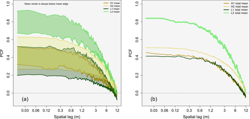
7300                                     D. S. Dodson and J. D. Small Griswold: Droplet Inhomogeneity in Shallow Cumuli

weakly dependent on the particle Stokes number. Unlike              where fk (t) is the probability distribution function that the
inertial clustering, large-scale droplet inhomogeneities due        kth particle posterior to a particle at to (the kth nearest neigh-
to entrainment should exist even as the Stokes number ap-           bor) is located at to + t, where it is assumed that co-located
proaches zero. Droplet inhomogeneity would only be re-              particles are impossible. Each of the fk (t) can be estimated
duced as the Stokes number approaches infinity (such as             from the observed inter-arrival distributions (time between
heavy particles) due to the droplets not following the turbu-       droplet arrival), thus allowing a computationally simple way
lent flow as dry air is entrained.                                  to compute the PCF from particle arrival times (Picinbono
   The effect that gravity (i.e., droplet sedimentation) has on     and Bendjaballah, 2005; Larsen, 2007, 2012).
the droplet response to the fluid must also be considered.             The main advantage of the PCF is the fact that it is scale
Grabowski and Vaillancourt (1999) suggest that if the droplet       localized. The PCF depends only on the presence or absence
terminal velocity is much larger than the Kolmogorov veloc-         of particles separated by t in time (Larsen, 2012). Physically,
ity scale, then the particle will fall through the microscale       when η(t) > 0 there is an enhanced probability of finding a
structures associated with the turbulent flow regardless of the     particle in the time frame t. The range of the PCF is (−1, ∞),
particle inertia. Ireland and Collins (2012) found that parti-      with η(t) = 0 representing perfect randomness and η(t) = 3,
cles are less dependent on the turbulent fluctuation for en-        for example, resulting in a factor of 4 enhancement of finding
hanced gravity, leading to lower levels of droplet inhomo-          another droplet time t away, as discussed in Kostinski and
geneity as compared to the reduced gravity case. Ireland and        Shaw (2001).
Collins (2012) also found enhanced settling of droplets with           When measuring data that are non-stationary (i.e., large-
moderate Stokes numbers (larger droplet size), consistent           scale spatial inhomogeneities are present), the PCF measures
with the findings in Wang and Maxey (1993) where droplets           droplet spatial heterogeneities that are a result of inertial
tended to cluster at the edges of vortical eddies leading to a      clustering and entrainment mixing (Saw et al., 2008, 2012).
preferential sweeping of the particles in a downward mov-           This results in a PCF (see Fig. 4 in Saw et al., 2012) with
ing fluid. On the other hand, Good et al. (2012) observed           a power-law-like region at the smallest scales (Kolmogorov
reduced settling for droplets with moderate Stokes numbers.         scales) due to inertial clustering, followed by an extended
This contradiction suggests more research into droplet spatial      “shoulder” region due to entrainment mixing at larger scales
tendencies is needed. It is also important to note that the stud-   (above Kolmogorov to tens of meters), followed by a rapid
ies just discussed present results for Reynolds numbers that        drop-off at even larger scales. Figure 3 in Shaw et al. (2002)
are smaller than those encountered in atmospheric clouds.           demonstrates two PCF plots, one with data from an entire
Although the Reynolds number is shown to have a very weak           cloud penetration and another with only cloud center data.
dependence (if any at all) on droplet inhomogeneities, the re-      The PCF for the entire cloud traverse is shown to be shifted
sults presented here can be used to compare in-cloud mea-           to larger clustering values due to large-scale droplet concen-
surements with measurements from laboratory experiments             tration fluctuations caused by “holes” in the cloud. Although
made by Ireland and Collins (2012) and Good et al. (2012).          Shaw et al. (2002) does not elaborate on the cause of these
                                                                    cloud holes, for our purposes we can think of them as areas
2.2    Pair-correlation function                                    of decreased droplet concentration due to the entrainment of
                                                                    dry environmental air into the cloud and subsequent filamen-
There are multiple tools that can be used to measure droplet        tation during turbulent mixing.
clustering using a time series of droplet detection times, but
the 1-D temporal pair-correlation function (PCF) will be used       2.3   Calculating the PCF
throughout this paper due to the advantages of the PCF out-
lined in Shaw et al. (2002), Shaw (2003), Larsen (2007,             The PCF was calculated three times for each cloud penetra-
2012), and Baker and Lawson (2010). The PCF can be intro-           tion (120 m section, representing roughly 2 s worth of data)
duced as a scale-localized deviation from a stationary Pois-        at cloud edge (cloud entry and exit) and cloud center. To
son distribution, where the PCF is given by                         calculate the kth nearest neighbor, a maximum time inter-
         p(to + t|to )                                              val (t-max) and time bin (dt) are selected. Careful consider-
η(t) =                 −1                                    (2)    ation must be given. Set dt too small, and the PCF will be
              λ
                                                                    too noisy. Set dt too large, and you end up doing unneces-
from Larsen (2012), where η(t) is the PCF, p(to + t|to ) is the     sary scale averaging which results in a poor estimate of the
probability of finding a particle in the time lag to + t given a    PCF. Typically, t-max is an order of magnitude or so above
particle detected at some time to , and λ is the mean number        the mean inter-arrival time (mean time between each droplet
of droplets per time bin. Calculating p(to + t|to ) can become      within the data) of the particles and sets the maximum tem-
simplified by using                                                 poral lag. A dt of 0.0003 s and a t-max of 0.2 s were selected
                  ∞
                                                                    for all PCF calculations throughout this paper. This results in
               1X                                                   a vector ranging from 0 to 0.2 by 0.0003, giving the tempo-
η(t) = −1 +          fk (t),                                 (3)
               λ k=1                                                ral lag (x axis) for each PCF measurement. This results in a

Atmos. Chem. Phys., 19, 7297–7317, 2019                                               www.atmos-chem-phys.net/19/7297/2019/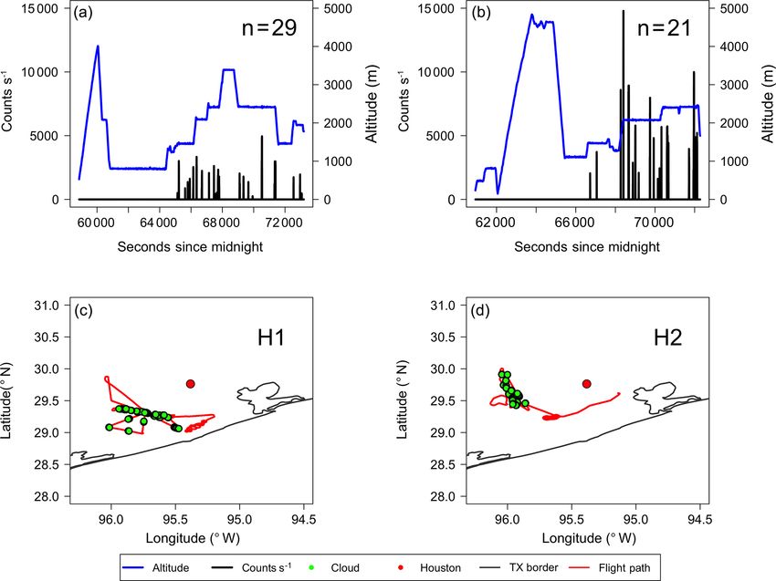
D. S. Dodson and J. D. Small Griswold: Droplet Inhomogeneity in Shallow Cumuli                                                     7301

spatial range of ∼ 3 cm to 12 m, which is ideal for analyzing     Table 1. Shows the flight information for 20 of the 22 flights that
droplet inhomogeneities due to entrainment mixing.                occurred during the GoMACCS campaign. Each flight corresponds
   The PCF is calculated by binning the inter-arrival times of    to a RF number, date, the number of clouds (after filtering; see text),
the droplets into the vector sequence discussed in the previ-     the total aerosol number concentration (Na ), and the accumulation
ous paragraph. An inter-arrival time is first determined be-      mode aerosol number concentration (Nacc ). Values in parentheses
                                                                  represent the standard deviation.
tween every subsequent droplet, binned and summed (the
sum of each inter-arrival time per bin). An inter-arrival
                                                                    RF number             Date   Clouds       Na cm−3      Nacc cm−3
time is then determined for every other droplet, every third
droplet, every fourth droplet, and so on. The inter-arrival         1                 8/21/06        1              n/a           n/a
times are binned and added to the previously summed binned          2                 8/22/06       11              n/a           n/a
inter-arrival times up until the minimum inter-arrival time         3                 8/23/06        9       2984 (588)      413 (66)
                                                                    4                 8/25/06       17    22667 (10672)   1797 (4184)
in the data is no longer less than t-max. The total summed          5                 8/26/06       18       1304 (699)     290 (223)
binned data are then used to calculate the PCF from Eq. (3).        6                 8/27/06        0              n/a           n/a
   Figure 1 gives a visualization and description of the PCF        7                 8/28/06        0              n/a           n/a
clustering signature, giving both temporal and spatial lag on       9                 8/29/06       28      3157 (1980)     360 (169)
the x axis. Note that the PCF results presented from this point     11                8/31/06       37       3205 (650)     972 (214)
on will be in spatial lag (where spatial lag was estimated us-      12                 9/2/06       29      4768 (2826)     710 (169)
                                                                    13                 9/3/06        0              n/a           n/a
ing the mean aircraft velocity) for the simplicity of being
                                                                    14                 9/4/06       14       2770 (758)     697 (126)
able to more easily comprehend spatial lag over temporal            15                 9/6/06       10       1427 (398)     465 (147)
lag. Real data (Fig. 1a) from a randomly selected cloud show        16                 9/7/06       32       3547 (966)     949 (306)
a peak in the PCF at smaller spatial scales and a decrease          17                 9/8/06       21      4824 (1806)     821 (154)
to zero at larger spatial scales (where the decrease starts at      18                9/10/06        1       1396 (918)     943 (472)
∼ 1.2 m), while simulated Poisson data (Fig. 1b) show the           19                9/11/06       27      6561 (5419)   1280 (4172)
PCF varying around zero, indicating no inhomogeneities at           20                9/13/06        0              n/a           n/a
                                                                    21                9/14/06       25      2230 (1157)     653 (276)
any scale. The PCF signature for the real data is indicative
                                                                    22                9/15/06       13       2323 (688)     436 (159)
of droplet inhomogeneity at larger scales, where the shoul-
der region of the curve is present before a decrease to zero      n/a – not applicable.
(note that inertial clustering is not presented since the curve
does not extend into small enough length scales). In com-
paring the two PCF curves, it is clear that the real cloud        to allow detailed sampling at different altitudes. The other 13
droplets have a greater amount of spatial inhomogeneity as        cases involved scattered cumuli that were sampled in such a
compared to droplets that have a perfectly random orienta-        manner as to provide statistical properties over the cloud field
tion, i.e., the simulated Poisson data. A better visual repre-    (Lu et al., 2008), with each cloud being traversed through
sentation of the droplet inhomogeneity that the PCF is dis-       once and no one cloud being measured multiple times.
playing can be gained by analyzing the raw droplets (Fig. 1c         Table 1 shows each flight conducted during GoMACCS,
and d), where the real data are patchy or clustered and the       with the corresponding research flight (RF) number, date,
Poisson point data are nearly perfectly homogeneous.              number of clouds in the flight after filtering (including clouds
                                                                  that are only > 300 m in length and non-precipitating), the
                                                                  aerosol number concentration (Na , measured by the conden-
3   Data collection and characteristics                           sation particle counter, CPC), and the aerosol number con-
                                                                  centration for accumulation mode particles (Nacc , measured
The Gulf of Mexico Atmospheric Composition and Cli-               by the passive cavity aerosol spectrometer probe, PCASP),
mate Study (GoMACCS) was conducted jointly with the               which includes aerosols that are only in the size range of
2006 Texas Air Quality Study (TexAQS) during August and           0.1 µm < particle size < 2.5 µm. The phase-Doppler interfer-
September of 2006 as a combined climate change and air            ometer (PDI; see Chuang et al., 2008) was used to collect
quality intensive field campaign. The Center for Interdisci-      droplet velocity, size, and measurement time. It was found
plinary Remotely Piloted Aircraft Studies (CIRPAS) Twin           that the droplet arrival time can accurately be measured to
Otter aircraft (flight speed of about 60 m s−1 ) performed 22     < 3.5 µs from Saw (2008), resulting in accurately mapping
research flights to explore aerosol–cloud relationships over      droplets down to 2.1 × 10⁻⁴ m (assuming average aircraft
the Houston and northwestern Gulf of Mexico regions (Lu           speed). Note that there is no dead time in PDI measurements.
et al., 2008). Among the 22 research flights, 14 intensive        For more information on each of the flights and the instru-
cloud measurements were carried out (where the clouds were        ment payload, see Lu et al. (2008).
all continental warm cumulus subjected to various levels of          Following the methods in Small et al. (2013), two low
anthropogenic influence), including one flight in which an        (L1 and L2, where L1 (L2) is given by RF 5 (RF 22)) and
isolated cumulus cloud of sufficient size and lifetime existed    high (H1 and H2, where H1 (H2) is given by RF 12 (RF

www.atmos-chem-phys.net/19/7297/2019/                                                     Atmos. Chem. Phys., 19, 7297–7317, 2019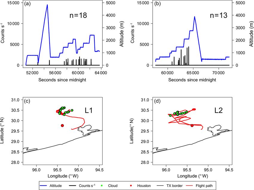
7302                                       D. S. Dodson and J. D. Small Griswold: Droplet Inhomogeneity in Shallow Cumuli

Figure 1. Panels (a) and (b) represent the clustering signature for the PCF, with the x axis showing the temporal and spatial lag on a log
scale and the y axis representing the PCF (unitless). Panel (a) shows the PCF for data from a randomly selected portion of cloud covering
a temporal range of 2 seconds (∼ 120 m) with a population of 2168 droplets. Panel (b) shows simulated Poisson point data with the same
temporal scale and droplet population. The red line represents a rolling mean of five for the raw PCF values (shown in black). Panels (c)
and (d) represent short 25 m subsets (∼ 270 droplets) of the data used in generating the PCF curves. Each circle represents a cloud droplet,
and each line with vertical bars represents the distance traversed for each sampling volume, with each vertical bar corresponding to a droplet
count of 10. The green vertical line is used for reference, where the mean value of the PCF is obtained by taking PCF values to the left of the
green line.

18)) pollution flights were selected out of the 22 research               archived wind data from the NOAA National Centers for
flights. The two least and most polluted flights which had                Environmental Information and HYSPLIT trajectories (not
satisfactory cloud sampling were selected for analysis of how             shown here) from the Air Resources Laboratory (Stein et al.,
aerosol number concentration affects droplet inhomogeneity.               2015).
A case flight (RF 18) was selected where an isolated cu-                     It can be calculated from analyzing Table 3 that the high-
mulus cloud was sampled at different altitudes for analysis               pollution clouds had roughly 2.5 times more aerosols per cu-
of droplet inhomogeneity as a function of cloud height. Ta-               bic centimeter than the low-pollution clouds. The difference
ble 2 shows variables highlighting different cloud and envi-              in aerosol number concentration between the low- and high-
ronmental conditions within each flight. Note that the envi-              pollution clouds produces clouds that are statistically differ-
ronmental lapse rate and relative humidity (RH) in Table 2                ent from one another. Figure 4 shows cloud droplet diameter
was calculated from data collected from out-of-cloud spirals,             in microns (µm) on the x axis with aerosol number concen-
where the average RH was computed for the vertical range                  tration (cm−3 ) on the y axis, with low-pollution data in green
of cloud measurements for the respected flight. As a result of            and high-pollution data in gold. Density curves are given
RH measurement problems occurring throughout the cam-                     to show how the data are distributed for the respected axis.
paign (i.e., values considerably above 100 %) the RH data                 The p value (used to determine statistical significance be-
were filtered to include values that were only less than 103 %.           tween two data sets, where p value < 0.05 is considered sig-
Table 3 gives a summary of average values for low- and high-              nificant; see Wilks, 2011) between low- and high-pollution
pollution cases for select properties from Table 2.                       cloud droplet size is 3.99 × 10⁻¹⁰ (average droplet diameter
   Figures 2 and 3 show the flight altitude as a function of              is 13.4 µm (10.7 µm) for low (high) pollution clouds). The
time with droplet counts per second overlaid (panels a and b)             linear best-fit trend lines show that droplet size decreases
and the flight paths (panels c and d) for weakly and highly               with increasing aerosol number concentration, with R 2 val-
polluted clouds, respectively. Note that the flight path for              ues (the proportion of the variance in droplet size that is pre-
the case flight is not shown here. The average droplet counts             dictable from the aerosol number concentration) of 0.24 and
(clouds) encountered per second (flight) for L1 and L2 were               0.07 for low and high pollution, respectively. The p value
660 (18) and 1016 (13), respectively, whereas for H1 and H2,              for the aerosol number concentration is < 2.22×10⁻¹⁶ . Both
the average counts (clouds) encountered per second (flight)               properties of the droplet population have p values less than
were 958 (29) and 3300 (21), respectively. Low-pollution                  0.05, making the difference in droplet size and aerosol num-
clouds were sampled to the north of Houston (upwind) and                  ber concentration significant for the two populations of data.
high-pollution clouds were sampled to the southwest (H1)                  Having two statistically different data populations is ideal for
and west (H2) of Houston (downwind), as confirmed using                   comparing PCF values for low- and high-pollution clouds.

Atmos. Chem. Phys., 19, 7297–7317, 2019                                                      www.atmos-chem-phys.net/19/7297/2019/
D. S. Dodson and J. D. Small Griswold: Droplet Inhomogeneity in Shallow Cumuli                                                     7303

Table 2. A summary of cloud, flight, and environmental properties from the L1, L2, H1, H2, and case flights. Note that CDNC stands
for cloud droplet number concentration, LWC stands for liquid water content, and mean drops (s−1 ) represents the mean number of drops
measured by the PDI per second. Standard deviation values are represented in parentheses.

             Variable                                            L1            L2             H1             H2           Case
             Date                                     26 Aug 2006     15 Sep 2006     2 Sep 2006     6 Sep 2006    10 Sep 2006
             Flight number                                    RF 5          RF 22          RF 12          RF 17           RF 18
             UTC for cloud sampling                    1447–1717       1654–1748      1806–2018      1832–2002      1633–1742
             Clouds > 300 m in width                             18             13             29             21               1
             Min cloud base height (m)                         672           1120           1457           1476             806
             Max cloud top height (m)                         2412           2101           2463           2451            3381
             Cloud thickness (m)                              1740            981           1007            976            2575
             Cloud width (m)                             700 (235)      520 (110)      850 (404)      861 (451)       943 (472)
             Mean true air speed (m s−1 )                61.2 (1.5)     59.9 (1.3)     62.7 (2.3)      63.0(2.3)      61.4 (2.2)
             Mean CDNC (cm−3 )                           318 (163)      210 (141)      421 (255)       531(363)       472 (404)
             Max CDNC (cm−3 )                                  819            526           1059           1630            2342
             Mean drops (s−1 )                           661 (448)    1016 (1037)      958 (895)    3300 (2704)    1679 (1441)
             Cloud top LWC (g m−3 )                     0.97 (0.66)    0.55 (0.54)    0.47 (0.48)    0.60 (0.48)    0.45 (0.35))
             Mean vertical velocity (m s−1 )            1.81 (1.67)    1.16 (1.28)    2.34 (2.21)    1.61 (1.62)     0.35 (1.89)
             Na (cm−3 )                                 1304 (699)     2323 (688)    4768 (2826)    4824 (1806)      1396 (918)
             Nacc (cm−3 )                                290 (223)      436 (159)      710 (169)      821 (154)       943 (472)
             Environmental lapse rate (◦ C km−1 )               5.4            4.5            4.8            5.7             n/a
             Environmental RH (%)                                77             96             74             86             n/a

           n/a – not applicable.

Table 3. Average values for low (L1, L2) and high (H1, H2) pollu-         represent the 85th and 15th percent quantile of the data. The
tion clouds for select variables from Table 2.                            center lines in each envelope represent the edge and center
                                                                          mean inhomogeneity, with bold mean lines representing data
         Variable                         Low           High              that are statistically significant (p value less than 0.05) and
         Mean CDNC (cm−3 )                 264            476             thin mean lines representing data that are statistically simi-
         Mean drops (s−1 )                 839          2129              lar. The PCF functions for both center and edge data indicate
         Na (cm−3 )                      1814           4796              clustering associated with larger-scale inhomogeneity, with
         Nacc (cm−3 )                      363            766             the shoulder region of the curves present out to ∼ 1.2 m be-
         Cloud thickness (m)             1361             992             fore a decrease to zero at spatial scales beyond ∼ 1.2 m.
         Cloud width (m)                   610            856                The main takeaway from Fig. 5 is the larger degree of in-
         Clouds > 300 m in width     31 (total)     50 (total)            homogeneity for cloud edge as compared to the center zones
                                                                          for all four flights. Mean PCF and quantile values for edge
                                                                          and center data can be found in Table 4. The mean and quan-
If the magnitude of spatial inhomogeneity does not change                 tile values were calculated by taking the first 60 PCF values
between the two, then an argument cannot be made for the                  (taking PCF values to the left of the green reference line in
statistical similarities in the data sets as a possible reason.           Fig. 1), covering a spatial scale up to ∼ 1 m since it is the
Note that all p values in this paper were calculated using the            shoulder region of the PCF curve that we are interested in an-
Wilcoxon rank-sum test, which is used to determine a sta-                 alyzing. The percent of statistically significant data (for the
tistical difference in the medians of two data sets that have             first 60 PCF values) and the corresponding p values can be
different populations (Wilks, 2011).                                      found in Table 5. Note that to calculate the p value every
                                                                          PCF curve generated for the respective plot was grouped. A
                                                                          p value was then generated for each spatial lag on the x axis
4     Results                                                             by calculating the Wilcoxon rank-sum test between the two
                                                                          sets of data for the specific x-axis location.
4.1    Edge, center, and cloud top inhomogeneities                           From analyzing Fig. 5 and the corresponding tables, L1,
                                                                          H1, and H2 show PCF characteristics which are comparable
PCF functions for L1, L2, H1, and H2 are given in Fig. 5,                 to one another, including the following. (1) The mean PCF
moving from Fig. 5a to d, respectively, with blue (red) rep-              value for the edge data is always greater than the mean PCF
resenting cloud edge (cloud center) data. The two envelopes               value for the center data. (2) The 15th percent quantile value

www.atmos-chem-phys.net/19/7297/2019/                                                      Atmos. Chem. Phys., 19, 7297–7317, 2019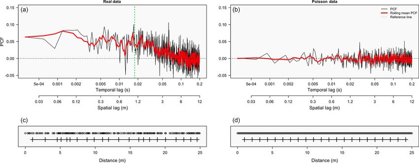
7304                                        D. S. Dodson and J. D. Small Griswold: Droplet Inhomogeneity in Shallow Cumuli

Figure 2. L1 and L2 are shown on the left and right, respectively. Flight altitude (blue) as a function of time is displayed in (a) and (b), with
droplet counts per second in black. The “n =” represents the number of clouds sampled for each flight after filtering. Panels (c) and (d) show
the Texas coast in grey with the location of Houston represented by the red dot. The flight path is outlined in red with the location of clouds
displayed by green dots.

Table 4. The mean PCF, 85th percent quantile, and 15th percent quantile values for center data (on the left) and edge data (on the right) for
L1, L2, H1, and H2 in Fig. 5, along with average low and high values from Fig. 9.

                                              Center data                                           Edge data
              Flight        Mean PCF      Upper quantile     Lower quantile      Mean PCF      Upper quantile     Lower quantile
              L1                  0.18               0.36               0.02           0.49               0.89               0.09
              L2                  0.61               1.39               0.16           0.83               1.62               0.14
              Avg. low            0.39               0.88               0.09           0.66               1.26               0.11
              H1                  0.26               0.69              0.009           0.46               0.86               0.09
              H2                  0.26               0.65               0.02           0.57               1.01               0.18
              Avg. high           0.27               0.67               0.01           0.52               0.93               0.14

for the center data is always smaller than the 15th percent                   From analyzing L2 (Fig. 5c) and the corresponding tables,
quantile value for the edge data. (3) The 85th percent quantile            there are significant differences from the other three cases.
value for the edge data is always larger than the 85th percent             Although the mean edge inhomogeneity is enhanced as com-
quantile value for the center data. (4) There is a statistical             pared to the center zone, the difference is not statistically sig-
significance between the inhomogeneities occurring between                 nificant, with 0 % of the data having a p value below 0.05
the edge and center zones of the clouds. Note that the sta-                (average p value of 0.40). Another difference is the range of
tistical significance in the inhomogeneities between the two               the quantile values, with the cloud edge data having a lower
zones breaks down at larger spatial scales (this is very appar-            15th percent quantile value than that of the center data, in
ent in the H1 case) as the PCF decays towards zero for both                contrast to what is observed in L1, H1, and H2. Note that the
entrainment and center data.

Atmos. Chem. Phys., 19, 7297–7317, 2019                                                       www.atmos-chem-phys.net/19/7297/2019/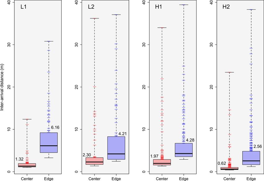
D. S. Dodson and J. D. Small Griswold: Droplet Inhomogeneity in Shallow Cumuli 7305
Figure 3. As in Fig. 2 but for H1 and H2.
Table 5. The mean p value and the percent of data that are statis-
tically significant (for the first 60 PCF values) between edge and
center data for L1, L2, H1, and H2 in Fig. 5 and for average low
and high in Fig. 9
Flight p value % significant
L1 5.9 × 10⁻³ 100
L2 0.40 0
Avg. low 0.01 100
H1 0.01 100
H2 3.5 × 10⁻⁴ 100
Avg. high 3.1 × 10⁻⁵ 100
mean inhomogeneity amount for L2 (both center and edge)
is enhanced as compared to the other three cases (Table 4).
It is clear that there are enhanced inhomogeneities in the
edge zone as compared to the center zone, but one needs
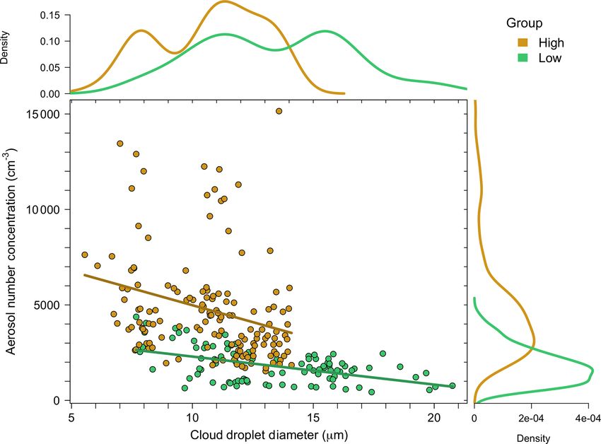
Figure 4. Shows cloud droplet diameter (µm) on the x axis and to understand how to define if the overall inhomogeneities
aerosol number concentration (cm−3 ) on the y axis, with low- (both edge and center) are significant as compared to a ran-
pollution data in green and high-pollution data in gold. The cor- domly distributed droplet population. This is done by ana-
responding density curves of the high- and low-pollution data are lyzing the range that the PCF can take on due to the ran-
given on the outer margins of the plot. dom nature of the data. If the physical inhomogeneities mea-
sured fall outside of this range, then the conclusion can be
made that the droplet spatial inhomogeneities being viewed
are indeed real and not perfectly homogeneous. This test was
www.atmos-chem-phys.net/19/7297/2019/ Atmos. Chem. Phys., 19, 7297–7317, 2019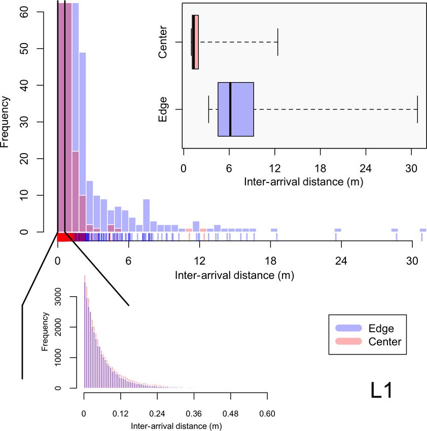
7306                                       D. S. Dodson and J. D. Small Griswold: Droplet Inhomogeneity in Shallow Cumuli

Figure 5. PCF clustering signatures for L1 (a), L2 (c), H1 (b), and H2 (d) with spatial lag (m) on the x axis and PCF values (unitless) on the
y axis. Edge data are in blue and cloud center data are in red, with the envelopes representing the 85th (a, b) and 15th (c, d) percent quantile
values of the data. The mean PCF value for each case is represented by the middle line in each envelope, where a bold mean line represents
edge and center differences that are statistically significant.

performed on each of the four cases, following the methods                Table 6. Percentage of inhomogeneities that are significant and non-
outlined in Larsen and Kostinski (2005). For the data, 1000               significant (as compared to a randomly distributed droplet popula-
Poisson simulations were produced (as is seen in Fig. 1b,                 tion) for center (C) and edge (E) data in L1, L2, H1, and H2.
showing a single Poisson simulation) using the same time du-
ration and droplet count as the original data. These Poisson                           Flight     % significant   % non-significant
simulations then form an envelope of PCF values (using the                             L1 C               44.4                 55.5
maximum and minimum values from the 1000 simulations)                                  L1 E               61.1                 38.9
one would consider homogeneous. PCF values that lie within                             L2 C               92.3                  7.7
the Poissonian simulation envelope were recorded by using                              L2 E               76.9                 23.1
the average PCF value and were labeled non-significant. Ta-                            H1 C               48.3                 51.7
ble 6 shows the percentage of PCF values for each flight and                           H1 E               58.6                 41.4
each location (edge and center) that were considered non-                              H2 C               71.4                 28.6
significant and significant. From analyzing Table 6 it can be                          H2 E               97.6                  2.4
seen that not every cloud section measured experienced in-
homogeneity that would be considered a statistical difference
from a random distribution. However, a majority of the data
sets do display inhomogeneities that are statistically signifi-           spatial distributions and the largest inhomogeneities mea-
cant, with the exception of the L1 center and H1 center data,             sured by directly analyzing the inter-arrival time distribution
which shows that less than 50 % of the droplet populations                (as is done in Baker, 1992). Figure 6 shows the inter-arrival
display statistically significant inhomogeneities. With the ex-           distance (IAD, distance between each droplet measurement)
ception of the L2 case (which does not have a statistical dif-            binned for L1 and zoomed in on a frequency of 60 as to put
ference between edge and center inhomogeneity), the center                more emphasis on the largest IADs measured. Zooming in
inhomogeneity contains a higher percentage of PCF values                  further on the first bin (range of 0 to 60 cm), where 98.4 %
that are non-significant as compared to the edge data.                    and 99.5 % of the data lie for edge and center data, respec-
   We can use the inter-arrival times used in calculating the             tively, it can be seen that the IADs follow a Poisson distri-
PCF to develop a better understanding of the overall droplet              bution. Analyzing the largest IADs, the box plot in the top
                                                                          left corner shows the data for center and edge that is greater

Atmos. Chem. Phys., 19, 7297–7317, 2019                                                         www.atmos-chem-phys.net/19/7297/2019/
D. S. Dodson and J. D. Small Griswold: Droplet Inhomogeneity in Shallow Cumuli 7307
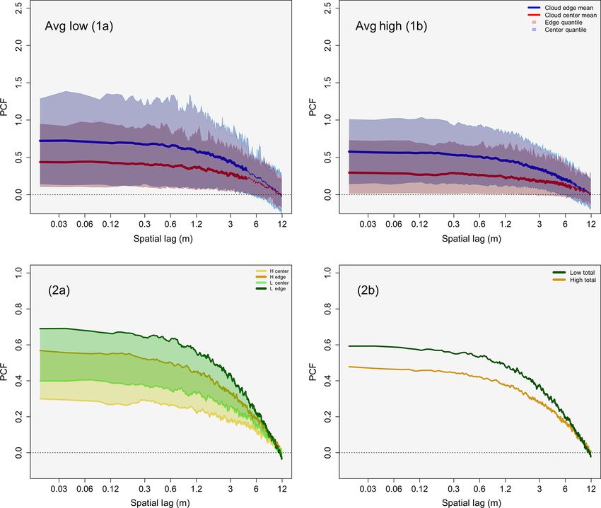
and other environmental properties (cloud droplet number
concentration, cm−3 ; liquid water content, g m−3 ; RH, %;
and vertical velocity, m s−1 ) vary with normalized cloud
height from the case flight. Variable quantities for each nor-
malized cloud height can be found in Table 7. The liquid wa-
ter content (LWC) increases from cloud base (0.073 g m−3 )
to a normalized cloud height of 0.7 (0.98 g m−3 ) before de-
creasing to 0.23 g m−3 at cloud top. Accompanied by the de-
crease in LWC is a sharp decrease in the RH from 91.8 %
to 38.4 % between normalized cloud heights of 0.7 and 0.9,
before increasing again at cloud top to 95.7 %. As both the
LWC and RH decrease, the PCF has a sharp increase from
0.36 to 1.49 between normalized cloud heights of 0.8 and 1.0,
indicating enhanced inhomogeneity at cloud top. The PCF
values at cloud top (between normalized cloud heights of 0.8
to 1.0) are statistically significant as compared to the PCF
values below a normalized altitude of 0.8 (with a p value of
0.043), making the inhomogeneity that is present at cloud top
statistically significant from the inhomogeneity that is occur-
ring in lower cloud layers.
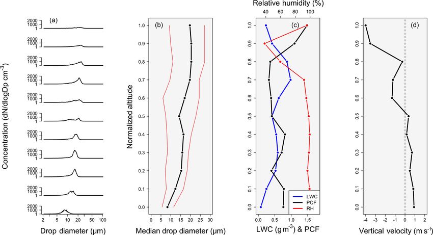
Figure 8a gives the cloud drop size distribution for each
Figure 6. Histogram distributions of the inter-arrival distance (IAD) normalized cloud height while Fig. 8b gives the median
for droplet populations measured in flight L1, with edge data in blue droplet diameter along with the 5th and 95th percent quan-
and center data in red. Note that the main histogram is zoomed in to tiles of the drop size distribution. The median drop size in-
a value of 60 on the y axis, with further analysis of the first bin (rep- creases from 8.29 µm at cloud base to 19.67 µm at cloud top.
resenting a range from 0 to 0.60 m) below the main histogram. The In comparing the median drop size to the mean PCF value
box plots in the top right represents the IAD data that are greater for each normalized height, the R 2 value is 0.041, indicat-
than or equal to the 0.998 quantile of the overall data sets for en- ing no correlation between the PCF and median droplet size.
trainment and center. Particulary at cloud top where the PCF increases, there is no
associated changes in the median drop size or the quantile
values of the size distribution. Figure 8d shows that the ver-
than or equal to the 0.998 quantile of the IAD data, i.e., the tical velocity is negative in the upper portion of the cloud,
largest 0.2 % of the IAD data. This results in approximately while an updraft is present in the lower 50 % of the cloud.
the largest 100 IADs to be represented in the box plot.
Although the raw histograms of IAD data are not dis- 4.2 Low- vs. high-pollution inhomogeneity
played for L2, H1, and H2 (they appear very similar in nature
to that of L1), the resulting box plots of the IAD data which Figure 9 panels (1a) and (1b) give the same information as in
are greater than or equal to the 0.998 quantile for each of Fig. 5, except for the PCF values for total low pollution (av-
the four flights are presented in Fig. 7, where the tick marks erage of L1 and L2) and total high pollution (average of H1
occurring on the upper whiskers represent the raw data posi- and H2), respectively. The characteristics of the two cluster-
tions for a better visualization of how the data are distributed. ing signatures are similar to that of Fig. 5. The average PCF
For each of the four flights, the edge data are shifted to larger values for low- and high-pollution edge and center data can
IAD values as compared to the center data, with the IADs be found in Table 4, along with the 15th and 85th percent
between the edge and center data being statistically signifi- quantile values. Table 4 reveals that the mean PCF values
cant for each of the four cases. Note that the median value (for both edge and center data) for the low-pollution case are
for each data set is displayed within the box plot. This tells larger than the corresponding mean PCF values for the high-
us that there are more numerous, larger pockets of droplet- pollution case. As can be seen in Table 5, 100 % of the first
free air within the edge zone as compared to the center zone. 60 spatial lags are statistically significant for both average
For example, in analyzing the box plots for L2, we can see low- and high-pollution cases between the edge and center
that there are five cases where there is a distance of 20 m or data.
greater between droplet measurements for the edge zone, as The larger mean inhomogeneity amount for the low-
compared to only one case for the cloud center zone. pollution clouds can be seen well in Fig. 9 panel (2a), which
Figure 8 shows how the mean PCF value (where, again, the shows low-pollution data in green and high-pollution data in
mean PCF value is obtained by taking the mean of all individ- gold. The boundaries of each green and gold envelope are
ual PCF values to the left of the green reference line in Fig. 1) created by the mean center (bottom of each envelope) and
www.atmos-chem-phys.net/19/7297/2019/ Atmos. Chem. Phys., 19, 7297–7317, 20197308 D. S. Dodson and J. D. Small Griswold: Droplet Inhomogeneity in Shallow Cumuli Figure 7. Box plots for the IAD data which are greater than or equal to the 0.998 quantile of the overall data sets for edge (blue) and center (red), with L1, L2, H1, and H2 shown moving from left to right, respectively. The median value for each data set is displayed within the plot. Tick marks occurring on the upper whiskers represent the raw data positions. Note that panel L1 represents the same box plot displayed in Fig. 6. Figure 8. Shows the cloud droplet size distribution in panel (a). Panel (b) gives the median droplet size along with the 5th and 95th percent quantiles (red) of the droplet size distribution. Panel (c) shows LWC (blue), RH (red), and the mean PCF value (black). Panel (c) shows vertical velocity. All variables are represented as a function of cloud normalized altitude. Atmos. Chem. Phys., 19, 7297–7317, 2019 www.atmos-chem-phys.net/19/7297/2019/
D. S. Dodson and J. D. Small Griswold: Droplet Inhomogeneity in Shallow Cumuli                                                       7309

Table 7. Values for vertical velocity (m s−1 ), RH (%), LWC (g m−3 ), the PCF, and the median drop size (µm), respectively, for each
normalized cloud height in Fig. 8.

                               Normalized     Vertical velocity     RH        LWC      PCF     Median drop
                               height                  (m s−1 )     (%)    (g m−3 )              size (µm)
                               0                          0.91    100.38       0.07    0.76            8.29
                               0.1                        0.84     99.28       0.24    0.77           12.32
                               0.2                        0.49     96.46       0.52    0.40           15.29
                               0.3                        0.71     98.46       0.59    0.71           15.85
                               0.4                        0.16     99.43       0.54    0.81           16.43
                               0.5                        0.36     98.19       0.41    0.41           14.23
                               0.6                       -1.31     94.91       0.62    0.39           17.03
                               0.7                       -1.22     91.83       0.98    0.32           19.67
                               0.8                       -0.28     59.72       0.87    0.36           20.39
                               0.9                       -3.52     38.43       0.41    1.10           20.37
                               1                         -4.00     95.72       0.22    1.49           19.67

Figure 9. Panels (1a) and (1b): as in Fig. 5, except for average low-pollution PCF values (L1, L2) in panel (1a) and average high-pollution
PCF values (H1, H2) in panel (1b). Panels (2a) and (2b): low-pollution data in green and high-pollution data in gold. Panel (2a) shows
envelopes that span the mean center PCF value (lower limit of the envelopes) to the mean edge PCF value (upper limit of the envelopes).
Panel (2b) gives the overall mean PCF for low- and high-pollution clouds.

edge (top of each envelope) inhomogeneity. Low-pollution                mean PCF value for high-pollution clouds is 0.43. Although
clouds are clearly offset to a higher inhomogeneity amount              it appears that low-pollution clouds experience more inho-
for both mean center and edge inhomogeneity. Figure 9 panel             mogeneity as compared to high-pollution clouds, the differ-
(2b) shows the overall mean of all the PCF values for low-              ence is statistically similar. The average p value is 0.19 for
and high-pollution clouds. The overall mean PCF value for               the first 60 spatial lags, with 0 % of the data being statistically
low-pollution clouds (average of entrainment and center in-             significant.
homogeneity for both L1 and L2) is 0.54, while the overall

www.atmos-chem-phys.net/19/7297/2019/                                                     Atmos. Chem. Phys., 19, 7297–7317, 2019
7310 D. S. Dodson and J. D. Small Griswold: Droplet Inhomogeneity in Shallow Cumuli
Table 8. The mean p value and the percent of data that are statisti- son (1984) found that the LWC decreases due to entrainment
cally significant (for the first 60 PCF values) between PCF functions as cumulus clouds deteriorate. Lu et al. (2013) and Cheng
provided in Fig. 10b. et al. (2015) also found that enhanced entrainment leads to
decreases in cloud droplet concentration, droplet size, and
Comparison p value % significant LWC.
L2–L1 2.2 × 10⁻³ 100 Figure 11 shows box plots of vertical velocity, LWC, cloud
L2–H1 1.3 × 10⁻³ 100 width, CDNC, buoyancy, and RH. Red median lines repre-
L2–H2 2.2 × 10⁻² 100 sent data sets that are statistically different when compared
L1–H1 0.86 0 to L2. Note that, except for cloud width, each variable is rep-
L1–H2 0.21 0 resented from 1 Hz data collected during in-cloud sampling.
H1–H2 0.19 0 From analyzing Fig. 11 (exact median values for variables
can be found in Table 9), L2 has the lowest median verti-
cal velocity, LWC, cloud width, and CDNC, with L2 being
Low-pollution clouds have a non-statistically significant statistically significant (p values found in Table 10) when
higher amount of inhomogeneity than high-pollution clouds, compared to the other three flights. The fact that L2 has the
with further analysis showing that the higher amount of inho- lowest median vertical velocity reflects the fact that clouds
mogeneity in the low-pollution case is due entirely to the L2 have smaller positive vertical velocities than those measured
flight. Figure 10 gives the same information as panels (2a) in the other three flights, suggesting weaker growth poten-
and (2b) in Fig. 9, except for the individual flights (L1, L2, tial. The low LWC in L2 signifies that entrainment of dry air
H1, H2) shown. From analyzing Fig. 10a, one can see the has been occurring, resulting in the evaporation of liquid wa-
mean center and edge inhomogeneity for L2 (light green en- ter droplets, reducing the LWC and the CDNC (Pruppacher
velope) is beyond the range of the other three flights. The and Klett, 1997). Although Schmeissner et al. (2015) does
total mean PCF for the clouds in L1, L2, H1, and H2 is not discuss cloud width, clouds that are dissipating would be
shown in Fig. 10b. L2 has a mean PCF value of 0.76, which is expected to have a smaller horizontal extent due to entrain-
roughly twice the mean PCF values (and statistically signif- ment of dry air leading to evaporation of cloud edge droplets
icant; see Table 8) of the other three flights, where L1 (dark as compared to mature clouds.
green), H1 (dark gold), and H2 (light gold) have mean PCF Figure 11f gives a box plot of in-cloud RH, with L2 having
values of 0.39, 0.40, and 0.46, respectively. The question the second-lowest in-cloud RH, while being statistically sim-
of whether inhomogeneity depends on aerosol number con- ilar to that of the other three flights. The red dots represent
centration cannot confidently be answered. Although Fig. 9 the median out-of-cloud RH (100 m before and after cloud
shows that low-pollution clouds have a larger amount of in- edge). L2 is the only flight where the RH increases out of the
homogeneity, statistically speaking the inhomogeneity be- cloud. The fact that the RH is larger, on average, outside of
tween low- and high-pollution clouds is the same. Further the clouds in L2 as compared to inside of the clouds could be
analysis shows that L1, H1, and H2 all have statistically sim- a sign of a large humid shell that is surrounding the individ-
ilar inhomogeneity values (see Table 8) with mean inhomo- ual clouds. The humid shell results from entrainment of dry
geneity amounts that are almost identical. Flight L2 has sta- air into the cloud while moist air is detrained out of the cloud
tistically significant inhomogeneity as compared to the other into the cloud-free environment, resulting in a lower (larger)
three cases and is solely responsible for causing the low- RH inside (outside) the cloud (Heus and Jonker, 2008; Jonker
pollution clouds to have a higher mean PCF value than that et al., 2008; Heus et al., 2008). More evidence for the large
of the high-pollution clouds. humid shell can be gathered from the vertical profiles of en-
vironmental RH reported in Table 2, where the average RH
(measured out of cloud) for the vertical range of cloud mea-
5 Discussion surements was 96.3 % for L2, while for the other flights the
RH was considerably lower.
5.1 Cloud lifetime hypothesis and inhomogeneity in L2 Figure 11e shows the in-cloud buoyancy, which was cal-
culated by taking the in-cloud and out-of-cloud (100 m be-
An explanation for the statistically different inhomogeneity fore and after cloud edge) virtual potential temperatures. L2
in L2 as compared to the other three cases could be cloud has the largest median buoyancy and is statistically signifi-
age. A study by Schmeissner et al. (2015) found that dissi- cant as compared to the other three flights. The clouds in the
pating clouds have five main characteristics, including a neg- L2 flight have five out of the six characteristics for decaying
ative buoyancy (m s−2 ) and vertical velocity, lower LWC and clouds, including the (1) lowest vertical velocity, (2) low-
cloud droplet number concentrations (CDNC) as compared est LWC, (3) lowest CDNC, (4) lowest cloud width, and
to actively growing clouds, and a larger RH shell around the (5) largest humid shell. The evidence points to the clouds in
cumulus cloud. Decaying clouds are also associated with the L2 decaying on average, therefore leading to larger droplet
enhanced entrainment of dry air, where Cooper and Law- inhomogeneities as more dry air is mixed into the clouds as
Atmos. Chem. Phys., 19, 7297–7317, 2019 www.atmos-chem-phys.net/19/7297/2019/You can also read