(LAPSE-RATE) Measurements from mobile surface vehicles during the Lower Atmospheric Profiling Studies at Elevation - a Remotely-piloted Aircraft ...
←
→
Page content transcription
If your browser does not render page correctly, please read the page content below
Earth Syst. Sci. Data, 13, 155–169, 2021
https://doi.org/10.5194/essd-13-155-2021
© Author(s) 2021. This work is distributed under
the Creative Commons Attribution 4.0 License.

        Measurements from mobile surface vehicles during the
         Lower Atmospheric Profiling Studies at Elevation –
            a Remotely-piloted Aircraft Team Experiment
                           (LAPSE-RATE)
        Gijs de Boer1,2 , Sean Waugh3 , Alexander Erwin4 , Steven Borenstein5 , Cory Dixon5,a , Wafa’a Shanti4 ,
                                         Adam Houston4 , and Brian Argrow5
              1 Cooperative  Institute for Research in Environmental Sciences, University of Colorado Boulder,
                                                    Boulder, Colorado, USA
                                2 NOAA Physical Sciences Laboratory, Boulder Colorado, USA
                           3 NOAA National Severe Storms Laboratory, Norman, Oklahoma, USA
                                  4 University of Nebraska – Lincoln, Lincoln, Nebraska, USA
             5 Integrated Remote and In Situ Sensing, University of Colorado Boulder, Boulder, Colorado, USA
                            a now at: Geotech Environmental Equipment, Denver, Colorado, USA

                               Correspondence: Gijs de Boer (gijs.deboer@colorado.edu)

                                  Received: 29 June 2020 – Discussion started: 24 August 2020
                     Revised: 4 November 2020 – Accepted: 25 November 2020 – Published: 28 January 2021

      Abstract. Between 14 and 20 July 2018, small unmanned aircraft systems (UASs) were deployed to the San
      Luis Valley of Colorado (USA) alongside surface-based remote sensors, in situ sensors, and radiosonde sys-
      tems as part of the Lower Atmospheric Profiling Studies at Elevation – a Remotely-piloted Aircraft Team Ex-
      periment (LAPSE-RATE). The measurements collected as part of LAPSE-RATE targeted quantities related to
      enhancing our understanding of boundary layer structure, cloud and aerosol properties and surface–atmosphere
      exchange and provide detailed information to support model evaluation and improvement work. Additionally,
      intensive intercomparison between the different unmanned aircraft platforms was completed. The current pa-
      per describes the observations obtained using three different types of surface-based mobile observing vehi-
      cles. These included the University of Colorado Mobile UAS Research Collaboratory (MURC), the National
      Oceanic and Atmospheric Administration National Severe Storms Laboratory Mobile Mesonet, and two Uni-
      versity of Nebraska Combined Mesonet and Tracker (CoMeT) vehicles. Over the 1-week campaign, a total
      of 143 h of data were collected using this combination of vehicles. The data from these coordinated activi-
      ties provide detailed perspectives on the spatial variability of atmospheric state parameters (air temperature,
      humidity, pressure, and wind) throughout the northern half of the San Luis Valley. These datasets have been
      checked for quality and published to the Zenodo data archive under a specific “community” setup for LAPSE-
      RATE (https://zenodo.org/communities/lapse-rate/, last access: 21 January 2021) and are accessible at no cost
      by all registered users. The primary dataset DOIs are https://doi.org/10.5281/zenodo.3814765 (CU MURC mea-
      surements; de Boer et al., 2020d), https://doi.org/10.5281/zenodo.3738175 (NSSL MM measurements; Waugh,
      2020), and https://doi.org/10.5281/zenodo.3838724 (UNL CoMeT measurements; Houston and Erwin, 2020).

Published by Copernicus Publications.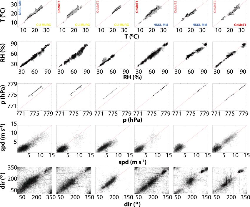
156                                       G. de Boer et al.: Measurements from mobile surface vehicles during LAPSE-RATE

1   Introduction                                                        During LAPSE-RATE, atmosphere-observing surface ve-
                                                                     hicles provided critical insight into gradients in state vari-
In July 2018, a collection of atmospheric scientists and en-         ables across the SLV, including information on temperature,
gineers from around the globe converged on the San Luis              pressure, humidity, and winds. This includes both single-
Valley (SLV) of Colorado (USA) to take part in the LAPSE-            site sampling and measurements covering extended transects
RATE (Lower Atmospheric Profiling Studies at Elevation –             conducted throughout the northern half of the SLV. The lat-
a Remotely-piloted Aircraft Team Experiment) field cam-              ter were particularly interesting given that the SLV features
paign (de Boer et al., 2020a, b). This campaign was focused          widely varying surface types (ranging from irrigated crop-
on demonstrating the utility of unmanned aircraft systems            land to dry shrublands), significant topography, and terrain-
(UASs) for atmospheric research and collecting scientifically        induced flows. The following section describes the vehicles
interesting datasets to conduct targeted studies on specific         deployed and instrumentation that they carried, while Sect. 3
topics of interest related to boundary layer processes. Con-         provides an overview of measurement locations and sam-
nected to the annual meeting of the International Society for        pling strategies. Section 4 provides details on data processing
Atmospheric Research using Remotely-piloted Aircraft (IS-            and quality control (QC), while Sect. 5 offers information on
ARRA, de Boer et al., 2019), LAPSE-RATE included over                dataset availability.
100 scientists and engineers, who together conducted nearly
1300 research flights and captured over 250 flight hours of          2     Instrument and vehicle descriptions
data using UASs.
   Information on the different UASs and profilers deployed          The three mobile surface-based platforms used to collect
during LAPSE-RATE, numerical simulations completed for               data during LAPSE-RATE and described in this paper in-
the campaign, and an overview of the campaign itself is dis-         clude the Mobile UAS Research Collaboratory (MURC), op-
tributed in a range of articles, many of which are associated        erated by the University of Colorado Boulder (CU), a mo-
with this Earth System Science Data special issue and will           bile mesonet (MM) vehicle operated by the NOAA National
not be revisited here (de Boer et al., 2020b, c; Bell et al.,        Severe Storms Laboratory (NSSL), and a pair of Combined
2020; Pillar-Little et al., 2020; Bailey et al., 2020; Natalie       Mesonet and Tracker (CoMeT) vehicles operated by the Uni-
et al., 2021; Islam et al., 2020; Brus et al., 2020; Pinto et al.,   versity of Nebraska Lincoln (UNL). As documented below,
2020). The current paper is focused on describing datasets           these three vehicles provided complementary measurements,
collected using mobile surface observing systems during the          including details on atmospheric temperature, pressure, hu-
LAPSE-RATE campaign.                                                 midity, and winds. Each operated in slightly different modes
   The general concept behind mobile surface-observing ve-           over the duration of the campaign, though all three vehicles
hicles is to provide a full mobile platform from which ac-           were at the same location for limited times.
curate observations of atmospheric parameters can be made,
thereby offering opportunities to position (and reposition) in
                                                                     2.1    CU MURC
situ surface meteorological instrumentation precisely to cap-
ture highly localized gradients and target locations that are        The CU MURC (Fig. 1) is an instrumented van that was
thought to be critical for the development of phenomena of           added to the Integrated Remote and In Situ Sensing (IRISS)
interest. To accomplish this, rack- or mast-mounted instru-          program vehicle fleet in early 2018. This system was specif-
mentation is set up to measure quantities such as pressure,          ically developed to work in tandem with unmanned aircraft
wind speed and direction, temperature, and relative humidity.        operations, serving as a mobile command station and surface
In the case of vehicles set up for truly mobile measurements         measurement facility during field deployments. This central-
(i.e., measuring while driving) instruments are mounted far          ized operations center provides a platform from which to
enough away from the vehicle structure to minimize direct            oversee field teams and provide general situational aware-
influence to the observations from the vehicle itself. Such          ness. The MURC is equipped with two workstations for
mobile mesonet systems have been deployed for atmospheric            lighter computing loads, including on-site processing of
research for over two decades, and details on the original mo-       data, real-time communications with team members and the
bile mesonets can be found in Straka et al. (1996). These            broader community through web-based systems, and possi-
systems have generally been used to evaluate atmospheric             bly serving as UAS ground stations. Additionally, the MURC
conditions supporting the development of tornadic supercells         carries two servers for more intensive computing tasks, with
(e.g., Markowski, 2002; Pietrycha and Rasmussen, 2004),              one dedicated to graphics-intensive processes (such as pro-
though deployments to observe land-falling hurricanes have           cessing of imagery for photogrammetry-centric missions)
also been conducted (e.g., Caban et al., 2019). Additionally,        and the other dedicated to general computing and intensive
mobile mesonet systems have been used in conjunction with            real-time data processing.
airborne systems (manned or unmanned) to capture measure-               From an observational perspective, the MURC is equipped
ments along four-dimensional transects (e.g., Riganti and            with a 15 m extendable mast, atop which are mounted sev-
Houston, 2017).                                                      eral meteorological sensors. This includes a Gill MetPak Pro

Earth Syst. Sci. Data, 13, 155–169, 2021                                              https://doi.org/10.5194/essd-13-155-2021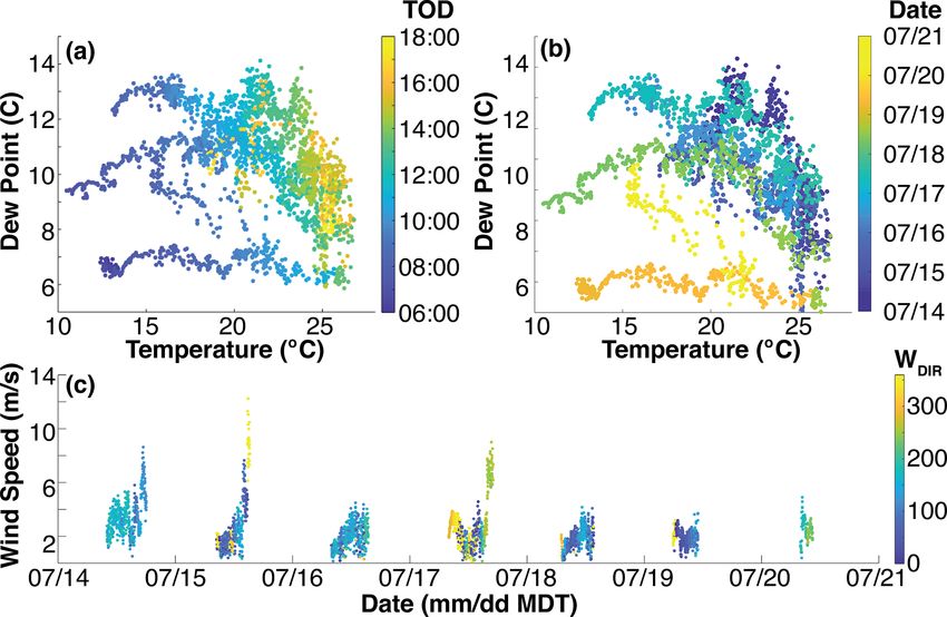
G. de Boer et al.: Measurements from mobile surface vehicles during LAPSE-RATE                                                      157

Figure 1. The CU MURC vehicle, with mast extended (a), as deployed during LAPSE-RATE. The right hand panels show the instrument
cluster mounted on the top of the MURC mast (b) and the MURC real-time data display (c).

Table 1. Sensor specifications for the CU MURC.

      Instrument name                              Observation             Range, accuracy              Response time
      Gill MetPak Pro                              Air temperature         −35– +70 ◦ C,                Not listed
                                                                           ∼ ± 0.1 ◦ C
                                                   Relative humidity       0 %–100 %,                   Not listed
                                                                           ± 0.8 % at 23 ◦ C
                                                   Barometric pressure     600–1100 hPa,                Not listed
                                                                           ± 0.5 hPa
                                                   Wind speed              0–60 m s−1 ,                 Not listed
                                                                           ± 2 % at 12 m s−1
                                                   Wind direction          0–359◦ ,                     Not listed
                                                                           ± 3◦ at 12 m s−1
      Gill WindMaster 3-D Sonic Anemometer         Wind speed              0–50 m s−1 ,                 Not listed
                                                                           < 1.5 % RMS at 12 m s−1
                                                   Wind direction          0–359◦ ,                     Not listed
                                                                           ± 2◦ at 12 m s−1
                                                   Sonic temperature       −40– +70 ◦ C,                Not listed
                                                                           < ± 0.5 % at 20 ◦ C
      R.M. Young Wind Monitor 05103                Wind speed              0–100 m s−1 ,                2.7 m [distance constant]
                                                                           ± 0.3 m s−1

Base Station that measures barometric pressure, air temper-            sensors and their projected accuracies is included in Table 1.
ature, and relative humidity; a Gill WindMaster 3-D sonic              The MURC is also equipped with a large communications
anemometer for 3-D wind and fast temperature measure-                  suite that increases the range of UHF/VHF vehicle-to-vehicle
ments; and an R.M. Young Wind Monitor (05103) propeller                radios used during field campaigns, increases cellular band-
and vane anemometer which provides a redundant horizontal              width for data transfer and communications, and improves
wind measurement and offers real-time situational awareness            the ground station to UAS communication link. While mo-
for nearby unmanned aircraft operators. An overview of the             bile, the MURC is set up to operate at a single location at any

https://doi.org/10.5194/essd-13-155-2021                                                   Earth Syst. Sci. Data, 13, 155–169, 2021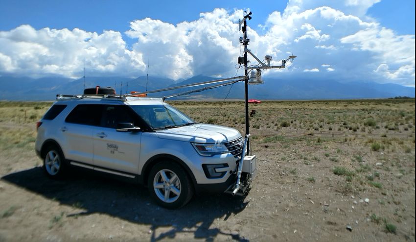
158                                          G. de Boer et al.: Measurements from mobile surface vehicles during LAPSE-RATE

Figure 2. The NSSL MM as deployed during the LAPSE-RATE project. The trailer is the University of Oklahoma CLAMPS system (see
Bell et al., 2020, in this special issue).

given time and does not collect measurements while travel-           this practice protects the RH observations from contami-
ing like other platforms described below. Data collected by          nation, it also significantly delays the thermal response of
the MURC were used to intercompare measurements from                 the environment inside the membrane. In combination with
the different UASs deployed during LAPSE-RATE. The re-               a relatively slow time constant (testing on previous models
sults of this intercomparison are documented in Barbieri et al.      such as the HMP35 and HMP45 have revealed time con-
(2019).                                                              stants on the order of 10 min; Waugh, 2012), the impacts
                                                                     of this membrane result in very slow response to tempera-
2.2   NSSL mobile mesonet                                            ture measurements (hence the designation “slow temp” for
                                                                     the HMP155). To overcome this, a fast-responding Camp-
In addition to the MURC, LAPSE-RATE included a deploy-               bell Scientific T109SS temperature sensor is also installed on
ment of the NOAA NSSL MM vehicle, a heavily modified                 the NSSL MM (T109, a.k.a. “fast temp”). The HMP155 can-
version of the original MM created 25 years ago (Straka              not be assumed to report a temperature and relative humidity
et al., 1996). The current generation of NSSL MM is built            that represents the true environmental conditions, only the
on a Ford F-250 extended-cab long-bed pickup truck. Instru-          conditions inside the membrane. However, while the HMP
mentation is located on a rack mounted forward and above             should not be used for temperature and relative humidity ob-
the hood of the vehicle, in order to minimize atmospheric            servations directly, dewpoint is conserved across the mem-
disturbances caused by the blunt forward edge of the truck           brane allowing the HMP to be useful for observing the dew-
(Fig. 2). Mounting the equipment rack over the roof of the           point (Richardson et al., 1998). This dewpoint observation is
vehicle (as was done with previous NSSL MM vehicles) was             combined with data from the faster T109 temperature sen-
thought to result in observational biases due to the turbu-          sor to derive a relative humidity value that is representative
lent and accelerated airflow over the vehicle roof and ther-         of the true environmental value (Richardson et al., 1998).
mal influence of the vehicle engine. The new setup requires          The thermodynamic observations are housed in a radiation
the addition of a substantial structure to support the weight        shield to protect the sensors from direct solar radiation while
and drag of the instrument rack. This structure also allows          maintaining adequate airflow from the real environment. This
for installation of a wire mesh hail cage to protect the wind-       shield, known as the “U-tube”, was developed by NSSL to
shield from hail strikes while operating in the vicinity of se-      specifically accomplish this task (Waugh and Frederickson,
vere thunderstorms. In addition to the instrument rack, the          2010; Houston et al., 2016). For wind measurements, the
MM can carry up to four helium tanks along with a Vaisala            NSSL MM deploys a standard propeller-vane combination
MW41 sounding system for mobile radiosonde launches.                 anemometer from R.M. Young (Wind Monitor 05103) cov-
   For air temperature and relative humidity measurements,           ering a wide range of wind speeds (0–100 m s−1 ). While the
the NSSL MM deploys a Vaisala HMP155 sensor. While                   vehicle is stationary, ambient wind direction is derived us-
the HMP155 is highly accurate, the relative humidity sen-            ing the vehicle-relative wind direction and vehicle heading
sor can be prone to contamination by atmospheric particles.          from a KVH C100 magnetic compass. In combination, these
To reduce this contamination the HMP155 requires integra-            allow for computation of the ambient wind vector. While in
tion of a membrane that allows water molecules to pass               motion, the vehicle-relative wind vector is subtracted from
through while reducing the impact of contaminants. While

Earth Syst. Sci. Data, 13, 155–169, 2021                                              https://doi.org/10.5194/essd-13-155-2021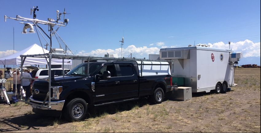
G. de Boer et al.: Measurements from mobile surface vehicles during LAPSE-RATE 159
Table 2. Sensor specifications for the NSSL MM and UNL CoMeT vehicles.
Instrument name Observation Range, accuracy Response time
Vaisala HMP155A Air temperature (slow) −80– +60 ◦ C, Not listed
∼ ± 0.1 ◦ C
Relative humidity 0 %–100 %, 63 % in 20 s
±1 %
Campbell Scientific T109SS Air temperature (fast) −40– +70 ◦ C, 7.5 s with 3 m s−1 flow
±0.6◦
R.M. Young Wind Monitor 05103 Wind speed 0–100 m s−1 , 2.7 m [distance constant]
±0.3 m s−1
Wind direction 0–360◦ , 1.3 m [distance constant]
±3◦
Vaisala PTB210 Barometric pressure 500–1100 mb, n/a
±0.15 mb
KVH C100 Fluxgate Magnetic heading 0–360◦ , n/a
±0.16◦
Garmin 19X HVS Lat./long./alt./heading/speed n/a n/a
n/a: not applicable
Figure 3. The UNL CoMeT vehicles, as deployed during LAPSE-RATE.
GPS-obtained vehicle motion to produce the inertial envi- ing a Vaisala HMP155A and also include a fast-response sen-
ronmental wind vector. The measurements from all of these sor (Campbell Scientific 109SS thermistor) for air tempera-
sensors are logged at 1 Hz using a Campbell Scientific CR6 ture at ∼ 2 m a.g.l. (same setup as the NOAA NSSL MM).
Wi-Fi-enabled data logger. A list of the sensors and their re- Air pressure at ∼ 2.5 m a.g.l. is measured using a Vaisala
spective measurements, as well as general accuracies and re- PTB210, while wind speed and direction are observed us-
sponse times are listed in Table 2. ing an R.M. Young 05103 propeller-vane anemometer at ap-
proximately 3.5 m a.g.l. The vehicle heading is tracked using
a KVH Industries C-100 fluxgate compass. As on the NSSL
2.3 UNL CoMeT MM, the HMP155A and 109SS thermistor are shielded and
aspirated within a U-tube (Waugh and Frederickson, 2010;
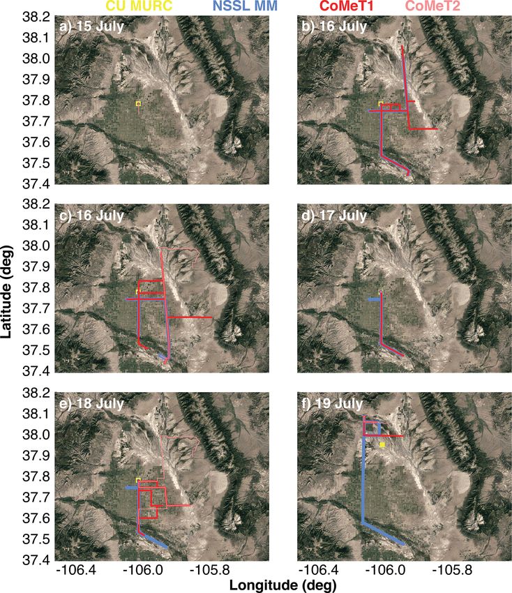
Finally, the UNL deployed two CoMeTs for LAPSE-RATE. Houston et al., 2016). Manufacturer specifications for these
These systems are built around Ford Explorers and feature a instruments are provided in Hanft and Houston (2018) and
forward-mounted suite of meteorological sensors and a dual are again listed in Table 2 of this paper. In addition to the
moonroof (see Fig. 3). The CoMeTs measure air temperature measured variables, the CoMeT data loggers (Campbell Sci-
and relative humidity at ∼ 2 m a.g.l. (above ground level) us-
https://doi.org/10.5194/essd-13-155-2021 Earth Syst. Sci. Data, 13, 155–169, 2021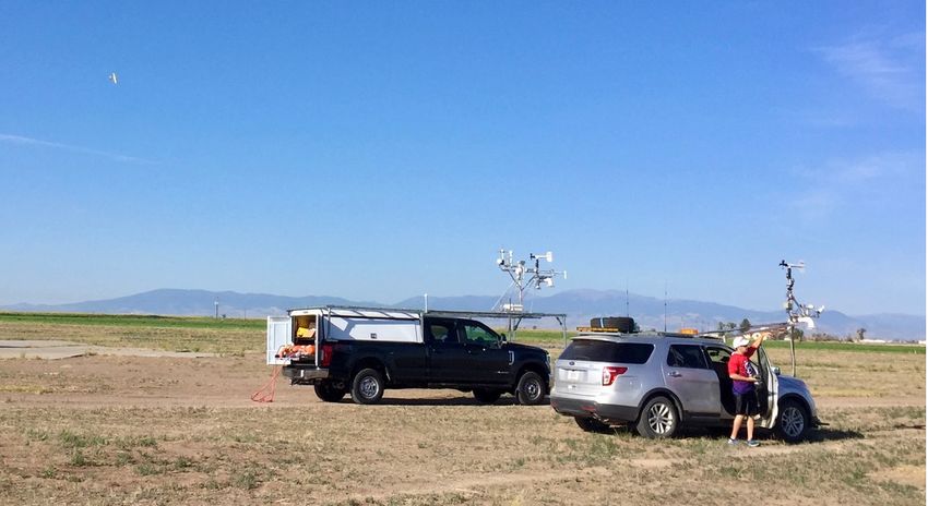
160                                      G. de Boer et al.: Measurements from mobile surface vehicles during LAPSE-RATE

entific CR6) along with a custom Python script use observed         at Leach Airport, and the transect between Leach Airport
quantities to calculate dewpoint temperature (Td ), mixing ra-      and the city of Alamosa. Finally, on 19 July, the NSSL MM
tio (qv ), potential temperature (θ ), equivalent potential tem-    covered an area from Alamosa to Saguache in the northwest
perature (θe ), virtual potential temperature (θv ), and wind       corner of the SLV. Most of the time on that date was spent
speed and direction. The equations used to compute these            sampling the square shown in the northwest part of the SLV
quantities are provided in Sect. 4.                                 in Fig. 6f to help understand the spatial variability of the
                                                                    drainage flow exiting the Saguache Valley. In total, the NSSL
                                                                    MM collected a total of 55.4 h of data, in addition to the mea-
3   Description of measurement locations,                           surements from the radiosondes launched.
    deployment strategies, and sampling                                The two UNL CoMeT vehicles were deployed separately
                                                                    throughout the San Luis Valley during the majority of the
The vehicles described above covered a significant amount of        LAPSE-RATE campaign. CoMeT-1 was principally focused
ground over the course of the campaign. Each played a differ-       on coordinated observations with the CU UAS team and in-
ent role in addressing the primary objectives of the LAPSE-         volved both stationary data collection based at Leach Airport
RATE campaign (see de Boer et al., 2020a, b). These ve-             and transect data collection across the SLV. CoMeT-2 was
hicles were used to evaluate the performance of UAS sen-            principally focused on stationary data collection in coordi-
sors, in addition to intercomparison between different sur-         nation with the UNL UAS team based at a site on the east-
face vehicles (see Fig. 4). Figure 5 provides an overview of        ern margins of the SLV in the northwest corner of the Great
the amount of time each vehicle spent making atmospheric            Sand Dunes National Park (henceforth referred to as obser-
measurements during the campaign. As shown, sampling pri-           vation site “Gamma”; Islam et al., 2019, 2020). As with the
marily occurred in the morning and early afternoon (local           NSSL MM, the CoMeT data collection began on 15 July with
time), with the NSSL MM generally starting the earliest in          CoMeT-1 operating transects based out of Leach Airport and
order to launch an early-morning radiosonde (see Bell et al.,       CoMeT-2 collecting stationary observations at Gamma. Sim-
2020). Sampling conducted on the afternoon of 14 July and           ilar operations were executed on 16 and 18 July during which
the morning of 20 July by the CU MURC was in support of             time CoMeT-1 performed extended east–west transects to the
platform intercomparison efforts (Barbieri et al., 2019).           far eastern portion of the SLV to help understand the role of
   The primary role of the CU MURC was to provide daily             surface type gradients and sloping terrain on that side of the
measurements at a consistent location (Leach Airport) in the        valley on convection initiation. On 18 July, following oper-
center of the sampling domain. In this role, the MURC acted         ations at Gamma, CoMeT-2 also executed a set of transects
as a meteorological tower that collected measurements in a          along the eastern margins of the irrigated region of the val-
similar manner from day to day, providing a baseline for            ley in an effort to explore whether surface flow parallel to
putting other observations collected during the campaign into       this margin resulted in a coherent convergence boundary. On
context. The only exception to this routine sampling took           17 July, both CoMeTs operated at Leach Airport. Finally,
place on 19 July, when all platforms were focused on cold           on 19 July, both CoMeTs joined the effort to capture the
air drainage out of the smaller valleys on the northern end of      early-morning Saguache Valley cold-air drainage, with fre-
the SLV. On 19 July, the MURC was positioned a bit farther          quent transects along County Road X between Saguache and
to the north, as can be seen in Fig. 6f to help evaluate the tim-   County Road 55. Over the course of the campaign, CoMeT-
ing and intensity of density currents flowing from Saguache         1 collected 50.4 h of data and CoMeT-2 collected 50.3 h of
(northwest corner of the SLV) and Villa Grove (northeast cor-       data.
ner of the SLV). In total, the MURC operated for seven days,           Figure 7 provides a statistical overview of data collected
capturing a total of 45.5 h of data.                                by these three platforms over the duration of the LAPSE-
   The NSSL MM filled multiple roles throughout the cam-            RATE campaign. Included are normalized probability distri-
paign. One important role included the launching of ra-             butions of measured quantities, including temperature, rela-
diosondes from various locations around the SLV (Bell et al.,       tive humidity, air pressure, wind speed, wind direction, and
2020). This often included early-morning radiosondes from           (for the NSSL MM and UNL CoMeT datasets) the differ-
Leach Airport. In addition, the NSSL MM was leveraged as            ence between the fast and slow temperature sensors. For all
a mobile measurement platform to capture information on             of these distributions, data were averaged to a moving 1 min
spatial variability throughout the broader valley. The first of     equally weighted window. The distributions illustrate differ-
these mobile measurement sorties took place on 15 July and          ences that are likely largely the result of instrument and plat-
included transects spanning the area between Alamosa, Col-          form location. For example, it is important to remember that
orado, and Moffatt, Colorado. These transects covered a vari-       while the NSSL MM and UNL CoMeT instruments were lo-
ety of different surface types, ranging from irrigated cropland     cated close to (< 3 m) the ground, the CU MURC data were
to dry desert-like areas on the eastern side of the SLV. On         collected atop a 15.2 m mast. Therefore, it is not surprising
16–18 July, the NSSL MM focused on the south-central por-           that the CU MURC pressure measurements are found to be
tion of the SLV, with much of the measurement time spent            slightly lower than those measured by the other two plat-

Earth Syst. Sci. Data, 13, 155–169, 2021                                             https://doi.org/10.5194/essd-13-155-2021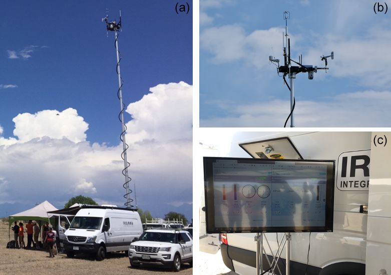
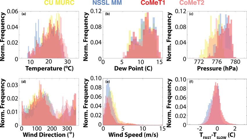
G. de Boer et al.: Measurements from mobile surface vehicles during LAPSE-RATE                                                 161

Figure 4. The NSSL MM and UNL CoMeT deployed side-by-side for an on-site intercomparison. The CU MURC was also located on site,
but out of the photograph, and a CU TTwistor UAS (see de Boer et al., 2020c, in this special issue) flies in the background.

Figure 5. Illustration of the uptime for the mobile surface vehicles deployed during LAPSE-RATE. Shown is the update for the CU MURC
(yellow), the NSSL MM (blue), and the UNL CoMeTs (red and pink). The thin dashed black lines indicate 06:00 LT (Mountain Daylight
Time), while the bold dashed black lines represent 12:00 LT for each day.

forms. Similarly, the CU MURC temperature and RH distri-            est in the early morning, with a gradual but notable warm-
butions lack the extremes, with measurements from the top           ing over the course of the day. Along with this, relative hu-
of the mast likely missing the coldest temperatures in the          midity levels were generally highest in the morning and de-
early morning, and the warmest temperatures in the after-           creased significantly over the course of the day. Interestingly,
noon. Also attributable to this altitude difference is the slight   the middle of the week did feature one day (17 July) where
but noticeable increase in wind speeds and counterclockwise         the MURC was sampling later into the afternoon, and tem-
shift in wind direction from the near-surface environment to        peratures were recorded dropping during that time period,
the height of the mast. Finally, for both the NSSL MM and           decreasing from around 26 ◦ C in the mid-afternoon to below
the UNL CoMeT data, the slow temperature sensor inside of           20 ◦ C by the end of sampling around 17:00 MDT. Figure 8b
the membrane (HMP155) was shown to have a warm bias                 provides insight into the variability occurring over the course
relative to the fast sensor (T109 SS), and the UNL CoMeT            of the field campaign. The earliest days (14–16 July) were
difference distribution is shown to have an extended tail to-       consistently warm and relatively humid. The atmosphere be-
wards positive values. The mean difference (fast minus slow)        came drier later in the campaign, with relative humidity val-
of the NSSL MM temperature sensors was −0.328 ◦ C, while            ues peaking at around 70 % on 19 July, despite tempera-
the mean difference of the UNL CoMeT temperature sensors            tures that were slightly cooler than those recorded on 17 and
was −0.398 ◦ C.                                                     18 July, when relative humidity levels climbed above 90 %
   Figure 8 provides additional insight into the temporal vari-     in the early-morning hours. In general, afternoons were il-
ability of the recorded variables, both in terms of diurnal cy-     lustrated to fall between 25–27 ◦ C, and mornings between
cle and over the extent of the LAPSE-RATE campaign, based           10–15 ◦ C (largely depending on the start time of sampling
on measurements obtained by the CU MURC. Figure 8a                  for a given date). Wind speed and direction measurements
shows that, as expected, temperatures were generally cold-          are shown in Fig. 8c and demonstrate that winds were gen-

https://doi.org/10.5194/essd-13-155-2021                                              Earth Syst. Sci. Data, 13, 155–169, 2021
162                                     G. de Boer et al.: Measurements from mobile surface vehicles during LAPSE-RATE

Figure 6. Position data for the different platforms over the length of the campaign, broken down on a day-by-day basis. The CU MURC
positions are indicated by the yellow square, while the NSSL mobile mesonet (blue) and UNL CoMeTs (red and pink) mobile datasets are
shown by the lines. Background maps are from © Google through their API.

erally quite light throughout the week, with values between         platform pitch and roll. All data were averaged across a mov-
0–6 m s−1 . An intensification of winds in the afternoon was        ing 1 s window. Any data points falling inside of the 1 s win-
seen on 14, 15, and 17 July, generally associated with con-         dow were included in averaging, though no filter was imple-
vective systems developing over the valley and surrounding          mented to ensure any particular number of samples within
mountain peaks. Wind directions were generally from the             a given 1 s averaging window. Time periods where no data
south and east. With the stronger winds resulting in a more         were collected are included as “NaN”. Screening for out-
northerly and westerly component. The only sampling period          liers was completed using the MATLAB “filloutliers” func-
with solidly westerly winds was the morning of 20 July.             tion, which detects and replaces outliers using a linear in-
                                                                    terpolation between points not deemed to be outliers. In the
                                                                    current application, outliers were defined as points falling
4     Data processing and quality control                           more than three local standard deviations outside of a mov-
                                                                    ing mean window encompassing 10 s worth of data. Note that
4.1    CU MURC                                                      this technique was applied to the measured zonal and merid-
Data available from the CU MURC have been processed in              ional wind components only, and not to the wind speed and
various ways to average the data, remove outliers, and cor-         direction included in the dataset that are calculated using the
rect the wind measurements from the sonic anemometer for

Earth Syst. Sci. Data, 13, 155–169, 2021                                              https://doi.org/10.5194/essd-13-155-2021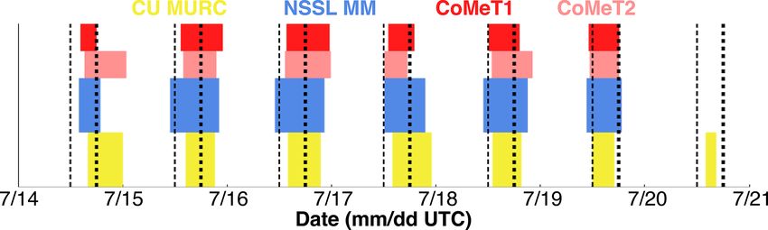
G. de Boer et al.: Measurements from mobile surface vehicles during LAPSE-RATE 163 Figure 7. Distributions of 1 min averages of data collected by the three platforms. Included are (a–f) distributions of air temperature, dew point temperature, pressure, wind direction, wind speed, and the difference between the fast and slow temperature sensors (where applicable). For all figures, CU MURC data are represented in yellow, NSSL MM data are represented in blue, and UNL CoMeT data are represented in red and pink. Figure 8. Panels illustrating the temporal variability of the temperature (a, b), dew point temperature (a, b), and wind data (c) collected by the CU MURC. Panel (a) shows diurnal variability, while (b) shows the variability by date. components, given that such averages are not possible on the Here, um , vm , and wm are the measured instantaneous veloc- vector values. ity components as measured by the sonic anemometer; A is Rotation of the CU MURC sonic anemometer data was the rotation matrix; and uf , vf , and wf are the final velocity completed using a standard three-axis rotation (Tropea et al., components. A can be approximated by combining multiple 2007), where the updated wind coordinates are calculated as rotations to align the coordinate system using measured Eu- follows: ler angles. In this case, we assume the following: uf um A = T · S · R, vf = A vm . wf wm https://doi.org/10.5194/essd-13-155-2021 Earth Syst. Sci. Data, 13, 155–169, 2021
164 G. de Boer et al.: Measurements from mobile surface vehicles during LAPSE-RATE
where computing power is enough to handle the calculations in real
time, making data display and recording easier.
1 0 0 For the derived winds, the measured wind speed and di-
T = 0 cos ψ sin ψ , rection directly off the anemometer is a combination of the
0 − sin ψ cos ψ vehicle motion vector and the ambient wind vector (this com-
bined vector is the vehicle relative vector), which need to
cos ϕ 0 sin ϕ
be separated. To obtain the ambient wind vector, the vehicle
S= 0 1 0 ,
motion must be subtracted from the vehicle relative vector
− sin ϕ 0 cos ϕ
in a process similar to that outlined in Sect. 4.1 for the CU
cos θ sin θ 0
MURC, though not as complex, as the wind monitor on the
R = − sin θ cos θ 0 , NSSL MM is only two-dimensional. The vehicle motion is
0 0 1 obtained from the onboard GPS and broken into N–S and
E–W components. The apparent wind vectors as measured
and ψ, ϕ, and θ are the roll, pitch, and yaw rotation angles, by the anemometer directly are also broken into components
respectively, as measured by the CU MURC operators. Note but are first added to the vehicle heading to obtain a true di-
that these angles were only measured once after parking the rectional vector rather than a vehicle relative vector. The ap-
vehicle and do not vary in time in between vehicle move- parent wind components are then subtracted from the vehicle
ments. Therefore, any swaying of the vehicle as a result of motion components to obtain the ambient wind components.
people getting in and out, wind, or for other reasons may im- The final step of the process involves converting the ambient
pact the wind measurements from the sonic anemometer and components back into vector form, which requires a tedious
may not be accounted for. Note that the rotations are applied series of manual computations to determine the quadrant rel-
in yaw, pitch, roll order, meaning that we step through the ative angle and its true meteorological heading. The vector
rotation as follows: wind speed is found simply with
p
u1 = um cos θ + vm sin θ, wind_speed = X 2 + Y 2 ,
v1 = −um sin θ + vm cos θ,
where X and Y are the ambient wind components for the U
w1 = wm , and V directions, respectively. For the vector wind direction,
the components must be examined to determine where on the
u2 = u1 cos ϕ + w1 sin ϕ,
meteorological coordinate system they lie and manually as-
v2 = v1 , sembled in the correct direction. This is due to the fact that
w2 = −u1 sin ϕ + w1 cos ϕ, traditional use of sin, cos, and tangent (and their inverse func-
tions) are referenced to a mathematical coordinate system
uf = u2 , which is reversed and offset by 90◦ from the meteorological
vf = v2 cos ψ + w2 sin ψ, coordinate system. To determine the wind direction, an offset
wf = −v2 sin ψ + w2 cos ψ. to either 90 or 270◦ is found by taking ATAN(ABS(Y /X)).
This value is then added or subtracted from the appropriate
Note that these corrections are only applied to the wind reference angle depending on the quadrant. For example, if Y
measurements from the sonic anemometer. The influence of and X were both +15 m s−1 , then ATAN(ABS(Y /X)) = 45◦ .
slight offsets in pitch and roll are negligible for the R.M. Since both Y and X are positive values, the resulting angle
Young propeller-based wind instrument as the propeller fol- should be in the first quadrant, or between 0 and 90◦ ; thus
lows a cosine response. For LAPSE-RATE, the sensor pitch the ATAN value is subtracted from the 90◦ reference angle,
and roll angles varied between −1.7 and 2.35◦ and −2.21 and obtaining an environmental wind direction of 45◦ . A more
3.48◦ , respectively. These angles correspond to a maximum detailed description of this process is forthcoming in a future
error of 0.2 %, well below the uncertainty of the instrument. paper. Note that if the vehicle is not moving, this component-
The sensor was aligned with magnetic north on a daily basis. based approach is not needed and the wind direction can be
found by simply rotating the observed winds by the vehicle
4.2 NSSL MM
heading while stationary.
The vehicle heading is also corrected in real time for cases
For the NSSL MMs, a majority of the data processing and where the vehicle is not moving. In these situations, the head-
variable calculation is done in real time on the CR6 data log- ing of the vehicle is obtained via a magnetic compass which
ger. Most of the observations do not require much in the way provides the magnetic bearing. This is used in cases where
of modification; the exceptions to that are derived ambient the vehicle motion is less than 1 m s−1 . The magnetic head-
winds, vehicle heading, and the environmental RH. This is ing differs from true north by an offset which is dependent on
an advantage of the CR6 data logging system, as the onboard the coordinates of the observation location, called the mag-
Earth Syst. Sci. Data, 13, 155–169, 2021 https://doi.org/10.5194/essd-13-155-2021G. de Boer et al.: Measurements from mobile surface vehicles during LAPSE-RATE 165
netic declination angle. This angle is provided along with the For both CoMeT-1 and CoMeT-2, relative humidity is ad-
GPS coordinates in real time and is used to correct the mag- justed to the fast temperature following Richardson et al.
netic heading. (1998) and Houston et al. (2016): vapor pressure is calcu-
While the NSSL MM measures temperature and humidity, lated using slow temperature and relative humidity, satura-
it does so with a set of sensors behind a protective membrane tion vapor pressure is calculated using fast temperature, and
that significantly delays the response time as described in the ratio of the two is used to calculate the corrected (fast)
Sect. 2.2. With this filter in place, the measured RH is lagged relative humidity. In CoMeT-1, the calculations are done in
behind the true environmental RH and must be re-derived. the Python script using the following:
This process follows that of Richardson et al. (1998) where
17.67 · T∗
e e∗ = 6.112 exp ,
DerivedRH = · 100, 243.5 + T∗
es
from Wexler (1976) and Bolton (1980), where e∗ is either va-
17.502 · TdC
e = 6.1365 · EXP , por pressure or saturation vapor pressure and T∗ is dew point
240.97 + TdC temperature (for vapor pressure) or fast temperature (for sat-
17.502 · Tfast uration vapor pressure). Dew point temperature is calculated
es = 6.1365 · EXP ,
240.97 + Tfast using
where Tfast and TdC (the calculated dewpoint from the 257.14γ
HMP155) are in degrees Celsius. The calculation for dew- Td = ,
18.678 − γ
point is done with a built-in CR6 function for dewpoint, 18.678 − Tslow /234.5
which uses the Tetens equation and the vapor pressure γ = ln (0.01 · RH∗ ) + Tslow ,
257.14 + Tslow
(Campbell Scientific, 2020).
As a final step to the process, after the data are collected where RH∗ is the uncorrected (slow) relative humidity and
and archived, each dataset is run through a QC procedure Tslow is the slow temperature. In contrast to CoMeT-1, the
where the individual data files from a single operations pe- calculation of dew point temperature, vapor pressure, and
riod are combined, and a set of QC flags applied. The intent saturation vapor pressure is done within the logger, and
of these flags are not to remove data, but rather flag data that slightly different expressions are used. For dew point tem-
are potentially suspicious and should be examined manually. perature
There are four QC flags, representing panel temperature ex- −5420
cess, vehicle stationary periods, excessive changes to vehicle Td = ,
p · qv
motion, and a general sanity check. More specific details of ln
the QC flags are contained in the readme files that accom- 62.2 · 2.53 × 109
pany the data; however, a brief description is presented here. e
A3 ln
The panel temperature flag identifies areas where the inter- A2
Td =
nal temperature of the CR6 data logger changes by a signif- e
icant amount. This identifies periods where the logger may A2 − ln
A1
be having inconsistency issues or power supply problems,
is used, where A1 = 0.61078, A2 = 17.558, and A3 =
which manifest themselves in the internal temperature mon-
241.88. The expression used in the logger for (saturation)
itoring first. The second QC flag is meant to identify periods
vapor pressure is from Lowe (1977):
where the vehicle is stationary, which could increase the po-
tential for bias in the observations, while the third flag looks e∗ = B0 + B1 T + B2 T 2 + B3 T 3 + B4 T 4 + B5 T 5 + B6 T 6 ,
for sharp changes to the speed or direction. The latter flag is
meant to identify areas where there could be a discrepancy where B0 = 6.107799961, B1 = 4.436518521 × 10⁻¹ ,
between the vehicle heading and the observed winds, such B2 = 1.428945805 × 10⁻² , B3 = 2.650648471 × 10⁻⁴ ,
as in a sharp turn. The final QC flag simply examines all the B4 = 3.031240396 × 10 , B5 = 2.034080948 × 10⁻⁸ , and
−6
observations for values that are well outside the normal op- B6 = 6.136820929 × 10⁻¹¹ .
erating range. The water vapor mixing ratio is calculated using
e
qv = 62.2
4.3 UNL CoMeTs p
As mentioned in Sect. 2, the CoMeT data loggers and Python and dew point temperature and vapor pressure as described
scripts are used to calculate key quantities of interest in real above. Potential temperature for both CoMeTs is calculated
time. These quantities include corrected relative humidity, using
water vapor mixing ratio, dew point temperature, the poten- ! Rd
tial temperature (θ ), virtual potential temperature (θv ), and 105 Cpd
θ = Tfast .
equivalent potential temperature (θe ). p
https://doi.org/10.5194/essd-13-155-2021 Earth Syst. Sci. Data, 13, 155–169, 2021166 G. de Boer et al.: Measurements from mobile surface vehicles during LAPSE-RATE
Virtual potential temperature is calculated using error across the intercomparison datasets and analysis of the
adjusted time series. The result was a −0.6 K correction ap-
θv = θ (1 + 0.61qv ). plied to all CoMeT-1 slow temperature data.
Figure 9 illustrates comparisons between measurements
from all of the mobile systems leveraged to produce this
Equivalent potential temperature is calculated in both dataset. Using the GPS position, time periods where indi-
CoMeTs following Bolton (1980): vidual vehicles were within 300 m of one another were se-
3376
lected for this comparison. Each panel represents a compar-
θe = Tm exp − 2.54 qv (1 + 0.81qv ) , ison of the data points, interpolated to a common 1 s time
TLCL
grid, during these close encounters. Note that the times do
Tfast + 273.15 0.286qv
not necessarily match from one inter-platform comparison to
Tm = θ ,
θ the next (i.e., the times change from column to column but
2840 are the same from one row to the next within a given column).
TLCL = 55 + , General agreement is shown between the different platforms,
3.5 ln(Tfast + 273.15) − ln(e) − 4.805
with some notable (but predictable) differences. First, the CU
MURC pressure is shown to be systematically lower than the
e = 0.01 · RH · es pressure measured by the other vehicles, which as discussed
e above is consistent with the fact that the CU MURC pressure
qv = 62.2
p measurements were collected on from the top of the 15.2 m
h
17.67(T −273.15)
i
mast. As also discussed previously in relation to Fig. 7, this
243.5+(T −273.15)
es = 6.112 , elevation difference additionally results in the MURC tem-
2840 peratures being slightly cooler than those observed at the sur-
TLCL = 55 + face, and the relative humidities being slightly higher. Again,
3.5 ln(T ) − ln(e) − 4.805
257.14γ wind speeds are also shown to be ever-so-slightly higher at
Td = , the CU MURC mast height than at the surface. There is quite
18.678 − γ
a bit of scatter in the wind direction comparison, particularly
18.678−T T
234.5 + 257.14+T for those time periods with very light winds, though the ma-
γ = ln(0.01 · RH) .
jority of the points still fall close to the one-to-one line. A
Due to a hole in the pressure tube underneath the CoMeT- primary exception to this is for time periods when the wind
2 vehicle, it was found to have erroneously low air pres- was northerly, resulting in clusters of points in the upper-
sure measurements when the vehicle was in motion during left- and lower-right-hand quadrants of the figures. For days
LAPSE-RATE. To correct this error, observations from times with higher wind speeds, a tighter clustering around the one-
when CoMeT-1 and CoMeT-2 were in motion and in close to-one line is noticeable. Ultimately, this figure illustrates
proximity were used to evaluate the level of inaccuracy of the good consistency between the platforms, offering confidence
CoMeT-2 measurement. Here “close proximity” was defined to data users who plan to leverage a combination of these
as any observations within 25 m of the same point, measured datasets.
within 90 s of one another. The observations with the small-
est distance between them were used, and duplicates were re-
moved such that an observation from either vehicle was not 5 Data availability and file structure
used twice. The pressure difference and CoMeT-2 anemome-
ter speed were then aligned with those from CoMeT-1 us- The data files from the LAPSE-RATE project are gener-
ing a second-order polynomial. Anemometer speed was used ally being archived under a LAPSE-RATE community es-
instead of vehicle speed because vehicle speed was often a tablished at the Zenodo data archive (https://zenodo.org/
multiple of 5, which made it difficult to compute an accu- communities/lapse-rate/, last access: 21 January 2021). From
rate fit. The polynomial fit was used to calculate a pressure here, LAPSE-RATE observations are available for public
correction for all CoMeT-2 data obtained when the vehicle download and use. Contributors were encouraged to provide
was in motion and the anemometer speed was greater than files in NetCDF format, with self-describing metadata pro-
10 m s−1 . Other variables calculated using pressure (e.g., Td , vided to the user inside the NetCDF file. To make it possible
qv , θ , θe , and θv ) were recalculated using the corrected pres- for scientists to cite LAPSE-RATE data in their publications,
sure. the organizers of the campaign recognized the value of digital
Evaluation of data collected during the 14 July intercom- object identifiers (DOIs). DOIs were automatically generated
parison along with an intercomparison conducted on 19 July by the Zenodo archive at the data version and product level.
revealed an approximately constant bias in slow temperature Data from the different sources described above are posted
in the CoMeT-1 data. The magnitude of this bias was ap- as individual data streams on the archive, with each of the
proximated through minimization of the root mean square platforms described in the previous section having their own
Earth Syst. Sci. Data, 13, 155–169, 2021 https://doi.org/10.5194/essd-13-155-2021G. de Boer et al.: Measurements from mobile surface vehicles during LAPSE-RATE 167
Figure 9. Vehicle-to-vehicle comparisons for time periods when vehicles were within 300 m of one another. Variables evaluated include (top
to bottom) temperature (◦ C), relative humidity (%), pressure (hPa), wind speed (m s−1 ), and wind direction (◦ ). The top row includes labels
to indicate which platform is on which axis, and these orientations are maintained through each column. For the temperature comparisons
(top row), both the slow (dark dots) and fast (lighter dots) temperature sensors are evaluated.
DOI. It is important to note that each platform may have sev- two versions, and users are encouraged to use version 2,
eral different levels of data available. Therefore, data prod- which includes corrected GPS data for the vehicle loca-
ucts with different levels of processing and quality control tions. These data are also available at the Zenodo website
may be provided with separate DOIs. This means the files (https://zenodo.org/record/3838724#.XvOMGi2z1TZ,
and data described in this publication are spread across a va- last access: 21 January 2021) under the DOI
riety of DOIs, and that additional DOIs could be created in https://doi.org/10.5281/zenodo.3838724.
the future that include LAPSE-RATE data, as additional data
products are developed.
As of the writing of this paper, the CU MURC dataset 6 Summary
(de Boer et al., 2020d) is available at the Zenodo web-
site (https://zenodo.org/record/3814765#.XrSRdS-z1TY, This paper provides an overview of data collected by three
last access: 21 January 2021) under the DOI types of mobile surface systems during the 2018 LAPSE-
https://doi.org/10.5281/zenodo.3814765. Data from the RATE campaign. These included the University of Colorado
NSSL MM include two versions (Waugh, 2020). The MURC, the NOAA National Severe Storms Laboratory Mo-
original version contained files with incorrect QC flags. bile Mesonet, and two University of Nebraska CoMeT vehi-
While the core data are correct, the QC flags can be useful cles. In combination, these vehicles collected over 140 h of
for determining specific areas of interest or problems. After meteorological data in the San Luis Valley of Colorado be-
identifying this issue, the files were reprocessed to include tween 14–20 July 2018. Data from these vehicles are avail-
the correct QC flags and were uploaded to the archive able for public download from the Zenodo website, and
as version 2. Users should use version 2, which is avail- the previous sections describe processing conducted on this
able at Zenodo.org (https://zenodo.org/record/3738175# dataset before publication and provide information on the ex-
.XrNLkC-z1TY, last access: 21 January 2021) under DOI pected accuracy of the sensors deployed on these systems.
https://doi.org/10.5281/zenodo.37175. Finally, the UNL The primary focus of the LAPSE-RATE campaign was to
CoMeT datasets (Houston and Erwin, 2020) also include collect data from a fleet of unmanned aerial vehicles and
surface in situ and remote-sensing systems, and to combine
https://doi.org/10.5194/essd-13-155-2021 Earth Syst. Sci. Data, 13, 155–169, 2021168 G. de Boer et al.: Measurements from mobile surface vehicles during LAPSE-RATE
those data with high-resolution numerical simulations to gain Sciences (grant no. AGS 1807199), and the US Department of En-
understanding on boundary layer processes and phenomena. ergy, Office of Science (grant no. DE-SC0018985).
The primary measurement objectives of the vehicles dis-
cussed in the current paper are shared above, along with the
locations of the operation of each throughout the campaign. Review statement. This paper was edited by David Carlson and
reviewed by Min Liu and one anonymous referee.
Author contributions. GB planned the LAPSE-RATE field cam-
paign, constructed this paper, and conducted data processing of the References
CU MURC data. SB, CD, and BA contributed to the collection of
the MURC data and were deployed to the field during LAPSE- Bailey, S. C. C., Sama, M. P., Canter, C. A., Pampolini, L. F., Lip-
RATE. AE, WS, and AH contributed to the collection of the UNL pay, Z. S., Schuyler, T. J., Hamilton, J. D., MacPhee, S. B.,
CoMeT data, processed and quality-controlled these data, and are Rowe, I. S., Sanders, C. D., Smith, V. G., Vezzi, C. N., Wight,
the primary points of contact for this dataset. They additionally H. M., Hoagg, J. B., Guzman, M. I., and Smith, S. W.: Uni-
helped with the writing of this paper. SW was solely responsible versity of Kentucky measurements of wind, temperature, pres-
for collection of the NSSL MM data and subsequent quality control sure and humidity in support of LAPSE-RATE using multisite
of the resulting dataset. Additionally, he contributed to the writing fixed-wing and rotorcraft unmanned aerial systems, Earth Syst.
of this paper. Sci. Data, 12, 1759–1773, https://doi.org/10.5194/essd-12-1759-
2020, 2020.
Barbieri, L., Kral, S. T., Bailey, S. C.C., Frazier, A. E., Jacob, J.
Competing interests. Gijs de Boer is the lead editor for the spe- D., Reuder, J., Brus, D., Chilson, P. B., Crick, C., Detweiler, C.,
cial issue in which this paper appears. Additionally, Gijs de Boer Doddi, A., Elston, J., Foroutan, H., González-Rocha, J., Greene,
works as a consultant for Black Swift Technologies, who partici- B. R., Guzman, M. I., Houston, A. L., Islam, A., Kemppinen,
pated in the LAPSE-RATE campaign. O., Lawrence, D., Pillar-Little, E. A., Ross, S. D., Sama, M.
P., Schmale, D. G., Schuyler, T. J., Shankar, A., Smith, S. W.,
Waugh, S., Dixon, C., Borenstein, S., and de Boer, G.: Intercom-
Special issue statement. This article is part of the special issue parison of Small Unmanned Aircraft System (sUAS) Measure-
“Observational and model data from the 2018 Lower Atmospheric ments for Atmospheric Science during the LAPSE-RATE Cam-
Process Studies at Elevation – a Remotely-piloted Aircraft Team paign, Sensors, 19, 2179, https://doi.org/10.3390/s19092179,
Experiment (LAPSE-RATE) campaign”. It is a result of the In- 2019.
ternational Society for Atmospheric Research using Remotely pi- Bell, T. M., Klein, P. M., Lundquist, J. K., and Waugh, S.: Remote
loted Aircraft (ISARRA 2018) conference, Boulder, USA, 9–12 sensing and radiosonde datasets collected in the San Luis Val-
July 2018. ley during the LAPSE-RATE campaign, Earth Syst. Sci. Data
Discuss. [preprint], https://doi.org/10.5194/essd-2020-314, in re-
view, 2020.
Acknowledgements. General support for salary and overhead as- Bolton, D.: The computation of equivalent potential temperature,
sociated with the collection of these datasets was provided by the Mon. Weather Rev., 108, 1046–1053, 1980.
NOAA Physical Sciences Division and the University of Colorado’s Brus, D., Gustafsson, J., Kempinen, O., de Boer, G., and Hirsikko,
Integrated Remote and In Situ Sensing (IRISS) grand challenge A.: Atmospheric aerosol, gases and meteorological parameters
project. We would additionally like to recognize financial support measured during the LAPSE-RATE campaign, Earth Syst. Sci.
for student participation and travel from the National Science Foun- Data Discuss. [preprint], https://doi.org/10.5194/essd-2020-251,
dation (NSF AGS 1807199) and the US Department of Energy (DE- in review, 2020.
SC0018985). General support for the LAPSE-RATE campaign was Campbell Scientific: CR Basic Help – CR Basic Editor, available
provided by the International Society for Atmospheric Research at: https://help.campbellsci.com/crbasic/cr6/, last access: 16 May
using Remotely-piloted Aircraft (ISARRA). CoMeT-1 was funded 2020.
through a grant from the Air Force Office of Scientific Research De- de Boer, G., Argrow, B., Cassano, J., Cione, J., Frew, E.,
fense University Research Instrumentation Program (FA2386-14-1- Lawrence, D., Wick, G., and Wolff, C.: Advancing unmanned
3010). CoMeT-2 was funded through an equipment allocation in- aerial capabilities for atmospheric research, B. Am. Meteorol.
cluded in the NSF Research Infrastructure Improvement Program: Soc., 100, ES105–ES108, https://doi.org/10.1175/BAMS-D-18-
Track-2 Focused EPSCoR Collaborations award (OIA-1539070). 0254.1, 2019.
Funding for the NSSL MM and travel was provided for through de Boer, G., Diehl, C., Jacob, J., Houston, A., Smith, S. W., Chil-
internal NSSL funds, with sounding expendables donated by Okla- son, P., Schmale III, D. G., Intrieri, J., Pinto, J., Elston, J., Brus,
homa State University. D., Kemppinen, O., Clark, A., Lawrence, D., Bailey, S. C.C.,
Sama, M. P., Frazier, A., Crick, C., Natalie, V., Pillar-Little, E.
A., Klein, P., Waugh, S., Lundquist, J. K., Barbieri, L., Kral, S. T.,
Financial support. This research has been supported by the Na- Jensen, A. A., Dixon, C., Borenstein, S., Hesselius, D., Human,
tional Science Foundation, Division of Atmospheric and Geospace K., Hall, P., Argrow, B., Thornberry, T., Wright, R., and Kelly,
J. T.: Development of community, capabilities and understand-
ing through unmanned aircraft-based atmospheric research: The
Earth Syst. Sci. Data, 13, 155–169, 2021 https://doi.org/10.5194/essd-13-155-2021G. de Boer et al.: Measurements from mobile surface vehicles during LAPSE-RATE 169 LAPSE-RATE campaign, B. Am. Meteorol. Soc., 101, E684– Natalie, V., Avery, A., Hemingway, B., Frazier, A., Crick, C., and E699, https://doi.org/10.1175/BAMS-D-19-0050.1, 2020a. Jacob, J.: Kinematic and thermodynamic atmospheric boundary de Boer, G., Houston, A., Jacob, J., Chilson, P. B., Smith, S. W., layer observations in the San Luis Valley, CO via unmanned air- Argrow, B., Lawrence, D., Elston, J., Brus, D., Kemppinen, O., craft systems during the LAPSE-RATE field campaign, Earth Klein, P., Lundquist, J. K., Waugh, S., Bailey, S. C. C., Frazier, Syst. Sci. Data Discuss., in preparation, 2021. A., Sama, M. P., Crick, C., Schmale III, D., Pinto, J., Pillar-Little, Pietrycha, A. E. and Rasmussen, E. N.: Finescale Surface Obser- E. A., Natalie, V., and Jensen, A.: Data generated during the 2018 vations of the Dryline: A Mobile Mesonet Perspective, Weather LAPSE-RATE campaign: an introduction and overview, Earth Forecast., 19, 1075–1088, https://doi.org/10.1175/819.1, 2004. Syst. Sci. Data, 12, 3357–3366, https://doi.org/10.5194/essd-12- Pillar-Little, E. A., Greene, B. R., Lappin, F. M., Bell, T. M., 3357-2020, 2020b. Segales, A. R., de Azevedo, G. B. H., Doyle, W., Kanneganti, S. de Boer, G., Dixon, C., Borenstein, S., Lawrence, D. A., Elston, T., Tripp, D. D., and Chilson, P. B.: Observations of the thermo- J., Hesselius, D., Stachura, M., Laurence III, R., Swenson, S., dynamic and kinematic state of the atmospheric boundary layer Choate, C. M., Doddi, A., Sesnic, A., Glasheen, K., Laouar, Z., over the San Luis Valley, CO using remotely piloted aircraft sys- Quinby, F., Frew, E., and Argrow, B. M.: University of Colorado tems during the LAPSE-RATE field campaign, Earth Syst. Sci. and Black Swift Technologies RPAS-based measurements of the Data Discuss. [preprint], https://doi.org/10.5194/essd-2020-194, lower atmosphere during LAPSE-RATE, Earth Syst. Sci. Data in review, 2020. Discuss. [preprint], https://doi.org/10.5194/essd-2020-333, in re- Pinto, J. O., Jensen, A. A., Jiménez, P. A., Hertneky, T., Muñoz- view, 2020c. Esparza, D., Dumont, A., and Steiner, M.: Realtime WRF de Boer, G., Borenstein, S., Dixon, C., and Argrow, B.: University of LES Simulations to Support UAS Flight Planning and Opera- Colorado MURC Observations from LAPSE-RATE [Data set], tions During 2018 LAPSE-RATE, Earth Syst. Sci. Data Dis- Zenodo, https://doi.org/10.5281/zenodo.3814765, 2020d. cuss. [preprint], https://doi.org/10.5194/essd-2020-242, in re- Fernández-Cabán, P. L., Alford, A. A., Bell, M. J., Biggerstaff, M. view, 2020. I., Carrie, G. D., Hirth, B., Kosiba, K., Phillips, B. M., Schroeder, Richardson, S. J., Frederickson, S. E., Brock, F. V., and Brotzge, J. L., Waugh, S. M., Williford, E., Wurman, J., and Masters, F. J. A.: Combination temperature and relative humidity probes: J.: Observing Hurricane Harvey’s Eyewall at Landfall, B. Am. Avoiding large air temperature errors and associated relative hu- Meteorol. Soc., 100, 759–775, https://doi.org/10.1175/BAMS- midity errors, Preprints, 10th Symp. On Meteorological Obser- D-17-0237.1, 2019. vations and Instrumentation, Phoenix, AZ, 11–16 January 1998, Hanft, W. and Houston, A. L.: An observational and model- Amer. Meteor. Soc., 278–283, 1998. ing study of mesoscale air masses with high theta-e, Mon. Riganti, C. J. and Houston, A. L.: Rear-Flank Outflow Dynam- Weather Rev., 146, 2503–2524, https://doi.org/10.1175/MWR- ics and Thermodynamics in the 10 June 2010 Last Chance, D-17-0389, 2018. Colorado, Supercell, Mon. Weather Rev., 145, 2487–2504, Houston, A. and Erwin, A.: University of Nebraska-Lincoln Mo- https://doi.org/10.1175/MWR-D-16-0128.1, 2017. bile Mesonet files from LAPSE-RATE [Data set], Zenodo, Straka, J. M., Rasmussen, E. N., and Fredrickson, S. E.: A mo- https://doi.org/10.5281/zenodo.3709611, 2020. bile mesonet for finescale meteorological observations, J. At- Houston, A. L., Laurence III, R. J., Nichols, T. W., Waugh, mos. Ocean. Tech., 13, 921–936, https://doi.org/10.1175/1520- S., Argrow, B., and Ziegler, C. L.: Intercomparison of 0426(1996)0132.0.CO;2, 1996. unmanned aircraft-borne and mobile mesonet atmo- Tropea, C., Yarin, A. L., and Foss, J. F. (Eds.): Springer spheric sensors, J. Atmos. Ocean. Tech., 33, 1569–1582, Handbook of Experimental Fluid Mechanics, Berlin, Springer, https://doi.org/10.1175/JTECH-D-15-0178.1, 2016. https://doi.org/10.1007/978-3-540-30299-5, 2007. Islam, A., Houston, A. L., Shankar, A., and Detweiler, C.: Waugh, S.: The “U-tube”: An improved aspirate temperature sys- Design and Evaluation of Sensor Housing for Bound- tem for mobile meteorological observations, especially in severe ary Layer Profiling Using Multirotors, Sensors, 19, 2481, weather, MS thesis, Univ. of Oklahoma, 87 pp., 2012. https://doi.org/10.3390/s19112481, 2019. Waugh, S.: National Severe Storms Laboratory Mobile Islam, A., Shankar, A., Houston, A., and Detweiler, C.: University Mesonet data files from Lapse-Rate [Data set], Zenodo, of Nebraska UAS profiling during LAPSE-RATE, Earth Syst. https://doi.org/10.5281/zenodo.3738175, 2020. Sci. Data Discuss. [preprint], https://doi.org/10.5194/essd-2020- Waugh, S. and Frederickson, S. E.: An improved aspirated tempera- 374, in review, 2020. ture system for mobile meteorological observations, especially in Lowe, P. R.: An Approximating Polynomial for the Com- severe weather, 25th Conf. on Severe Local Storms, Denver, CO, putation of Saturation Vapor Pressure, J. Appl. Mete- Amer. Meteor. Soc., P 5.2, available at: https://ams.confex.com/ orol. Clim., 16, 100–103, https://doi.org/10.1175/1520- ams/25SLS/techprogram/paper_176205.htm (last access: 21 Jan- 0450(1977)0162.0.CO;2, 1977. uary 2021), 2010. Markowski, P. M.: Mobile Mesonet Observations on 3 May 1999, Wexler, A.: Vapor Pressure Formulation for Water in Range 0 to Weather Forecast., 17, 430–444, https://doi.org/10.1175/1520- 100°C, A Revision, Journal of Research of the National Bureau 0434(2002)0172.0.CO;2, 2002. of Standards, 80A, 775–785, 1976. https://doi.org/10.5194/essd-13-155-2021 Earth Syst. Sci. Data, 13, 155–169, 2021
You can also read