The completed SDSS-IV extended Baryon Oscillation Spectroscopic Survey: 1000 multi-tracer mock catalogues with redshift evolution and systematics ...
←
→
Page content transcription
If your browser does not render page correctly, please read the page content below
MNRAS 503, 1149–1173 (2021)                                                                                                       doi:10.1093/mnras/stab510
Advance Access publication 2021 February 24

The completed SDSS-IV extended Baryon Oscillation Spectroscopic
Survey: 1000 multi-tracer mock catalogues with redshift evolution and
systematics for galaxies and quasars of the final data release
Cheng Zhao ,1‹ Chia-Hsun Chuang ,2 Julian Bautista ,3 Arnaud de Mattia,4 Anand Raichoor,1

                                                                                                                                                                 Downloaded from https://academic.oup.com/mnras/article/503/1/1149/6149160 by University of Portsmouth Library user on 18 May 2021
Ashley J. Ross ,5 Jiamin Hou,6 Richard Neveux,4 Charling Tao,7 Etienne Burtin,4 Kyle S. Dawson,8
Sylvain de la Torre,9 Héctor Gil-Marı́n ,10,11 Jean-Paul Kneib,1,9 Will J. Percival,12,13,14 Graziano Rossi,15
Amélie Tamone,1 Jeremy L. Tinker ,16 Gong-Bo Zhao,17,18 Shadab Alam19 and Eva-Maria Mueller20
1 Institute of Physics, Laboratory of Astrophysics, École Polytechnique Fédérale de Lausanne (EPFL), Observatoire de Sauverny, CH-1290 Versoix, Switzerland
2 Kavli  Institute for Particle Astrophysics and Cosmology, Stanford University, 452 Lomita Mall, Stanford, CA 94305, USA
3 Institute of Cosmology & Gravitation, Dennis Sciama Building, University of Portsmouth, Portsmouth PO1 3FX, UK
4 IRFU,CEA, Université Paris-Saclay, F-91191 Gif-sur-Yvette, France
5 Center for Cosmology and Astro-Particle Physics, Ohio State University, Columbus, OH 43210, USA
6 Max-Planck-Institut für Extraterrestrische Physik, Postfach 1312, Giessenbachstr., 85748 Garching bei München, Germany
7 CPPM, Aix-Marseille Université, CNRS/IN2P3, CPPM UMR 7346, F13288 Marseille, France
8 Department Physics and Astronomy, University of Utah, 115 S 1400 E, Salt Lake City, UT 84112, USA
9 Aix Marseille Univ, CNRS, CNES, LAM, F13388 Ma rseille, France
10 Institut de Ciències del Cosmos, Universitat de Barcelona, ICCUB, Martı́ i Franquès 1, E08028 Barcelona, Spain
11 Institut d’Estudis Espacials de Catalunya (IEEC), E08034 Barcelona, Spain
12 Waterloo Centre for Astrophysics, University of Waterloo, Waterloo, ON N2L 3G1, Canada
13 Department of Physics and Astronomy, University of Waterloo, Waterloo, ON N2L 3G1, Canada
14 Perimeter Institute for Theoretical Physics, 31 Caroline St. North, Waterloo, ON N2L 2Y5, Canada
15 Department of Physics and Astronomy, Sejong University, Seoul 143-747, Korea
16 Center for Cosmology and Particle Physics, Department of Physics, New York University, New York, NY 10003, USA
17 National Astronomy Observatories, Chinese Academy of Science, Beijing 100101, P.R. China
18 School of Astronomy and Space Science, University of Chinese Academy of Sciences, Beijing 100049, P.R.China
19 Institute for Astronomy, University of Edinburgh, Royal Observatory, Edinburgh EH9 3HJ, UK
20 Department of Astrophysics, Department of Physics, University of Oxford, Denys Wilkinson Building, Keble Road, Oxford OX1 3RH, UK

Accepted 2021 February 18. Received 2021 February 10; in original form 2020 July 21

ABSTRACT
We produce 1000 realizations of synthetic clustering catalogues for each type of the tracers used for the baryon acoustic oscillation
and redshift space distortion analysis of the Sloan Digital Sky Surveys-IV extended Baryon Oscillation Spectroscopic Survey final
data release (eBOSS DR16), covering the redshift range from 0.6 to 2.2, to provide reliable estimates of covariance matrices and
test the robustness of the analysis pipeline with respect to observational systematics. By extending the Zel’dovich approximation
density field with an effective tracer bias model calibrated with the clustering measurements from the observational data, we
accurately reproduce the two- and three-point clustering statistics of the eBOSS DR16 tracers, including their cross-correlations in
redshift space with very low computational costs. In addition, we include the gravitational evolution of structures and sample selec-
tion biases at different redshifts, as well as various photometric and spectroscopic systematic effects. The agreements on the auto-
clustering statistics between the data and mocks are generally within 1 σ variances inferred from the mocks, for scales down to a
few h−1 Mpc in configuration space, and up to 0.3 h Mpc−1 in Fourier space. For the cross correlations between different tracers,
the same level of consistency presents in configuration space, while there are only discrepancies in Fourier space for scales above
0.15 h Mpc−1 . The accurate reproduction of the data clustering statistics permits reliable covariances for multi-tracer analysis.
Key words: methods: numerical – catalogues – cosmology: large-scale structure of Universe.

                                                                                  of structures. In particular, the baryon acoustic oscillation (BAO;
1 I N T RO D U C T I O N
                                                                                  Eisenstein & Hu 1998) feature is known as a standard ruler for
The spatial clustering of large-scale structures (LSS) offers in-                 geometrical measurements and provides constraints on the nature
sights into the expansion history of the Universe and the growth                  of dark energy (Eisenstein 2005). Redshift-space distortions (RSD;
                                                                                  Kaiser 1987) of the clustering statistics can be used to estimate
                                                                                  the structure formation rate and test gravity theories (Percival &
   E-mail: cheng.zhao@epfl.ch                                                    White 2009; Raccanelli et al. 2013). Precise cosmological constraints


C 2021 The Author(s)

Published by Oxford University Press on behalf of Royal Astronomical Society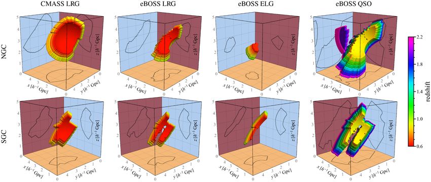
1150        C. Zhao et al.
with clustering measurements require the 3D positions – 2D angular          that methods with bias models, including EZmock and PATCHY, are
position and redshift – of tracers of the dark matter density field         not only among the most accurate ones, but also significantly faster
over a large volume, and possibly several different types of tracers        than methods with comparable precisions (Chuang et al. 2015b; Blot
to probe different cosmic epochs.                                           et al. 2019; Colavincenzo et al. 2019; Lippich et al. 2019). Actually,
   Recent large-scale galaxy spectroscopic surveys, such as the             PATCHY has been used for the BOSS DR12 analyses (e.g. Kitaura
Baryon Oscillation Spectroscopic Survey (BOSS; Dawson et al.                et al. 2016; Alam et al. 2017). We choose EZmock for this work, due
2013) – which belongs to the phase III of the Sloan Digital Sky             to its higher efficiency, and fewer free parameters of the bias model,
Surveys (SDSS) – have measured the redshifts of over one million            which makes it easier to be calibrated.
luminous red galaxies (LRG) with redshifts up to 0.75, covering                The EZmock algorithm uses Zel’dovich approximation

                                                                                                                                                         Downloaded from https://academic.oup.com/mnras/article/503/1/1149/6149160 by University of Portsmouth Library user on 18 May 2021
more than 9000 deg2 , and achieved per cent-level measurements of           (Zel’dovich 1970) to construct the density field at a given redshift, and
both distance scales and growth rate of structures (Alam et al. 2017).      populate matter tracers (haloes/galaxies/quasars) in the field with a
In addition, the extended BOSS (eBOSS; Dawson et al. 2016), as              parametrized modelling of tracer bias. This effective bias description
part of SDSS-IV (Blanton et al. 2017) and a complement to BOSS,             includes linear, nonlinear, deterministic and stochastic effects, which
has probed ∼0.8 million LRGs, star-forming emission line galaxies           have to be calibrated with clustering statistics from observations or
(ELG), and quasi stellar objects (QSO) in total, with the redshift range    N-body simulations, including typically the two-point correlation
0.6 < z < 2.2, for the LSS analysis of its final data release (DR16,        function (2PCF), power spectrum, and bispectrum. EZmock is able to
see Section 2.1; Ross et al. 2020; Raichoor et al. 2021). In addition,      reproduce both two- and three-point statistics of a reference N-body
∼0.2 million BOSS/eBOSS QSOs at z > 2.1 are used for Lyman-α                simulation precisely down to mildly nonlinear scales. For instance,
absorption measurements (du Mas des Bourboux et al. 2020; Lyke              the discrepancies of redshift space power spectrum produced by
et al. 2020), which extend the clustering analysis to higher redshift.      EZmock are less than 5 per cent for k  0.3 h Mpc−1 (Chuang et al.
   Apart from the sample size, accurate estimates of the uncertainties      2015b). Moreover, thanks to the incomparable efficiency of ZA,
in the clustering statistics are also essential for LSS analysis. One can   the remarkably low computational cost makes EZmock extremely
obtain the covariance matrices directly from the observational cata-        suitable for estimating covariances for large-scale analysis.
logues, by sampling the data in subvolumes with jackknife or boot-             In this work, we use the revised EZmock method to construct
strap estimations. However, variances on scales larger than the size of     mock catalogues for all eBOSS direct LSS tracers, including LRGs,
the subvolumes cannot be sampled, and systematic errors that apply          ELGs, and QSOs. For the estimates of the covariance matrices,
to all subsamples are not accounted for. An alternative way is to rely      we produce 1000 realizations of mock catalogues for each type
on the theoretical model for clustering statistics, and derive Gaussian     of the tracers. They are constructed from 46 000 simulation boxes
covariances (e.g. Grieb et al. 2016; Wadekar & Scoccimarro 2019).           with the side length of 5 h−1 Gpc, at several different redshifts, to
Further improvements can be achieved by rescaling the shot noise            account for the redshift evolution of structures. Furthermore, the
power to include non-Gaussianity (Philcox et al. 2020). Nevertheless,       mock tracers are populated from shared density fields, to ensure
the robustness of analytical approaches depend on the accuracies of         reliable estimates of the cross covariances. Besides, two sets of mocks
the models in nonlinear regimes of the cosmic evolution, and it is          are generated, complete and realistic, i.e. without and with applying
challenging for them to include observational systematic errors.            observational systematic effects. They are used for the analysis of
   In principle, these issues can be solved with catalogues generated       the eBOSS LRG samples (Gil-Marı́n et al. 2020; Bautista et al.
by N-body simulations: they encode the full nonlinear gravitational         2021), ELG samples (Tamone et al. 2020; de Mattia et al. 2021;
evolution, and can be applied known observational effects to sample         Raichoor et al. 2021), QSO samples (Neveux et al. 2020; Hou et al.
systematic errors. However, the estimate of covariance matrices             2021), and the final cosmological constraints (eBOSS Collaboration
requires a large number of realizations, and this is generally too          2020), with the systematic errors assessed using N-body simulations
computational expensive to be practical for N-body simulations with         (Alam et al. 2020a; Avila et al. 2020; Rossi et al. 2020; Smith
sufficient mass resolution and volume for current large-scale galaxy        et al. 2020). Moreover, Lin et al. (2020) use the GLAM method
surveys. To circumvent this problem, some more efficient but less           to construct the density field and adopt the bias model of the QPM
accurate methods for constructing mock catalogues are proposed,             method to generate mock catalogues for eBOSS ELGs. The eBOSS
such as the bias assignment method (BAM; Balaguera-Antolı́nez               DR16 EZmock catalogues presented in this work will be publicly
et al. 2019), COmoving Lagrangian Acceleration (COLA; Tassev,               available.1 In addition, all SDSS BAO and RSD measurements and
Zaldarriaga & Eisenstein 2013; Izard, Crocce & Fosalba 2016; Koda           the cosmological interpretations can be found on the SDSS website.2
et al. 2016), effective Zel’dovich approximation mock (EZmock;                 This paper is organized as follows. In Section 2, we describe the
Chuang et al. 2015a), FastPM (Feng et al. 2016), GaLAxy Mocks               methodology for constructing the mock catalogues. The clustering
(GLAM; Klypin & Prada 2018), lognormal (Coles & Jones 1991;                 statistics of the mock catalogues are shown in Section 3. We perform
Agrawal et al. 2017), peak patch (Bond & Myers 1996; Stein, Al-             the cross correlation analysis between different tracers in Section 4.
varez & Bond 2019), PerturbAtion Theory Catalog generator of Halo           Finally, in Section 5, we present the conclusions.
and galaxY distributions (PATCHY; Kitaura, Yepes & Prada 2014),
and quick particle mesh (QPM; White, Tinker & McBride 2014).
   These fast mock generation methods can be classified into three          2 METHODOLOGY
general categories. COLA, FastPM, GLAM, peak patch, and QPM                 We present in this section the improved version of the EZmock
are predictive algorithms that solve the dynamic evolution of               method, compared to the algorithm introduced in Chuang et al.
structures approximately. BAM, EZmock, and PATCHY generate
the dark matter density field using perturbation theories, and then
populate tracers with effective descriptions of their biases. While the     1 https://data.sdss.org/sas/dr16/eboss/lss/catalogs/EZmocks
lognormal method models halo distributions through modifications            2 The BAO and RSD measurements are available at https://sdss.org/science/f
of the matter density field. In particular, comparisons of some of the      inal-bao-and-rsd-measurements, and see https://sdss.org/science/cosmology
mock construction techniques with N-body simulations have shown             -results-from-eboss for the cosmological results.

MNRAS 503, 1149–1173 (2021)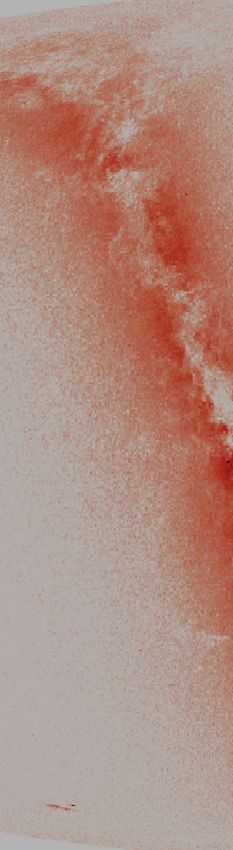
EZmock catalogues for eBOSS DR16                             1151

                                                                                                                                                              Downloaded from https://academic.oup.com/mnras/article/503/1/1149/6149160 by University of Portsmouth Library user on 18 May 2021
      Figure 1. The sky coverage of eBOSS DR16 tracers and BOSS DR12 LRGs, as well as the density map of Gaia DR2 sources with g < 15 mag.

(2015a). In particular, the method used for this work does not require         The sky coverage of the BOSS DR12 and eBOSS DR16 data,
the enhancement of the BAO signal for the initial conditions, and           with various masks applied, are illustrated in Fig. 1,4 where the
relies on less bias parameters to be calibrated. Moreover, the calibra-     background colour map indicates the angular source density of the
tion is done directly with the observed clustering measurements of          Gaia DR2 public data (Gaia Collaboration 2018), with a selection
the BOSS and eBOSS catalogues, without taking N-body simulations            of the g band magnitude (phot g mean mag < 15). In particular,
as references. This is because no reliable N-body simulation multi-         the left and right patches of the BOSS/eBOSS footprints are dubbed
tracer catalogue is available when the mocks are constructed, and           northern and southern Galactic caps (NGC and SGC) respectively.
the accuracy of the EZmock method has been validated using the              Since the two Galactic caps are spatially far away from each other, we
BigMultiDark simulation (Chuang et al. 2015b). As the result,               construct EZmock catalogues for NGC and SGC independently, but
the effective bias model of EZmock further accounts for the halo            with the same input parameters. Therefore, the expected clustering
occupation distributions (HOD; e.g. Berlind & Weinberg 2002) of             statistics of EZmock catalogues in both Galactic caps are identical,
different matter tracers. We have made the python interface for             if no radial selection (see Section 2.3.4) is applied.
constructing and calibrating EZmock catalogues publicly available.3            The total effective area of the CMASS LRG, eBOSS LRG, eBOSS
                                                                            ELG, and eBOSS QSO samples is 9376, 4103, 727, and 4702 deg2 ,
                                                                            respectively (Reid et al. 2016; Ross et al. 2020; Raichoor et al. 2021).
2.1 Reference data catalogues                                               The effective overlapped area between the eBOSS LRG and ELG
The catalogues for LSS analysis in eBOSS DR16 consist of ∼0.20              samples is 458 deg2 , and it is 509 deg2 for the overlapping region
million LRGs, ∼0.27 million ELGs, and ∼0.34 million QSOs, with              between eBOSS ELG and QSO samples.
the redshift ranges of                                                         Fig. 2 shows the effective radial comoving number densities of the
                                                                            tracers, evaluated in the framework of flat CDM cosmology, with
0.6 < z LRG < 1.0,                                                   (1)    m = 0.31. To estimate the statistical uncertainty of the observed
                                                                            data, the mock catalogues should be constructed with at least the peak
0.6 < z ELG < 1.1,                                                   (2)    number densities of different tracers. Meanwhile, we would like to
                                                                            avoid generating much more tracers than necessary to reduce the
0.8 < z QSO < 2.2.                                                   (3)    computational costs. Consequently, the number densities of LRGs,
                                                                            ELGs, and QSOs that we set for the generation of the mock catalogues
Moreover, a subsample of the BOSS DR12 complete-mass (CMASS)                are
LRGs with the same redshift range as equation (1) is also included for
                                                                                           −4 3
the cosmological analysis. As the result, the combined LRG sample            LRG = 3.2 × 10
                                                                            nbox             h Mpc−3 ,                                                  (4)
contains ∼0.38 million galaxies. For each of the sample, regions with
                                                                                           −4 3
low spectra completeness and qualities are masked to ensure reliable         ELG = 6.4 × 10
                                                                            nbox             h Mpc−3 ,                                                  (5)
clustering measurements. Besides, various weights are applied to
                                                                                           −5 3
correct for known observational systematics, and minimize the bias           QSO = 2.4 × 10
                                                                            nbox             h Mpc−3 ,                                                  (6)
of the clustering statistics (see Ross et al. 2020; Raichoor et al. 2021,
for details).                                                               respectively.

3 https://github.com/cheng-zhao/pyEZmock                                    4 See   https://skfb.ly/6TPBH and https://skfb.ly/6TPBI for 3D illustrations.

                                                                                                                     MNRAS 503, 1149–1173 (2021)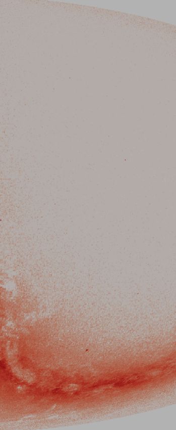
1152         C. Zhao et al.
                                                                              linear solution of the Lagrangian Perturbation Theory (LPT; see e.g.
                                                                              Bernardeau et al. 2002). In the Lagrangian description, the Eulerian
                                                                              position x of a particle at time t is expressed by its initial comoving
                                                                              position q (i.e. the position in the Gaussian random field) and a
                                                                              displacement :
                                                                              x(q, t) = q + (q, t).                                             (7)
                                                                              And the linear solution to the equation of motion yields

                                                                                                                                                        Downloaded from https://academic.oup.com/mnras/article/503/1/1149/6149160 by University of Portsmouth Library user on 18 May 2021
                                                                              ∇q ·  ZA (q, t) = −D1 (t)δ(q).                                    (8)
                                                                              Here  ZA stands for the displacement field in the Zel’dovich
                                                                              approximation, D1 (t) denotes the linear growth factor, and δ(q)
                                                                              indicates the initial density contrast in Lagrangian coordinates, which
                                                                              is sampled in Fourier space with random phases, with the amplitude
                                                                              being defined by the linear matter power spectrum Plin (k):
                                                                              Plin (k) = |δ(k)|2 .                                             (9)
Figure 2. The weighted comoving number densities of eBOSS DR16 tracers
and BOSS DR12 CMASS LRGs, with all the photometric and spectroscopic            In the framework of CDM, the linear growth factor can be
systematic weights included. The comoving distances and volumes are           evaluated numerically through the integral representation (Heath
evaluated in the flat CDM cosmology with m = 0.31. The three horizontal     1977; Carroll, Press & Turner 1992):
dashed lines show the number densities of the cubic LRG, ELG, and QSO
                                                                                                 5m a       dã
EZmock catalogues, i.e. 3.2 × 10⁻⁴ , 6.4 × 10⁻⁴ , and 2.4 × 10⁻⁵ h3 Mpc−3 ,   D1 (a) = a 3 H (a)           3 H 3 (ã)
                                                                                                                      ,                   (10)
respectively.
                                                                                                  2   0 ã
                                                                              where a indicates the scale factor, and H(a) is the Hubble function.
  Since all BOSS and eBOSS tracers share the sky area and redshift              The displacement field in the ZA can be obtained through the
range to some extent, in order to combine their results for final             Fourier transform of equation (8):
cosmological analysis, it is crucial to account for the cross covariance
between different tracers. To this end, we construct the mock                                         d3 k i k·q ik
                                                                               ZA (q, a) = D1 (a)          e       δ̂(k),                     (11)
catalogues for different tracers – including BOSS CMASS LRGs,                                        (2π )3      k2
and eBOSS LRGs/ELGs/QSOs – in the same comoving volume, and                   where δ̂(k) denotes the density contrast in Fourier space. Thus, the
with identical initial conditions, to ensure the same underlying dark         ZA density field ρ m can be efficiently computed with Fast Fourier
matter density field for all of them.                                         Transforms (FFT). In this work, FFTs are performed with the grid
                                                                              size of 10243 , in the 53 h−3 Gpc3 cubic volume.
2.2 Cubic mock catalogue generation                                              Once the displacement field is computed on the grid points, dark
                                                                              matter particles are moved from their initial Lagrangian positions
The starting point of our mock generation process is a Gaussian               – Cartesian grid points – to the final Eulerian positions following
random field in a periodic cubic volume, with a given initial power           equation (7). The dark matter density field is evaluated on the same
spectrum. The side length of the Gaussian random field in this work           grids, using the Cloud-in-Cell (CIC; Hockney & Eastwood 1981)
is 5 h−1 Gpc, which is large enough to cover the survey volume of             particle assignment scheme. Consequently, the number density fields
all tracers for clustering analysis. The same white noises are used for       of the observational tracers described hereafter, are all based on this
the construction of the Gaussian random field for different tracers.          grid size. In general, the EZmock parameters have to be re-calibrated,
   The fiducial cosmological model for constructing the mocks is              with a different number of grids in the same comoving volume.
flat CDM, with m = 0.307115, b = 0.048206, h = 0.6777,
σ 8 = 0.8225, and ns = 0.9611, which are the best-fitting values
from the Planck 2013 results (Planck Collaboration 2014). This is             2.2.2 Deterministic bias relations
the same cosmological model used by the PATCHY mock catalogues
for the final BOSS data release (Kitaura et al. 2016) which is                To populate tracers in the simulation box, we need to introduce a bias
calibrated based on the MultiDark simulations (Klypin et al. 2016).           model describing the relationship between tracers and dark matter, or
The linear matter power spectrum we use is generated by the CAMB5             in other words, to construct the tracer number density field ρ t based
software (Lewis, Challinor & Lasenby 2000). It has been shown                 on the dark matter density field ρ m . This process can be expressed
that the covariance matrix of two-point clustering measurements are           by a general bias function B:
insensitive to the input power spectrum, if the two- and three-point          ρt = B(ρm ).                                                      (12)
statistics of the mocks are consistent with the observed measurements
(Baumgarten & Chuang 2018).                                                   In particular, the density ρ is defined on Cartesian grid points in the
                                                                              comoving volume, as

2.2.1 Zel’dovich approximation                                                ρ ≡ ρ̃/ρ̃,                                                      (13)

To generate the dark matter field at the desired redshift, we rely on         where ρ̃ denotes the ratio between the number of objects and
the Zel’dovich approximation (ZA; Zel’dovich 1970), which is the              comoving volume for each grid cell, and  ·  indicates the ensemble
                                                                              average over all the grids.
                                                                                To implement equation (12) for the mock tracers, we begin with
5 https://camb.info/                                                          some analytical bias relations that have been confirmed with N-body

MNRAS 503, 1149–1173 (2021)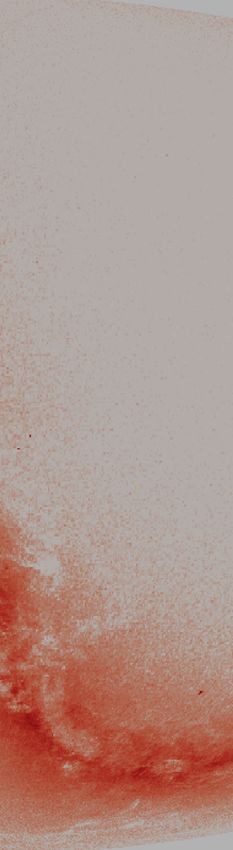
EZmock catalogues for eBOSS DR16                               1153
simulations. However, due to the inaccuracy of ZA in the nonlinear             distribution function (PDF) of the tracers by a power-law relation:
regime, the analytical form of B is not enough for a precise bias
                                                                               P (nt ) = Abnt ,                                                         (18)
model. The actual ρ t is generated with a rank ordering process
detailed in Section 2.2.4, in a numerical manner.                              where P(nt ) denotes the probability of having a cell with nt tracers,
   In this section, we focus on the deterministic part of the analytical       and b and A are two free parameters, with the restrictions A > 0 and
bias description. To form gravitational bound systems, such as dark            0 < b < 1. This serves as an additional effective bias description.
matter haloes, a minimum local density is required to overcome the                Moreover, since we aim at generating mock catalogues with
background expansion (e.g. Percival 2005). This density threshold              desired number densities in the cubic volume (see equations (4)–
is crucial for the correct modelling of the three-point statistics of          (6)), the expected total number of tracers Nttot is given, which can

                                                                                                                                                                Downloaded from https://academic.oup.com/mnras/article/503/1/1149/6149160 by University of Portsmouth Library user on 18 May 2021
dark matter haloes (Kitaura et al. 2015). Thus, we introduce a critical        also be expressed by
density ρ c , and add a term θ (ρ m − ρ c ) to the bias function, where θ

                                                                                         nt,max
denotes the step function:                                                     Nttot =            nc (nt ) · nt ,                                       (19)

           0, x < 0;                                                                     nt =1
θ (x) =                                                              (14)
           1, x ≥ 0.                                                           with
   Apart from the density threshold, Chuang et al. (2015a) applies             nc (nt ) = Ncell P (nt ) ,                                               (20)
also a density saturation, i.e. regions with densities above the
saturation ρ sat are treated equally for the stochastic generation of          nt,max = minnt >0 {nt | Ncell P (nt ) < 0.5} .                           (21)
haloes. This saturation is responsible for the amplitude of the power
spectrum of the resulting tracers. Besides, Neyrinck et al. (2014)             Here, nc (nt ) indicates the number of cells containing nt tracers, Ncell
finds an exponential cut-off of the halo bias relation:                        indicates the total number of cells (10243 in this work), nt, max is the
                                                                               maximum expected number of tracers per grid cell, and the operator
ρh ∝ ρmα exp (ρm /ρexp )− .                                            (15)      · denotes the nearest integer. Thus, there is only one degree-of-
For simplicity, we account for both effects with the following form            freedom for the PDF model. So we treat only the base b as a free
(Baumgarten & Chuang 2018):                                                    parameter.
                                                                                  We then map nc (nt ) to the expected tracer number density ρ t ,
ρt = θ(ρm − ρc ) ρsat [1 − exp (−ρm /ρexp )] Bs ,                      (16)    which is estimated by the bias relations described in the previous
where Bs denotes the stochastic bias term, which serves as a                   sections, in descending order. For instance, we rank the cells by ρ t ,
random rescaling factor of the deterministic biased density field.             and assign nt, max tracers to nc (nt, max ) cells with the highest ρ t values,
Moreover, since there are strong degeneracies between ρ sat and other          and then (nt, max − 1) tracers to the next nc (nt, max − 1) cells, etc.
parameters, we fix ρ sat = 10 in practice.                                     Thus, the exact values of ρ t defined in equation (16) is irrelevant for
                                                                               our purpose, as they are effectively modified based on their orders.
                                                                                  The tracers are then assigned randomly to the dark matter particles
2.2.3 Stochastic bias relations                                                in each grid cell, if there are any. For cells without enough number of
                                                                               dark matter particles, we randomly pick a position in the cell for the
We introduce a scatter to the bias relation to account for the
                                                                               tracer, which potentially damps the BAO feature. However, this effect
stochasticity of tracers, i.e. (Chuang et al. 2015a)
                                                                              is subdominant in this work, as the fractions of LRGs, ELGs, and
        1 + G(λ), G(λ) ≥ 0;                                                    QSOs that are randomly placed, are only ∼ 6 per cent, 16 per cent,
Bs =                                                      (17)
        exp(G(λ)), G(λ) < 0.                                                   and 4 per cent respectively. Moreover, the strength of the BAO
Here, G(λ) indicates a random number drawn from a Gaussian                     feature has little impacts on the covariance matrices, compared to the
distribution centred at 0, and with the standard deviation λ. In               contribution of the broad-band amplitudes. Thus, the enhancement of
particular, the exponential function is for avoiding negative bias             the BAO feature in the input power spectrum introduced by Chuang
values.                                                                        et al. (2015a), for correcting the BAO smearing due to the smooth
   In general, the stochastic bias of galaxies is non-Poissonian and           galaxy distribution inside grid cells, is no longer necessary.
depends on the environments (Somerville et al. 2001; Casas-Miranda
et al. 2002). Nevertheless, it is the order of tracer densities in different   2.2.5 Redshift space distortions
cells that matters in this work, rather than the actual functional form
for the scatter. This is because the densities are further modified            The linear peculiar velocity field in the ZA is (see e.g. Bernardeau
by rank ordering with a PDF mapping scheme detailed in the next                et al. 2002)
subsection. For a more realistic description of stochastic biases, see         uZA (q, a) = af (a)H (a) ZA (q, a),                                     (22)
the negative binomial distribution proposed by Kitaura et al. (2014),
and further validated in Vakili et al. (2017); Pellejero-Ibañez et al.        where f(a) is the dimensionless linear growth rate:
(2020).                                                                                  d ln D1 (a)
   In practice, the value of λ in equation (17) alters mainly the              f (a) =               .                                             (23)
                                                                                           d ln a
amplitude of the power spectrum and bispectrum, and the same effect
can be achieved by the other parameters, such as ρ c and ρ exp , hence         In the linear regime of gravitational instability, galaxy velocities are
we set λ = 10 throughout this work.                                            unbiased, i.e. they follow faithfully dark matter velocities (Hamilton
                                                                               1998). To account for the random motion of individual tracers with
                                                                               respect to the bulk flow of dark matter, we further introduce an
2.2.4 PDF mapping scheme                                                       isotropic 3D Gaussian motion to the linear coherent velocity field,
                                                                               for the modelling of tracer peculiar velocities ut :
To further correct the tracer number density ρ t , and map it to
the number of tracers per grid cell nt , we model the probability              ut = uZA + G(ν),                                                         (24)

                                                                                                                      MNRAS 503, 1149–1173 (2021)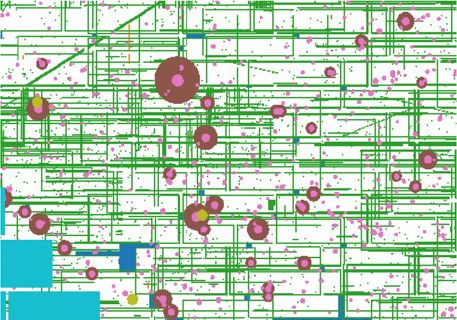
1154         C. Zhao et al.
Table 1. A list of the parameters for the effective bias modelling of EZmock.   (SUGAR; Rodrı́guez-Torres et al. 2016) used for BOSS DR12 Patchy
                                                                                mocks (Kitaura et al. 2016).
Parameter            Equation                  Description            Value

ρc                         (16)               Critical density         Free
ρ sat                      (16)             Density saturation          10      2.3.1 Coordinate conversion
ρ exp                      (16)            Density modification        Free
                                                                                Taking into account the periodic boundary conditions, we firstly
λ                          (17)               Stochastic bias           10
b                          (18)            Base of PDF mapping         Free     remap the (5 h−1 Gpc)  √
                                                                                                          3
                                                                                                              EZmock
                                                                                                                 √ box into a cuboid, with the side
ν                          (24)            Random local motion         Free     lengths being 5, 5 2, and 5/ 2 h−1 Gpc, respectively. The cuboid

                                                                                                                                                           Downloaded from https://academic.oup.com/mnras/article/503/1/1149/6149160 by University of Portsmouth Library user on 18 May 2021
                                                                                is then shifted and rotated without rescaling, such that all eBOSS
                                                                                DR16 tracers can be covered by it. To this end, the translation and
where G(ν) denotes a random vector drawn from an isotropic 3D                   rotation parameters are determined by comparing the cuboid with the
Gaussian distribution centred at 0, and with the standard deviation             eBOSS tracers in comoving coordinates, with the observer placed at
ν (in km s−1 ). This is essentially a modelling of the Maxwellian               the origin. Here, equatorial coordinates (RA, dec) and redshift z of
peculiar velocity distribution. Another formula for the local random            the eBOSS data are transformed to Cartesian comoving coordinates
velocities commonly used is the exponential distribution, but we did            (xc , yc , zc ) following
not test it since the Gaussian distribution has given already reasonable               z
agreements within the scales we are interested in, in terms of the              rc = 0 √ c dz                 ,                                 (25)
                                                                                          H0    +m (1+z )3
redshift-space clustering statistics. In general, the random motion
accounts only for small-scale clustering measurements, i.e. 2PCF                xc = rc cos (dec) cos (RA),                                        (26)
monopole and quadrupole on scales smaller than 10 and 50 h−1 Mpc
respectively. Furthermore, the effects are more obvious for Fourier-            yc = rc cos (dec) sin (RA),                                        (27)
space clustering, at k  0.1 h Mpc−1 .
                                                                                zc = rc sin (dec),                                                 (28)

2.2.6 Summary of model parameters                                               where rc denotes the radial comoving distance, and H0 =
                                                                                100 h km s−1 Mpc−1 is the Hubble parameter at z = 0.
So far we have introduced six EZmock parameters for the effective                  Furthermore, we have ensured that there is enough space between
modelling of tracer biases, and they are summarized in Table 1.                 the surface of the cuboid and the boundaries of the survey volume
Since some of the parameters are highly correlated, and we fix the              in comoving space, for preserving a complete mock sample inside
density saturation ρ sat and the width λ of the Gaussian random                 the survey volume in redshift space, in which the redshifts of
distribution for the stochastic biasing. Thus, there are four free              tracers are modified by their radial peculiar velocities (Harrison
parameters to be calibrated with the two- and three-point clustering            1974):
statistics of the reference catalogues, i.e. the BOSS DR12 CMASS
and eBOSS DR16 catalogues. In order to take into account the impact             zs = zr + (ut · r̂ c )(1 + zr )/c.                                 (29)
of survey geometry on the clustering statistics, we calibrate these free        Here, zr and zs are the redshifts of tracers in real and redshift space
parameters only with the EZmock light-cone catalogues that mimic                respectively, r̂ c denotes the unit line-of-sight vector in comoving
the geometry of eBOSS DR16 data.                                                space, and the peculiar velocity ut is described in Section 2.2.5.
   Since the observational systematics affect mainly scales outside             In particular, zr is obtained by applying the inverse transformation
the range of clustering statistics for EZmock calibrations (see                 of equations (25)–(28) to all the mock tracers, together with their
Section 2.5 for scales relevant for the calibration, and Section 3              equatorial coordinates. Note that equation (29) is slightly different
for the comparison between complete and realistic mocks), and it is             from the original implementation of MAKE SURVEY, which uses a
relatively computational expensive to apply observational effects to            single value of zr for all the mock tracers in the cuboid for the
the mock catalogues, we calibrate the EZmock parameters with the                redshift due to peculiar velocities.
complete set of EZmock light-cones, rather than the realistic ones.
In practice, the calibration is done with a single mock realization
by manually fine-tuning. The results are then validated using 50
                                                                                2.3.2 Survey volume trimming
realizations to eliminate impacts of cosmic variances, before the
mass production.                                                                To mimic the angular area of the BOSS DR12 CMASS and eBOSS
                                                                                DR16 data, we trim the EZmock catalogues with the BOSS/eBOSS
                                                                                footprints, which are defined by groups of sectors – regions covered
2.3 Complete light-cone catalogue construction                                  by a unique set of plates (Ross et al. 2020) – in the MANGLE polygon
To construct practical mock catalogues, various geometrical features            format. To have reliable clustering measurements, the sectors are
of the observed data have to be applied to the cubic mocks. To this             further selected according to the associate CeBOSS and Cz values –
end, we use the MAKE SURVEY6 toolkit (White et al. 2014) to rotate              CeBOSS > 0.5 and Cz > 0.5 for LRGs and QSOs, and CeBOSS ≥ 0.5
the cubic EZmock catalogues, map the tracers with observational co-             and Cz ≥ 0 for ELGs – where CeBOSS denotes the fraction of targets
ordinates, and trim the catalogues according to the survey footprints           that are assigned fibres, or without fibres only due to fibre-collision,
and veto masks defined by MANGLE7 (Swanson et al. 2008) polygon                 and Cz indicates the proportion of valid tracers with fibres, for which
files. This procedure is similar to that of the SUrvey GenerAtoR code           a reliable redshift is obtained (see Ross et al. 2020; Raichoor et al.
                                                                                2021, for more details).
                                                                                   In the radial direction, we simply select EZmock tracers with
6 https://github.com/mockFactory/make      survey                               redshifts inside the redshift range of the corresponding BOSS/eBOSS
7 https://space.mit.edu/   molly/mangle/                                        data catalogues (see equations (1) – (3)). The comoving volume of

MNRAS 503, 1149–1173 (2021)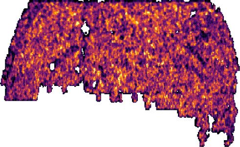
EZmock catalogues for eBOSS DR16 1155
Downloaded from https://academic.oup.com/mnras/article/503/1/1149/6149160 by University of Portsmouth Library user on 18 May 2021
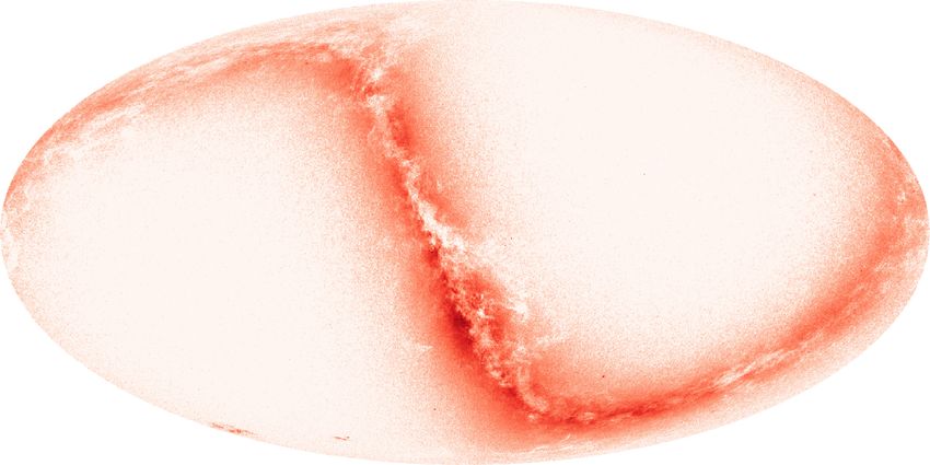
Figure 3. The comoving volume of EZmock catalogues after survey volume trimming, compared with the (5 h−1 Gpc)3 periodic box for constructing the
mocks. Regions with different colours indicate the redshift slices used for reproducing the redshift evolution of clustering statistics (see Section 2.3.5). The QSO
sample in the NGC benefits from the periodic boundary conditions, as its comoving volume is too large to be placed inside the box.
shapes and distributions of these masks depend on the brightness of
the tracers, sources of the images, and the calibration process. The
angular veto masks of the eBOSS DR16 and BOSS DR12 samples
are shown in Fig. 4, where the colours indicate different types of
masks, i.e. regions removed for different reasons (see Ross et al.
2020; Raichoor et al. 2021, for more details).
In practice, the LRG and QSO veto masks are encoded as MANGLE
polygons, and can be simply applied with the MPLY TRIM tool of
the MAKE SURVEY package. However, as can be seen in Fig. 4, the
eBOSS ELG veto masks are much more complicated than those of
the other tracers. Thus, it is not practical to translate the ELG masks
to simple polygons. Instead, the mask information is associated with
each pixel of the DECaLS bricks (Raichoor et al. 2021). We then
use the BRICKMASK9 code to apply the ELG masks, which is made
publicly available.
2.3.4 Radial selection and FKP weighting
To replicate the radial number densities n(z) of BOSS/eBOSS tracers,
we randomly discard mock objects at a given redshift with the
probability
ndata (z)
Figure 4. Angular veto masks for eBOSS DR16 tracers and BOSS DR12 Pdiscard (z) = 1 − , (30)
CMASS LRGs, for the same patch of the sky. Tracers in the coloured regions nbox
mock
are removed for various reasons, such as bright source contaminations or
where ndata indicates the radial comoving number density distribution
unreliable photometric measurements.
of the observed data, which is rescaled to the cosmology for the
the EZmock catalogues after survey volume trimming, compared to EZmock construction (m = 0.307115), and nbox mock denotes the
the original cubic periodic boxes, are shown in Fig. 3.8 number density of mock tracers in periodic boxes (see equations (4)–
(6) and Fig. 2). In particular, ndata (z) and Pdiscard (z) are evaluated for
different subsamples separately, i.e. the two Galactic caps. Moreover,
2.3.3 Veto masks since the ELG data is further split into four chunks10 – eboss23
and eboss25 for NGC, eboss21 and eboss22 for SGC – due
Inside the survey volume there are still angular patches to be removed, to their different spectroscopic properties (Raichoor et al. 2021),
such as fields that were not observed, or regions that are too close to
bright object to have reliable redshift measurements. In general, the
9 https://github.com/cheng-zhao/brickmask
10 ‘Chunks’ are regions in which the plate and fibre assignments are performed
8 The corresponding 3D illustrations are available at https://skfb.ly/6TRz9 independently.
MNRAS 503, 1149–1173 (2021)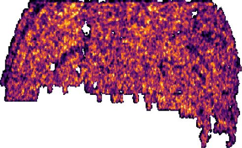
1156         C. Zhao et al.
                                                                               for LRGs (including CMASS), ELGs, and QSOs, respectively.
                                                                               They broadly correspond to the power spectrum amplitude at
                                                                               k ∼ 0.1 h Mpc−1 , for the different tracers.

                                                                               2.3.5 Redshift slices
                                                                               With the FKP weights evaluated, the complete EZmock catalogues
                                                                               are ready for clustering measurements. However, since the cubic

                                                                                                                                                              Downloaded from https://academic.oup.com/mnras/article/503/1/1149/6149160 by University of Portsmouth Library user on 18 May 2021
                                                                               mock catalogues are constructed at a specific redshift, the redshift
                                                                               evolution of structure growth, galaxy bias, and peculiar motion are
                                                                               not taken into account. To be more accurate, we construct the EZmock
                                                                               catalogues in several redshift slices, with the cubic mocks generated
                                                                               at the effective redshift zeff inside the bins. In particular, the effective
                                                                               redshift is measured from the data catalogues, with the definition
                                                                               (Samushia et al. 2014)

                                                                                (j )

                                                                                         Ndata
                                                                                                     j

                                                                                                               Ndata

                                                                               zeff =          (wi2 zi )             wi2 , j = 1, 2,                   (35)
                                                                                           i                     i
                                                                                    zlow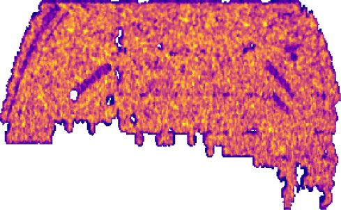
EZmock catalogues for eBOSS DR16                          1157
Table 2. The final redshift slices for the production of EZmock catalogues,       we keep only the angular positions of these random catalogues, and
with the corresponding effective redshift (equation (35)) and (weighted)          randomly assign the shuffled redshifts of the EZmock catalogues
number of tracers from the observed data. Ndata denotes the number of objects     to the angular random positions, to create the ‘shuffled’ random
in each redshift bin, and w i indicates the total photometric and spectroscopic   catalogues. Note that there is one ‘shuffled’ random catalogue for
systematic weights.
                                                                                  each of the EZmock realizations. The consequences of the two sets
                                                                      N
                                                                                  of random catalogues are shown in Section 3.
                                                                       data
                                                  (2)
Sample            zlow    zhigh      zeff        zeff       Ndata           wi
                                                                        i

CMASS LRG         0.6      0.65     0.626       0.392     114441     122385       2.5 EZmock parameter calibration

                                                                                                                                                              Downloaded from https://academic.oup.com/mnras/article/503/1/1149/6149160 by University of Portsmouth Library user on 18 May 2021
                  0.65     0.7      0.675       0.455      57561     61461.9      We aim at encoding redshift evolution in the EZmock light-cone
                  0.7      0.8      0.737       0.545      30899     33024.2
                                                                                  catalogues. To this end, besides constructing mocks at different
                  0.8      1.0      0.847       0.719       2473      2643.8
                                                                                  effective redshifts, the effective bias model of EZmock has to be
eBOSS LRG         0.6      0.65     0.625       0.391       28152    29983.1      adjusted for each of the redshift slices. This requires individual
                  0.65     0.7      0.675       0.456       33557    35828.4      calibrations of EZmock parameters (see Table 1) for each bin, with
                  0.7      0.8      0.751       0.564       64460    68592.7
                                                                                  the clustering of observed data catalogues measured in corresponding
                  0.8      0.9      0.847       0.719       37080    39099.7
                  0.9      1.0      0.940       0.885       11567    12130.2
                                                                                  redshift ranges. However, for many of the redshift bins listed in
                                                                                  Table 2, the number of tracers are too low for precise measurements
eBOSS ELG         0.6      0.7      0.658       0.434       10046    11667.4      of two- and three-point statistics from the observational data, and the
                  0.7      0.75     0.725       0.526       20275    23373.6
                                                                                  calibration results may be dominated by statistical noise.
                  0.75     0.8      0.775       0.601       33487    38857.9
                  0.8      0.85     0.825       0.682       34631    40140.4
                                                                                     To circumvent this problem, we use larger but overlapping redshift
                  0.85     0.9      0.876       0.767       27831    32231.0      bins to determine the EZmock parameters, as shown in Table 2.
                  0.9      1.0      0.950       0.903       32721    37792.2      When calibrating EZmock parameters for each bin, we compare the
                  1.0      1.1      1.047       1.097       14745    16997.8      following clustering statistics measured from the complete EZmock
eBOSS QSO         0.8      1.0      0.907       0.826       35988    38026.4
                                                                                  light-cone catalogues for both NGC and SGC, with the ones obtained
                  1.0      1.2      1.104       1.223       47025    50276.2      from BOSS/eBOSS data:
                  1.2      1.4      1.301       1.697       57120    61230.1
                                                                                     (i) ξ 0 (s), ξ 2 (s): 2PCF monopole and quadrupole, with the galaxy
                  1.4      1.6      1.500       2.252       55758    59573.2
                                                                                  pair separation range of s ∈ [10, 50] h−1 Mpc.
                  1.6      1.8      1.700       2.894       56678    60640.0
                  1.8      2.0      1.898       3.606       50774    54310.4         (ii) P0 (k), P2 (k): power spectrum monopole and quadrupole,
                  2.0      2.2      2.094       4.389       40357    42731.2      with the Fourier mode range of k ∈ [0.1, 0.3] h Mpc−1 (apart from
                                                                                  eBOSS QSO NGC, which is only calibrated on scales up to
                                                                                  k ∼ 0.24 h Mpc−1 , see Section 3.3.1).
                                                                                     (iii) B(k1 , k2 , θ 12 ): bispectrum, with k1 = 0.1 ± 0.01 h Mpc−1 ,
2.4 Random catalogue creation                                                     k2 = 0.05 ± 0.01 h Mpc−1 , and θ 12 being the angle between k1 and
In order to account for the survey window function, including the                 k2 .
radial number density of tracers, random catalogues are required
                                                                                    In particular, the ranges of the two-point statistics are chosen to
for clustering measurements. One simple way to generate random
                                                                                  be nonsensitive to observational systematic effects, and the same
catalogue for EZmock catalogues is to apply the light-cone catalogue
                                                                                  EZmock parameters are used for the two Galactic caps.
creation procedure described in Section 2.3 (except the redshift
                                                                                    Then, we use a similar way as in Ata et al. (2018), to model the
division in Section 2.3.5, as there is no evolution for a random
                                                                                  redshift evolution of the parameters, i.e.
catalogue), to a uniform random sample in comoving space. In this
                                                                                            (2)                              (2)
case, a single random catalogue is necessary for each type of the                 p(zeff , zeff ) = c0,p + c1,p zeff + c2,p zeff ,                    (36)
tracers in individual Galactic caps.
   However, the radial selection function of the BOSS DR12 CMASS                  where the coefficients c0, p , c1, p , and c2, p are obtained from linear
and eBOSS DR16 catalogues are not directly sampled from the                       regressions with the redshift bins shown in Table 3, for the EZmock
number density of data. Instead, redshifts of the observed data are               parameter p. This relationship is applied to all the redshift slices
shuffled, and randomly assigned to the angular random catalogues                  listed in Table 2, to infer the EZmock parameters for the fine bins.
(Reid et al. 2016; Ross et al. 2020; Raichoor et al. 2021). This is               For parameters that do not vary much with redshift, we use only
because the true redshift distribution of data is usually complicated             a fixed value for all redshift slices. Finally, we examine the fitting
and unknown, since it depends on various imaging and spectroscopic                results with 50 EZmock realizations, and fine tune the parameters
effects. Indeed, the comoving number density shown in Fig. 2 is only              if necessary. The resulting EZmock parameters for different redshift
a binned estimation of the true radial selection function, whereas, the           slices are shown in Table 4.
shuffled approach ensures the correct radial distribution of random
objects automatically. Nevertheless, this method introduces a radial
                                                                                  2.6 Observational effects
effect that is similar to an additional window function, and bias the
clustering measurements on large scales significantly (de Mattia &                The complete set of EZmock catalogues do not present the inhomo-
Ruhlmann-Kleider 2019). To investigate this problem, we create also               geneity of the angular distribution of tracers due to various observa-
random catalogues for the mocks with the shuffled method.                         tional effects, e.g. the quality of photometric and spectroscopic data.
   In practice, we generate firstly the random catalogue with redshifts           These effects are typically treated as systematics, and are (partially)
sampled from the spline interpolation of the comoving number                      corrected by imaging and spectroscopic weights (e.g. Ross et al.
density measured from the BOSS/eBOSS data, as is done in Sec-                     2020; Raichoor et al. 2021). To account for their impacts on the
tion 2.3.4. And we dub them the ‘sampled’ random catalogues. Then,                covariance matrices for clustering measurements, we generate more

                                                                                                                           MNRAS 503, 1149–1173 (2021)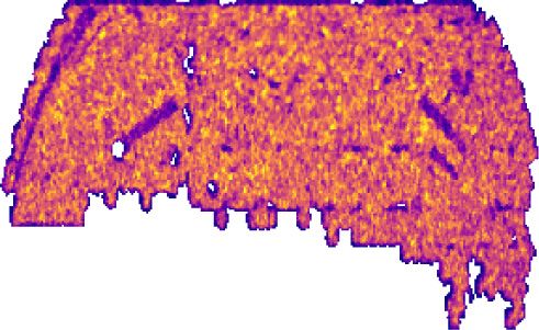
1158         C. Zhao et al.
Table 3. The redshift slices used for the calibration of EZmock catalogues,        eBOSS ELG target selection is not homogenous inside eBOSS
with the corresponding effective redshift (equation (35)) and (weighted)           chunks, especially for eboss23, resulting in an imaging depth
number of tracers from the observed data. Ndata denotes the number of objects      dependent number density of ELGs (Raichoor et al. 2017). This
in each redshift bin, and w i indicates the total photometric and spectroscopic    effect is migrated to the EZmock catalogues by the same strategy
systematic weights.
                                                                                   for generating the random catalogues for the observed data (see
                                                                       N
                                                                                   Raichoor et al. 2021). Basically the g-, r-, and z-band imaging depths
                                                                        data
                                                   (2)
Sample            zlow    zhigh       zeff        zeff       Ndata           wi    are combined linearly, and the radial number densities of ELGs are
                                                                         i
                                                                                   evaluated inside three quantiles of the combined depth, for each
CMASS LRG        0.6      0.7        0.652        0.426     172002     183847      eBOSS chunk. The EZmock ELGs are then split into the quantiles,

                                                                                                                                                               Downloaded from https://academic.oup.com/mnras/article/503/1/1149/6149160 by University of Portsmouth Library user on 18 May 2021
                 0.65     0.75       0.696        0.485      81206     86695.2     and applied radial selections separately. In this case, the actual radial
                 0.7      0.8        0.737        0.545      30899     33024.2     density of ELGs is anisotropic, and cannot be described by a simple
                 0.75     1.0        0.791        0.628       9727     10434.8     redshift-dependent function. Consequently, the random catalogues
eBOSS LRG        0.6      0.7        0.652        0.426      61709     65811.5     for the realistic ELG EZmock catalogues are generated using the
                 0.65     0.8        0.727        0.531      98017     104421      ‘shuffled’ scheme, by taking redshifts of galaxies in the quantiles
                 0.7      0.9        0.797        0.638     101540     107692      separately.
                 0.8      1.0        0.878        0.773      48647     51229.9
eBOSS ELG        0.6      0.8        0.714        0.512      63808     73898.9
                 0.7      0.9        0.805        0.651     116224     134603      2.6.2 Angular photometric systematics
                 0.8      1.0        0.905        0.821      95183     110164
                 0.9      1.1        0.994        0.991      47466      54790      Anisotropic effects that the photometric process carries, such as
eBOSS QSO        0.8      1.3        1.077        1.181     110950     118238      stellar density, Galactic extinction, seeing, and imaging depth, are
                 1.1      1.5        1.305        1.717     110326     118197      correlated with the angular distributions of the samples for large-
                 1.3      1.7        1.499        2.262     113477     121358      scale analysis (e.g. Ross et al. 2017; Xavier et al. 2019). To mimic
                 1.5      1.9        1.699        2.899     110370     117993      these effects in EZmock catalogues, we extract an angular map of
                 1.7      2.2        1.930        3.747      65077     69150.3     the photometric properties from the imaging sample, and randomly
                                                                                   discarding mock tracers with the probability following this map.
Table 4. The calibrated EZmock parameters for different redshift slices, that      For LRGs and QSOs, the map is generated by linear regressions
are used for both NGC and SGC.                                                     for different photometric effects (Ross et al. 2020), while for ELGs
                                                                                   we use directly a smoothed angular target density map of the data,
Sample             zlow      zhigh           ρc     ρ exp        b             ν   with a beam size of 1 deg (de Mattia et al. 2021). The corrections
                                                                                   are then done by adding photometric weights to the mocks, which
CMASS LRG         0.6        0.65        0.90       2.80      0.240          175
                                                                                   are estimated by linear regressions to the angular completeness (see
                  0.65       0.7         1.14       3.84      0.249          175
                  0.7        0.8         1.37       4.19      0.252          175
                                                                                   Ross et al. 2020; Raichoor et al. 2021, for details) for each mock
                  0.8        1.0         1.55       3.88      0.251          175   realization individually, thus allowing stochasticity for the systematic
                                                                                   weights.
eBOSS LRG         0.6        0.65        0.35       2.50      0.180          190
                  0.65       0.7         0.63       3.46      0.205          190
                  0.7        0.8         0.80       3.00      0.220          190
                  0.8        0.9         1.05       3.79      0.257          190   2.6.3 Fibre collision
                  0.9        1.0         0.93       4.40      0.295          190
                                                                                   Due to the finite size of optical fibres, the spectra of two tar-
eBOSS ELG         0.6        0.7         0.50       1.00      0.181          150   gets with the angular separation less than 62 arcsec cannot be
                  0.7        0.75        0.50       1.00      0.180          150
                                                                                   both measured with one plate. Thus, one of the targets has to
                  0.75       0.8         0.50       1.00      0.186          150
                  0.8        0.85        0.50       1.00      0.195          150
                                                                                   be rejected if they do not reside in sectors covered by different
                  0.85       0.9         0.50       1.00      0.211          150   plates.
                  0.9        1.0         0.50       1.00      0.243          150      We use the angular friends-of-friends (FoF) algorithm provided
                  1.0        1.1         0.50       1.00      0.300          150   in the NBODYKIT11 (Hand et al. 2018) package, to detect groups of
eBOSS QSO         0.8        1.0         1.00       0.47      0.0100         200
                                                                                   EZmock tracers that are in collision, and mark objects to be removed.
                  1.0        1.2         0.88       0.66      0.0089         217   Then, the groups are distributed to the sectors of the observational
                  1.2        1.4         0.57       0.81      0.0057         330   data, and some of the collisions can be resolved when the objects are
                  1.4        1.6         0.41       0.92      0.0033         415   in sectors belonging to multiple plates.
                  1.6        1.8         0.37       0.99      0.0017         474      To correct the clustering statistics with fibre collision, remaining
                  1.8        2.0         0.49       1.02      0.0010         501   mock tracers in collision groups are up-weighted by the ratio
                  2.0        2.2         0.74       1.01      0.0011         501   between the original number of targets, and the number of assigned
                                                                                   fibres, for each of the groups (cf. Hou et al. 2021, for more
realistic EZmock catalogues by introducing observational effects to                investigations on the fibre collision weights). The fibre collision
the complete mocks for eBOSS DR16 tracers.                                         effects on the configuration space measurements can be further sup-
                                                                                   pressed by the pairwise-inverse-probability (PIP) weighting scheme,
                                                                                   which is an unbiased procedure for all scales (Mohammad et al.
2.6.1 Depth dependent radial density                                               2020).
For the eBOSS ELG EZmock catalogues, we start from the complete
realizations before applying radial selection (see Section 2.3.4).
This is because the imaging depth of the DECaLS data used for                      11 https://github.com/bccp/nbodykit

MNRAS 503, 1149–1173 (2021)
EZmock catalogues for eBOSS DR16 1159
2.6.4 Redshift failure Table 5. A list of notations for different EZmock samples.
Reliable redshifts are not always obtained from the spectra in Notation Description
practice. The redshift failure rate ffail for the eBOSS data are modelled
by regressions with the signal-to-noise ratio of the spectra, as well EZmock comp. Complete mocks with ‘sampled’ randoms: no
as IDs and positions on the focal plane of optical fibres (Ross et al. observational systematics, and redshifts of the
2020; Raichoor et al. 2021). This effect is introduced to the EZmock random catalogues are sampled from the spline
interpolation of the n(z) of observational data.
catalogues with a similar approach for eBOSS DR14 LRG QPM
EZmock R-shuf. Complete mocks with ‘shuffled’ randoms: no
mocks (Bautista et al. 2018). We associate EZmock objects with the observational systematics, and redshifts of the
Downloaded from https://academic.oup.com/mnras/article/503/1/1149/6149160 by University of Portsmouth Library user on 18 May 2021
fibre of the closest valid eBOSS tracer, and randomly down-sample random catalogues are taken randomly from the
mocks according to the modelled redshift failure rate of the data. corresponding data catalogues.
We then use the same procedure as with the data to fit our model EZmock syst. Realistic mocks with ‘shuffled’ randoms: all known
for ffail for each individual mock, and the remained mock tracers are observational systematics are applied to the data and
up-weighted by 1/(1 − ffail ). random catalogues, and redshifts of the random
catalogues are taken randomly from the
corresponding data catalogues.
3 R E S U LT S : S TAT I S T I C A L C O M PA R I S O N
B E T W E E N E Z M O C K C ATA L O G U E S A N D
B O S S / E B O S S DATA Reid et al. 2016; Ross et al. 2020) are not considered by the weights.
Thus, there can be discrepancies on the actual weighted radial
We generate 1000 realizations of EZmock catalogues, for each of counts between data and the corresponding mocks. This can be
the dataset, i.e. BOSS DR12 CMASS LRG, and eBOSS DR16 seen in Fig. 5, where the comparisons between EZmock tracers and
LRG/ELG/QSO. Thus, 46,000 EZmock boxes are generated, with BOSS/eBOSS data are shown, in terms of the (weighted) number of
the side length of 5 h−1 Gpc, for the 23 redshift slices listed in Table 2, objects at different redshifts.
and both northern and southern Galactic caps. The number of tracers For the eBOSS samples, the number of targets without fibres is
for each of the LRG, ELG, and QSO boxes are 4 × 10⁷ , 8 × 10⁷ , about 3.4 per cent of the total weighted number of LRGs, and the
and 3 × 10⁶ , respectively. It takes ∼1 million CPU hours in total, to fractions are 0.9 and 2.3 per cent for ELGs and QSOs respectively.
generate the complete set of EZmock mock light-cone catalogues, on These numbers are consistent with the mismatch between EZmock
the Cori Haswell nodes of the National Energy Research Scientifc catalogues and eBOSS data illustrated in Fig. 5. This effect is due
Computing Center (NERSC).12 The EZMOCK code is parallelized to the definition of the effective area for measuring ndata , and for
with OpenMP, and multiple realizations are run simultaneously with sectors with C(e)BOSS = 1, the radial comoving number density of
the JOBFORK13 tool, which distributes serial or OpenMP based jobs tracers from the mocks and data are still consistent (see Appendix A
to multiple computing nodes using MPI. for more discussions).
In this section, we present various statistical properties of To have accurate estimates of the clustering covariance matrices,
the EZmock catalogues and compare them with those from the it is necessary to reproduce faithfully the sample size of the
BOSS/eBOSS data. In particular, results of both the complete and observational data. Hence, the effect of CeBOSS is considered
realistic mocks are shown. Moreover, we measure the clustering in the realistic EZmock catalogues. Moreover, after including
statistics for the complete mocks with both the ‘sampled’ and both photometric and spectroscopic effects (see Section 2.6),
‘shuffled’ random catalogues, and the results are denoted by ‘EZ- a considerable fraction of the mock tracers are removed.
mock comp.’ and ‘EZmock R-shuf.’, respectively. While results Consequently, the number of objects in the mocks and data become
for the realistic mocks are always obtained using the ‘shuffled’ more comparable, though they are still not identical, since the
random catalogues (denoted by ‘EZmock syst.’). Note however small-scale clustering of EZmock catalogues does not allow precise
that the realistic joint BOSS and eBOSS LRG samples (denoted reproduction of some of the observational systematics, such as fibre
by ‘COMB BOSS’) are constructed with the combination of the collision. Finally, the systematics of the realistic EZmock catalogues
complete CMASS LRG mocks and realistic eBOSS LRG mocks. are corrected by various weights. Thus, the weighted redshift
The meanings of these notations are summarized in Table 5. distribution of mocks and data agree well again, as shown in Fig. 5.
Note that the clustering measurements of the complete mocks are Furthermore, since the number density of the cubic EZmock ELG
used for EZmock parameter calibration (see Section 2.5), while the catalogues (6.4 × 10⁻⁴ h3 Mpc−3 ) are only slightly larger than the
covariance matrices of the realistic mocks are our final products peak density of the eBOSS data in chunk eboss22, after down-
for the data analyses. The fiducial cosmological model used for sampling with observational systematics, the density of EZmock
coordinate conversion hereafter, is flat CDM with m = 0.31 (see ELGs at z ∼ 0.8 are lower than that of the eBOSS data by at
equations (25) – (28)). most 5 per cent. We then rescale the radial selection function (see
Section 2.3.4) of ELGs in chunk eboss22, to obtain the correct
number of objects in the full sample. Since this affects only a
3.1 Spatial distribution
small number of EZmock ELGs, the consequences on the covariance
The radial distributions of the complete EZmock catalogues in matrices are sub-dominant.
comoving space follows those measured from the data with all Fig. 6 shows that angular systematic map extracted from the
photometric and systematic weights by construction (see equation eBOSS DR16 data – including all the effects discussed in Section 2.6
(30)). However, the fraction of targets without fibres (C(e)BOSS ; see – as well as the comparison of the unweighted angular tracer
density between the data and one arbitrary EZmock realization.
Note however that for better illustration, veto masks due to bad
12 https://docs.nersc.gov/systems/cori photometric calibrations are not shown for ELG SGC (cf. Raichoor
13 https://github.com/cheng-zhao/jobfork et al. 2021). The large-scale angular distribution of both data and
MNRAS 503, 1149–1173 (2021)You can also read