Euclid: Effect of sample covariance - on the number counts of galaxy clusters
←
→
Page content transcription
If your browser does not render page correctly, please read the page content below
Astronomy & Astrophysics manuscript no. PAPER                                                                                      ©ESO 2021
                                               February 18, 2021

                                                                             Euclid: Effect of sample covariance
                                                                          on the number counts of galaxy clusters ?
                                                  A. Fumagalli1,2,3?? , A. Saro1,2,3,4 , S. Borgani1,2,3,4 , T. Castro1,2,3,4 , M. Costanzi1,2,3 , P. Monaco1,2,3,4 , E. Munari3 ,
                                                      E. Sefusatti1,3,4 , A. Amara5 , N. Auricchio6 , A. Balestra7 , C. Bodendorf8 , D. Bonino9 , E. Branchini10,11,12 ,
                                                        J. Brinchmann13,14 , V. Capobianco9 , C. Carbone15 , M. Castellano12 , S. Cavuoti16,17,18 , A. Cimatti19,20 ,
                                                   R. Cledassou21,22 , C.J. Conselice23 , L. Corcione9 , A. Costille24 , M. Cropper25 , H. Degaudenzi26 , M. Douspis27 ,
                                                    F. Dubath26 , S. Dusini28 , A. Ealet29 , P. Fosalba30,31 , E. Franceschi6 , P. Franzetti15 , M. Fumana15 , B. Garilli15 ,
                                                     C. Giocoli6,32 , F. Grupp8,33 , L. Guzzo34,35,36 , S.V.H. Haugan37 , H. Hoekstra38 , W. Holmes39 , F. Hormuth40 ,
                                                      K. Jahnke41 , A. Kiessling39 , M. Kilbinger42 , T. Kitching25 , M. Kümmel33 , M. Kunz43 , H. Kurki-Suonio44 ,
arXiv:2102.08914v1 [astro-ph.CO] 17 Feb 2021

                                               R. Laureijs45 , P. B. Lilje37 , I. Lloro46 , E. Maiorano6 , O. Marggraf47 , K. Markovic39 , R. Massey48 , M. Meneghetti6,32,49 ,
                                                G. Meylan50 , L. Moscardini6,20,51 , S.M. Niemi45 , C. Padilla52 , S. Paltani26 , F. Pasian3 , K. Pedersen53 , V. Pettorino42 ,
                                               S. Pires42 , M. Poncet22 , L. Popa54 , L. Pozzetti6 , F. Raison8 , J. Rhodes39 , M. Roncarelli6,20 , E. Rossetti20 , R. Saglia8,33 ,
                                                      R. Scaramella12,55 , P. Schneider47 , A. Secroun56 , G. Seidel41 , S. Serrano30,31 , C. Sirignano28,57 , G. Sirri32 ,
                                                   A.N. Taylor58 , I. Tereno59,60 , R. Toledo-Moreo61 , E.A. Valentijn62 , L. Valenziano6,32 , Y. Wang63 , J. Weller8,33 ,
                                               G. Zamorani6 , J. Zoubian56 , M. Brescia18 , G. Congedo58 , L. Conversi64,65 , S. Mei66 , M. Moresco6,20 , and T. Vassallo33
                                                                                                (Affiliations can be found after the references)
                                                                                                          Received ???; accepted ???

                                                                                                                 ABSTRACT

                                               Aims. We investigate the contribution of shot-noise and sample variance to the uncertainty of cosmological parameter constraints inferred from
                                               cluster number counts in the context of the Euclid survey.
                                               Methods. By analysing 1000 Euclid-like light-cones, produced with the PINOCCHIO approximate method, we validate the analytical model of
                                               Hu & Kravtsov 2003 for the covariance matrix, which takes into account both sources of statistical error. Then, we use such covariance to define
                                               the likelihood function that better extracts cosmological information from cluster number counts at the level of precision that will be reached by
                                               the future Euclid photometric catalogs of galaxy clusters. We also study the impact of the cosmology dependence of the covariance matrix on the
                                               parameter constraints.
                                               Results. The analytical covariance matrix reproduces the variance measured from simulations within the 10 per cent level; such difference has
                                               no sizeable effect on the error of cosmological parameter constraints at this level of statistics. Also, we find that the Gaussian likelihood with
                                               cosmology-dependent covariance is the only model that provides an unbiased inference of cosmological parameters without underestimating the
                                               errors.
                                               Key words. galaxies: clusters: general - large-scale structure of Universe - cosmological parameters - methods: statistical

                                               1. Introduction                                                           (Ωm ) (Borgani et al. 1999; Schuecker et al. 2003; Allen et al.
                                                                                                                         2011; Pratt et al. 2019). Moreover, clusters can be observed at
                                               Galaxy clusters are the most massive gravitationally bound sys-           low redshift (out to redshift z ∼ 2), thus sampling the cosmic
                                               tems in the Universe (M ∼ 1014 – 1015 M ) and they are com-               epochs during which the effect of dark energy begins to domi-
                                               posed of dark matter for 85 per cent, hot ionized gas for 12              nate the expansion of the Universe; as such, the evolution of the
                                               per cent and stars for 3 per cent (Pratt et al. 2019). These mas-         statistical properties of galaxy clusters should allow us to place
                                               sive structures are formed by the gravitational collapse of initial       constraints on the dark energy equation of state, and then de-
                                               perturbations of the matter density field, through a hierarchical         tect possible deviations of dark energy from a simple cosmolog-
                                               process of accretion and merging of small objects into increas-           ical constant (Sartoris et al. 2012). Finally, such observables can
                                               ingly massive systems (Kravtsov & Borgani 2012). Therefore                be used to constrain neutrino masses (e.g. Costanzi et al. 2013;
                                               galaxy clusters have several properties that can be used to ob-           Mantz et al. 2015; Costanzi et al. 2019; Bocquet et al. 2019; DES
                                               tain cosmological information on the geometry and the evolution           Collaboration et al. 2020), the Gaussianity of initial conditions
                                               of the large-scale structure of the Universe (LSS). In particular,        (e.g. Sartoris et al. 2010; Mana et al. 2013) and the behavior of
                                               the abundance and spatial distribution of such objects are sen-           gravity on cosmological scales (e.g. Cataneo & Rapetti 2018;
                                               sitive to the variation of several cosmological parameters, such          Bocquet et al. 2015).
                                               as the RMS mass fluctuation of the (linear) power spectrum on
                                               8 h−1 Mpc scales (σ8 ) and the matter content of the Universe                 The main obstacle in the use of clusters as cosmological
                                                                                                                         probes lies in the proper calibration of systematic uncertainties
                                                ?                                                                        that characterize the analyses of cluster surveys. First, cluster
                                                    This paper is published on behalf of the Euclid Consortium
                                               ??
                                                    e-mail: alessandra.fumagalli@inaf.it                                 masses are not directly observed but must be inferred through
                                                                                                                                                                    Article number, page 1 of 15
A&A proofs: manuscript no. PAPER

other measurable properties of clusters, e.g. properties of their      duce N-body results with sufficient precision. By using a large
galaxy population (i.e. richness, velocity dispersion) or of the       set of LPT-based simulations, we test the accuracy of an analyt-
intracluster gas (i.g., total gas mass, temperature, pressure). The    ical model for the computation of the covariance matrix and de-
relationships between these observables and clusters masses,           fine which is the best likelihood function to optimize the extrac-
called scaling relations, provide a statistical measurement of         tion of unbiased cosmological information from cluster number
masses, but require an accurate calibration in order to correctly      counts. In addition, we also analyze the impact of the cosmolog-
relate the mass proxies with the actual cluster mass. Moreover,        ical dependence of the covariance matrix on the estimation of
scaling relations can be affected by intrinsic scatter due to the      cosmological parameters.
properties of individual clusters and baryonic physics effects,            This paper is organized as follows: in Sect. 2 we present the
that complicate the calibration process (Kravtsov & Borgani            quantities involved in the analysis, such as the mass function,
2012; Pratt et al. 2019). Other measurement errors are related to      likelihood function and covariance matrix, while in Sect. 3 we
the estimation of redshifts and the selection function (Allen et al.   describe the simulations used in this work, which are dark matter
2011). In addition, there may be theoretical systematics linked to     halo catalogs produced by the PINOCCHIO algorithm (Monaco
the modelling of the statistical errors: shot-noise, the uncertainty   et al. 2002; Munari et al. 2017). In Sect. 4 we present the analy-
due to the discrete nature of data, and sample variance, the un-       ses and the results that we obtain by studying the number counts:
certainty due to the finite size of the survey; in the case of a       in Sect. 4.1 (and in Appendix A) we validate the analytical model
“full-sky” survey, the latter takes the name of cosmic variance        for the covariance matrix, by comparing it with the matrix from
and describes the fact that we can observe a single random re-         simulations. In Sect. 4.2 we analyze the effect of the mass and
alization of the Universe (e.g. Valageas et al. 2011). Finally, the    redshift binning on the estimation of parameters, while in Sect.
analytical models describing the observed distributions, such as       4.3 we compare the effect on the parameter posteriors of different
the mass function and halo bias, have to be carefully calibrated,      likelihood models. In Sect. 5 we present our conclusions. While
to avoid introducing further systematics (e.g. Sheth & Tormen          this paper is focused on the analysis relevant for a cluster survey
2002; Tinker et al. 2008, 2010; Bocquet et al. 2015; Despali et al.    similar in sky coverage and depth to the Euclid one, for com-
2016; Castro et al. 2021).                                             pleteness we provide in Appendix B results relevant for present
     The study and the control of these uncertainties are fun-         and ongoing surveys.
damental for future surveys, which will provide large cluster
samples that will allow us to constrain cosmological parame-
ters with a level of precision much higher than that obtained so       2. Theoretical background
far. One of the main forthcoming surveys is the European Space         In this section we introduce the theoretical framework needed to
Agency (ESA) mission Euclid1 , planned for 2022, which will            model the cluster number counts and derive cosmological con-
map ∼ 15 000 deg2 of the extragalactic sky up to redshift 2, in        straints via Bayesian inference.
order to investigate the nature of dark energy, dark matter and
gravity. Galaxy clusters are among the cosmological probes that
will be used by Euclid: the mission is expected to yield a sam-        2.1. Number counts of galaxy clusters
ple of ∼ 105 clusters using photometric and spectroscopic data         The starting point to model the number counts of galaxy clusters
and through gravitational lensing (Laureijs et al. 2011; Euclid        is given by the halo mass function dn(M, z), defined as the co-
Collaboration: Adam et al. 2019). A forecast of the capability         moving volume number density of collapsed objects at redshift z
of the Euclid cluster survey has been performed by Sartoris et al.     with masses between M and M + dM (Press & Schechter 1974),
(2016), which shows the effect of the photometric selection func-
tion on the number of detected objects and the consequent cos-
mological constraints for different cosmological models. Also,         dn(M, z) ρ̄m         d ln ν
                                                                               =    ν f (ν)        ,                                     (1)
Köhlinger et al. (2015) show that the weak lensing systematics          d ln M   M          d ln M
in the mass calibration are under control for Euclid, which will       where ρ̄m /M is the inverse of the Lagrangian volume of a halo of
be limited by the cluster samples themselves.                          mass M, and ν = δc /σ(R, z) is the peak height, defined in terms
     The aim of this work is to assess the contribution of shot-       of the variance of the linear density field smoothed on scale R,
noise and sample variance to the statistical error budget expected                     Z
for the Euclid photometric survey of galaxy clusters. The ex-                       1
                                                                       σ (R, z) = 2
                                                                         2
                                                                                           dk k2 P(k, z) WR2 (k) ,                    (2)
pectation is that the level of shot-noise error would decrease                     2π
due to the large number of detected clusters, making the sam-
ple variance not negligible anymore. To quantify the contribu-         where R is the radius enclosing the mass M = 4π       3 ρ̄m R , WR (k)
                                                                                                                                    3

tion of these effects, an accurate statistical analysis is required,   is the filtering function and P(k, z) the initial matter power spec-
to be performed on a large number of realizations of past-light        trum, linearly extrapolated to redshift z. The term δc represents
cones extracted from cosmological simulations describing the           the critical linear overdensity for the spherical collapse and con-
distribution of cluster-sized halos. This is made possible using       tains a weak dependence on cosmology and redshift that can be
approximate methods for such simulations (e.g. Monaco 2016,            expressed as (Nakamura & Suto 1997)
for a review). A class of these methods describes the forma-                       3
tion process of dark matter halos, i.e. the dark matter compo-         δc (z) =      (12π)2/3 [1 + 0.012299 log10 Ωm (z)] .              (3)
nent of galaxy clusters, through Lagrangian Perturbation Theory                   20
(LPT), which provides the distribution of large-scale structures       One of the main characteristics of the mass function is that, when
in a faster and computationally less expensive way than through        expressed in terms of the peak height, its shape is nearly uni-
“exact” N-body simulations. As a disadvantage, such catalogs           versal, meaning that the multiplicity function ν f (ν) can be de-
are less accurate and have to be calibrated, in order to repro-        scribed in terms of a single variable and with the same parame-
                                                                       ters for all the redshifts and cosmological models (Sheth & Tor-
1
    http://www.euclid-ec.org                                           men 2002). A number of parametrizations have been derived by
Article number, page 2 of 15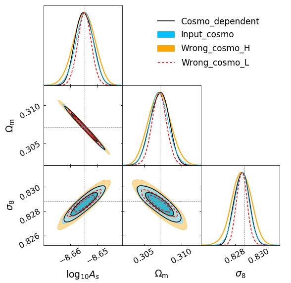
A. Fumagalli et al.: Euclid: Effect of sample covariance on the number counts of galaxy clusters

fitting the mass distribution from N-body simulations (Jenkins                 2.2. Definition of likelihood functions
et al. 2001; White 2002; Tinker et al. 2008; Watson et al. 2013),
in order to describe such universality with the highest possible               The analysis of the mass function is performed through Bayesian
accuracy. At the present time, a fully universal parametrization               inference, by maximizing a likelihood function. The posterior
has not been found yet, and the main differences between the var-              distribution is explored with a Monte Carlo Markov Chains
ious results reside in the definition of halos, which can be based             (MCMC) approach (Heavens 2009), by using a python wrapper
on the Friends-of-Friends (FoF) and Spherical Overdensity (SO)                 for the nested sampler PyMultiNest (Buchner et al. 2014).
algorithms (e.g. White 2001; Kravtsov & Borgani 2012) or on                        The likelihood commonly adopted in the literature for num-
the dynamical definition of the Splashback radius (Diemer 2017,                ber counts analyses is the Poissonian one, which takes into ac-
2020), and in the overdensity at which halos are identified. The               count only the shot-noise term. To add the sample variance con-
need to improve the accuracy and precision in the mass function                tribution, the simplest way is to use a Gaussian likelihood. In this
parametrization is reflected by the differences found in the cos-              work, we considered the following likelihood functions:
mological parameter estimation, in particular for future surveys                – Poissonian:
such as Euclid (Salvati et al. 2020; Artis et al. 2021). Another
                                                                                                Nz Y
way to predict the abundance of halos is the use of emulators,                                  Y  NM
                                                                                                      µ xiα e−µiα
built by fitting the mass function from simulations as a function                  L(x | µ) =             iα
                                                                                                                      ,                           (5)
                                                                                                α=1 i=1
                                                                                                              xiα !
of cosmology; such emulators are able to reproduce the mass
function within few percent accuracy (Heitmann et al. 2016; Mc-                   where xiα and µiα are, respectively, the observed and ex-
Clintock et al. 2019; Bocquet et al. 2020). The description of the                pected number counts in the i-th mass bin and α-th redshift
cluster mass function is further complicated by the presence of                   bin. Here the bins are not correlated, since shot-noise does
baryons, which have to be taken into account when analyzing                       not produce cross-correlation, and the likelihoods are simply
the observational data; their effect must therefore be included in                multiplied;
the calibration of the model (e.g. Cui et al. 2014; Velliscig et al.            – Gaussian with shot-noise only:
2014; Bocquet et al. 2015; Castro et al. 2021).                                                            n                      o
                                                                                                    N M exp − 1 (x − µ )2 /σ2
                                                                                                 Nz Y
     In this work, we fix the mass function assuming that the                                   Y             2 iα      iα     iα
                                                                                  L(x | µ, σ) =                                     ,       (6)
model has been correctly calibrated. The reference mass func-                                                    q
tion that we assume for our analysis is the one by (Despali et al.                              α=1 i=1            2πσ2iα
2016, hereafter D16) 2 ,
                                                                                  where σ2iα = µiα is the shot-noise variance. This function rep-
                                                                                  resents the limit of the Poissonian case for large occupancy
                                    !1/2                                          numbers;
                               ν0
                          !
                     1
                                           e−ν /2 ,
                                              0
ν f (ν) = 2A 1 +                                                         (4)    – Gaussian with shot-noise and sample variance:
                    ν0p        2π                                                                    n                          o
                                                                                                 exp − 21 (x − µ)T C −1 (x − µ)
                                                                                  L(x | µ, C) =            √                      ,           (7)
with ν0 = aν2 . The values of the parameters are: A = 0.3298,                                                2π det[C]
a = 0.7663, p = 0.2579 (“All z - Planck cosmology” case in
                                                                                   where x = {xiα } and µ = {µiα }, while C = {Cαβi j } is the
D16). Comparisons with numerical simulations show departures
                                                                                   covariance matrix which correlates different bins due to the
from the universality described by this model of the order of
                                                                                   sample variance contribution. This function is also valid in
5 − 8%, provided that halo masses are computed within the virial
                                                                                   the limit of large numbers, as the previous one.
overdensity, as predicted by the spherical collapse model.
    Besides the systematic uncertainty due to the fitting model,                   We maximise the average likelihood, defined as
the mass function is affected by two sources of statistical error                              NS
(which do not depend on the observational process): shot-noise                             1 X
                                                                               ln Ltot =          ln L(a) ,                                       (8)
and sample variance. Shot-noise is the sampling error that arises                          NS a=1
from the discrete nature of the data and contributes mainly to
the high-mass tail of the mass function, where the number of ob-               where NS = 1000 is the number of light-cones and ln L(a) is
jects is lower, being proportional to the square root of the num-              the likelihood of the a-th light-cone evaluated according to the
ber counts. On the other hand, sample variance depends only on                 equations described above. The posteriors obtained in this way
the size and the shape of the sampled volume; it arises as a con-              are consistent with those of a single light-cone but, in principle,
sequence of the existence of super-sample Fourier modes, with                  centered on the input parameter values since the effect of cos-
wavelength exceeding the survey size, that can not be sampled                  mic variance that affects each realization of the matter density
in the analyses of a finite volume survey. Sample variance in-                 field is averaged-out when combining all the 1000 light-cones;
troduces correlation between different mass and redshift ranges,               this procedure makes it easier to observe possible biases in the
unlike the shot-noise that affects only objects in the same bin.               parameter posteriors due to the presence of systematics.
For currently available data the main contribution to the error                    To estimate the differences on the parameter constraints be-
comes from shot-noise, while the sample variance term is usu-                  tween the various likelihood models, we quantify the cosmolog-
ally neglected (e.g. Mantz et al. 2015; Bocquet et al. 2019). Nev-             ical gain using the figure of merit (FoM hereafter, Albrecht et al.
ertheless, future surveys will provide catalogs with a larger num-             2006) in the Ωm – σ8 plane, defined as
ber of objects, making the sample variance comparable, or even
greater, than the shot-noise level (Hu & Kravtsov 2003).                                               1
                                                                               FoM(Ωm , σ8 ) = √                    ,                             (9)
                                                                                                det [Cov(Ωm , σ8 )]
 2
   In D16 the peak height is defined as ν = δ2c /σ2 (R, z); in such case the   where Cov(Ωm , σ8 ) is the parameter covariance matrix com-
factor “2” in Eq. (4) disappears.                                              puted from the sampled points in the parameter space. The FoM
                                                                                                                          Article number, page 3 of 15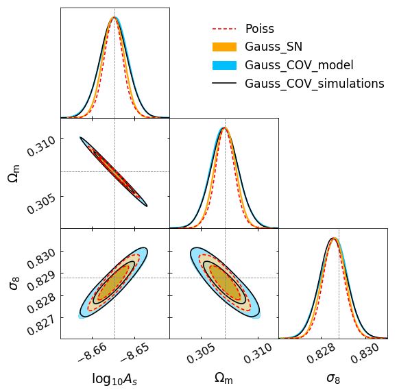
A&A proofs: manuscript no. PAPER

is proportional to the inverse of the area enclosed by the ellipse     where hNiαi and hNbiαi are respectively the expectation values
representing the 68 per cent confidence level and gives a mea-         of number counts and number counts times the halo bias in the
sure of the accuracy of the parameter estimation: the larger the       i-th mass bin and α-th redshift bin,
FoM, the more precise is the evaluation of the parameters. How-                     Z              Z
ever, a larger FoM may not indicate a more efficient method of                                dV             dn
                                                                       hNiαi = Ωsky      dz              dM     (M, z) ,          (17)
information extraction, but rather an underestimation of the error                    ∆z     dz dΩ   ∆M     dM
in the likelihood analysis.                                                           Zα            Z i
                                                                                                dV            dn
                                                                       hNbiαi = Ωsky       dz             dM     (M, z) b(M, z) , (18)
                                                                                       ∆zα    dz dΩ   ∆Mi     dM
2.3. Covariance matrix
                                                                       with Ωsky = 2π(1 − cos θ), where θ is the field-of-view angle of
The covariance matrix can be estimated from a large set of sim-        the light-cone, and b(M, z) represents the halo bias as a function
ulations through the equation                                          of mass and redshift. In the following, we adopt for the halo bias
                                                                       the expression provided by Tinker et al. (2010). The term S αβ
           1 X
               NS                                                      is the covariance of the linear density field between two redshift
Cαβi j =                          jβ − n̄ jβ ) ,
                  (n(m) − n̄iα )(n(m)                          (10)    bins,
           NS m=1 iα
                                                                                               d3 k
                                                                                            Z
                                                                       S αβ = D(zα ) D(zβ )          P(k) Wα (k) Wβ (k) ,            (19)
where m = 1, .., NS indicates the simulation, n(m)
                                                i,α is the number of                          (2π)3
objects in the i-th mass bin and in the α-th redshift bin for the m-
th catalog, while n̄i,α represents the same number averaged over       where D(z) is the linear growth rate, P(k) is the linear matter
the set of NS simulations. Such matrix describes both the shot-        power spectrum at the present time, and Wα (k) is the window
noise variance, given simply by the number counts in each bin,         function of the redshift bin, which depends on the shape of the
and the sample variance contribution, or more properly sample          volume probed. The simplest case is the spherical top-hat win-
covariance:                                                            dow function (see Appendix A), while the window function for
                                                                       a redshift slice of a light-cone is given in Costanzi et al. (2019)
                                                                       and takes the form
     j = n̄iα δαβ δi j ,
 SN
Cαβi                                                           (11)
                                                                                                   ∞   `
     j = C αβi j − C αβi j ,
 SV                  SN                                                              Z
Cαβi                                                           (12)              4π           dV X X `
                                                                       Wα (k) =           dz               (i) j` [k r(z)] Y`m (k̂) K` , (20)
                                                                                 Vα ∆zα        dz `=0 m=−`
Actually the precision matrix C −1 (which has to be included in
Eq. 7), obtained by inverting Eq. (10), is biased due to the noise     where dV/dz and Vα are respectively the volume per unit redshift
generated by the finite number of realizations; the inverse matrix     and the volume of the slice, which depend on cosmology. Also,
must therefore be corrected by a factor (Anderson 2003; Hartlap        in the above equation j` [k r(z)] are the spherical Bessel func-
et al. 2007; Taylor et al. 2013)                                       tions, Y`m (k̂) are the spherical harmonics, k̂ is the angular part
                                                                       of the wave-vector, and K` are the coefficients of the harmonic
              NS − ND − 2 −1                                           expansion, such that
 −1
Cunbiased =              C ,                                   (13)
                NS − 1
                                                                             1
                                                                       K` =  √ for ` = 0 ,
where NS is the number of catalogs and ND the dimension of the              2 π
data vector i.e. the total number of bins.
                                                                                π P`−1 (cos θ) − P`+1 (cos θ)
                                                                            r
    Although the use of simulations allows us to calculate the         K` =                                   for ` , 0 ,
covariance in a simple way, numerical estimates of the covari-                2` + 1         Ωsky
ance matrix have some limitations, mainly due to the presence
of statistical noise which can only be reduced by increasing the       where P` (cos θ) are the Legendre polynomials.
number of catalogs. In addition, simulations make it possible to
compute the matrix only at their input cosmology, preventing a         3. Simulations
fully cosmology-dependent analysis. To overcome these limita-
tions, one can adopt an analytic prescription for the covariance       The accurate estimation of the statistical uncertainty associated
matrix (Hu & Kravtsov 2003; Lacasa et al. 2018; Valageas et al.        with number counts must be carried out with a large set of simu-
2011). This involves a simplified treatment of non-linearities, so     lated catalogs, representing different realizations of the Universe.
that the validity of this approach must be demonstrated by com-        Such large number of synthetic catalogs can hardly be provided
paring it with simulations. To this end we consider the analytical     by N-body simulations, which are able to produce accurate re-
model proposed by Hu & Kravtsov (2003) and validate its pre-           sults but have high computational costs. Instead, the use of ap-
dictions against simulated data (see Sect. 4.1). As stated before,     proximate methods, based on perturbative theories, makes it pos-
the total covariance is given by the sum of the shot-noise vari-       sible to generate a large number of catalogs in a faster and far
ance and the sample covariance,                                        less computationally expensive way compared to N-body simu-
                                                                       lations. This comes at the expense of less accurate results: per-
C = C SN + C SV .                                              (14)    turbative theories give an approximate description of particle and
                                                                       halo displacements which are computed directly from the initial
According to the model, such terms can be computed as                  configuration of the gravitational potential, rather than comput-
                                                                       ing the gravitational interactions at each time step of the simula-
     j = hNiαi δαβ δi j ,
 SN                                                                    tion (e.g. Monaco 2016; Sahni & Coles 1995).
Cαβi                                                           (15)
                                                                           PINOCCHIO (PINpointing Orbit-Crossing Collapsed HIer-
 SV
Cαβi j   = hNbiαi hNbiβ j S αβ ,                               (16)    archical Objects) (Monaco et al. 2002; Munari et al. 2017) is an
Article number, page 4 of 15
A. Fumagalli et al.: Euclid: Effect of sample covariance on the number counts of galaxy clusters

                                                                             Fig. 2. Top panel: Halo bias from simulations at different redshifts (col-
Fig. 1. Top panel: Comparison between the mass function from the cal-        ored dots), compared to the analytical model of T10 (lighter solid lines).
ibrated (red) and the non-calibrated (blue) light-cones, averaged over       Bottom panel: Fractional differences between the bias from simulations
the 1000 catalogs, in the redshift bin z = 0.1 − 0.2; error bars represent   and from the model.
the standard error on the mean. The black line is the D16 mass func-
tion. Bottom panel: relative difference between the mass function from
simulations and the one of D16.                                                   We analyze 1000 past-light-cones3 with aperture of 60◦ ,
                                                                             i.e. a quarter of the sky, starting from a periodic box of size
                                                                             L = 3870 h−1 Mpc.4 The light-cones cover a redshift range
                                                                             from z = 0 to z = 2.5 and contain halos with virial masses
                                                                             above 2.45 × 10¹³ h−1 M , sampled with more than 50 particles.
                                                                             The cosmology used in the simulations is the one from Planck
                                                                             Collaboration et al. 2014: Ωm = 0.30711, Ωb = 0.048254,
algorithm which generates dark matter halo catalogs through La-              h = 0.6777, ns = 0.96, σ8 = 0.8288.
grangian Perturbation Theory (LPT, e.g. Moutarde et al. 1991;                     Before starting to analyze the catalogs, we perform the cal-
Buchert 1992; Bouchet et al. 1995) and ellipsoidal collapse (e.g.            ibration of halo masses; this step is required both because the
Bond & Myers 1996; Eisenstein & Loeb 1995), up to third order.               PINOCCHIO accuracy in reproducing the halo mass function
The code simulates cubic boxes with periodic boundary condi-                 is “only” 5 percent, and because its calibration has been per-
tions, starting from a regular grid on which an initial density              formed by considering a universal FoF halo mass function, while
field is generated in the same way as in N-body simulations. A               D16 define halos based on spherical overdensity within the virial
collapse time is computed for each particle using ellipsoidal col-           radius, demonstrating that the resulting mass function is much
lapse. The collapsed particles on the grid are then displaced with           nearer to a universal evolution than that of FoF halos.
LPT to form halos, and halos are finally moved to their final                     Masses have been re-scaled by matching the halo mass func-
positions by applying again LPT. The code is also able to build              tion of the PINOCCHIO catalogs to the analytical model of D16.
past-light cones (PLC), by replicating the periodic boxes through            More in detail, we predicted the value for each single mass Mi
an “on-the-fly” process that selects only the halos causally con-            by using the cumulative mass function
nected with an observer at the present time, once the position of                              Z            Z ∞
the “observer” and the survey sky area are fixed. This method                                          dV              dn
                                                                             N(> Mi ) = Ωsky       dz            dM       (M, z) = i ,   (21)
permits us to generate PLC in a continuous way, i.e. avoiding                                   ∆z    dz dΩ Mi        dM
“piling-up” snapshots at a discrete set of redshifts.
                                                                              3
                                                                                The PLC can be obtained on request. The list of the available
                                                                             mocks can be found at http://adlibitum.oats.inaf.it/monaco/
    The catalogs generated by PINOCCHIO reproduce within                     mocks.html; the light-cones analyzed are the ones labelled “NewClus-
                                                                             terMocks”.
∼ 5 − 10 per cent accuracy the two-point statistics on large scales           4
                                                                                The Euclid light-cones will be slightly larger than our simulations
(k < 0.4 h Mpc−1 ), the linear bias and the mass function of halos           (about a third of the sky); moreover the survey will cover two separate
derived from full N-body simulations (Munari et al. 2017). The               patches of the sky, which is relevant to the effect of sample variance.
accuracy of these statistics can be further increased by re-scaling          However, for this first analysis, the PINOCCHIO light-cones are suffi-
the PINOCCHIO halo masses in order to match a specific mass                  cient to obtain an estimate of the statistical error that will characterize
function calibrated against N-body simulations.                              catalogs of such size and number of objects.

                                                                                                                         Article number, page 5 of 15
A&A proofs: manuscript no. PAPER

where i = 1, 2, 3.. and we assigned such values to the simulated       4. Results
halos, previously sorted by preserving the mass order ranking.
During this process, all the thousand catalogs were stacked to-        In this section we present the results of the covariance compari-
gether, which is equivalent to use a 1000 times larger volume: the     son and likelihood analyses. First, we validate the analytical co-
mean distribution obtained in this way contains fluctuations due       variance matrix, described in Sect. 2.3, comparing it with the
to                                                                     matrix from the mocks; this allows us to determine whether the
√ shot-noise and sample variance that are reduced by a factor          analytical model correctly reproduces the results of the simula-
  1000 and can thus be properly compared with the theoretical          tions. Once we verified to have a correct description of the co-
one, preserving the fluctuations in each rescaled catalog. Other-      variance, we move to the likelihood analysis. First, we analyse
wise, if the mass function from each single realization was di-        the optimal redshift and mass binning scheme, which will en-
rectly compared with the model, the shot-noise and sample vari-        sure to extract the cosmological information in the best possible
ance effects would have been washed away.                              way. Then, after fixing the mass and redshift binning scheme,
     In our analyses, we considered objects in the mass range          we test the effects on parameter posteriors of different model as-
1014 ≤ M/M ≤ 1016 and redshift range 0 ≤ z ≤ 2; in this inter-         sumptions: likelihood model, inclusion of sample variance and
val, each rescaled light-cone contains ∼ 3 × 10⁵ halos. We note        cosmology dependence.
that this simple constant mass-cut at 1014 M provides a reason-             With the likelihood analysis, we aim to correctly recover
able approximation to a more refined computation of the mass           the input values of the cosmological parameters Ωm , σ8 and
selection function expected for the Euclid photometric survey of       log10 As . We constrain directly Ωm and log10 As , assuming flat
galaxy clusters (see Fig. 2 of Sartoris et al. 2016; see also Euclid   priors in 0.2 ≤ Ωm ≤ 0.4 and −9.0 ≤ log10 A s ≤ −8.0,
Collaboration: Adam et al. 2019).                                      and then derive the corresponding value of σ8 ; thus, σ8 and
     In Fig. 1 we show the comparison between the calibrated and       log10 As are redundant parameters, linked by the relation P(k) ∝
non-calibrated mass function of the light-cones, averaged over         A s kns and by Eq. (2). All the other parameters are set to the
the 1000 catalogs, in the redshift bin z = 0.1 – 0.2. For a better     Planck 2014 values. We are interested in detecting possible ef-
comparison, in the bottom panel we show the residual between           fects on the results which can occur, in principle, both in terms
the two mass functions from simulations and the one of D16:            of biased parameters and over/underestimated parameters errors.
while the original distribution clearly differs from the analytical    The former case indicates the presence of systematics due to an
prediction, the calibrated mass function follows the model at all      incorrect analysis, while the latter means that not all the relevant
masses, except for some small fluctuations in the high-mass end        sources of error are taken into account.
where the number of objects per bin is low.
     We also tested the model for the halo bias of Tinker et al.
(2010, hereafter T10), to understand if the analytical prediction      4.1. Covariance matrix estimation
is in agreement with the bias from the rescaled catalogs. The          As we mentioned before, the sample variance contribution to the
latter is computed by applying the definition                          noise can be included in the estimation of cosmological parame-
                                                                       ters by computing a covariance matrix which takes into account
                ξh (r, z; M)                                           the cross-correlation between objects in different mass or red-
b2 (≥ M, z) =                ,                                 (22)
                 ξm (r, z)                                             shift bins. We compute the matrix in the range 0 ≤ z ≤ 2 with
                                                                       ∆z = 0.1 and 1014 ≤ M/M ≤ 1016 . According to Eq. (13),
where ξm is the linear two-point correlation function (2PCF) for       since we used NS = 1000 and ND = 100 (20 redshift bins and 5
matter and ξh is the 2PCF for halos with masses above a thresh-        log-equispaced mass bins), we correct the precision matrix by a
old M; we use 10 mass thresholds in the range 1014 ≤ M/M ≤             factor of 0.90.
1015 . We compute the correlation functions in the range of sepa-          In the left panel of Fig. 3 we show the normalized sample
rations r = 30 – 70 h−1 Mpc, where the approximation of scale-         covariance matrix, obtained from simulation, which is defined
independent bias is valid (Manera & Gaztañaga 2011). The error         as the relative contribution of the sample variance with respect
is computed by propagating the uncertainty in ξh , which is an         to the shot-noise level,
average over the 1000 light-cones. Since the bias from simula-                          SV
                                                                                       Cαβi j
tions refers to halos with mass ≥ M, the comparison with the T10       RSV
                                                                        αβi j   = q                  ,                                (24)
model must be made with an effective bias, i.e. a cumulative bias                      SN
                                                                                      Cααii  SN
                                                                                            Cββ jj
weighted on the mass function
                  R∞                                                   where C SN and C SV are computed from Eqs. (11) and (12). The
                        dn                                             correlation induced by the sample variance is clearly detected in
                    dM dM  (M, z) b(M, z)
beff (≥ M, z) =   M
                    R∞      dn
                                            .                  (23)    the block-diagonal covariance matrix (i.e. between mass bins),
                     M
                       dM dM   (M, z)                                  at least in the low-redshift range where the sample variance con-
                                                                       tribution is comparable to, or even greater than the shot-noise
Such comparison is shown in Fig. 2, representing the effective         level. Instead, the off-diagonal and the high-redshift diagonal
bias from boxes at various redshifts and the corresponding ana-        terms appear affected by the statistical noise mentioned in Sect.
lytical model, as a function of the peak height (the relation with     2.3, which completely dominates over the weak sample variance
mass and redshift is shown in Sect. 2.1). We notice that the T10       (anti-)correlation.
model slightly overestimates (underestimates) the simulated data            In the right panel of Fig. 3 we show the same matrix com-
at low (high) masses and redshifts. However, the difference is be-     puted with the analytical model: by comparing the two results,
low the 5 per cent level over the whole ν range, except for high-ν     we note that the covariance matrix derived from simulations is
halos, where the discrepancy is about 10 per cent, but consistent      well reproduced by the analytical model, at least for the diagonal
with our measurements within the error. We conclude that the           and the first off-diagonal terms, where the former is not domi-
T10 model can provide a sufficiently accurate description for the      nated by the statistical noise. To ease the comparison between
halo bias of our simulations.                                          simulations and model and between the amount of correlation of
Article number, page 6 of 15
A. Fumagalli et al.: Euclid: Effect of sample covariance on the number counts of galaxy clusters
Fig. 3. Normalized sample covariance between redshift and mass bins (Eq. 24), from simulations (left) and analytical model (right). The matrices
are computed in the redshift range 0 ≤ z ≤ 1 with ∆z = 0.2 and the mass range 1014 ≤ M/M ≤ 1016 , divided in 5 bins. Black lines denote the
redshift bins, while in each black square there are different mass bins.
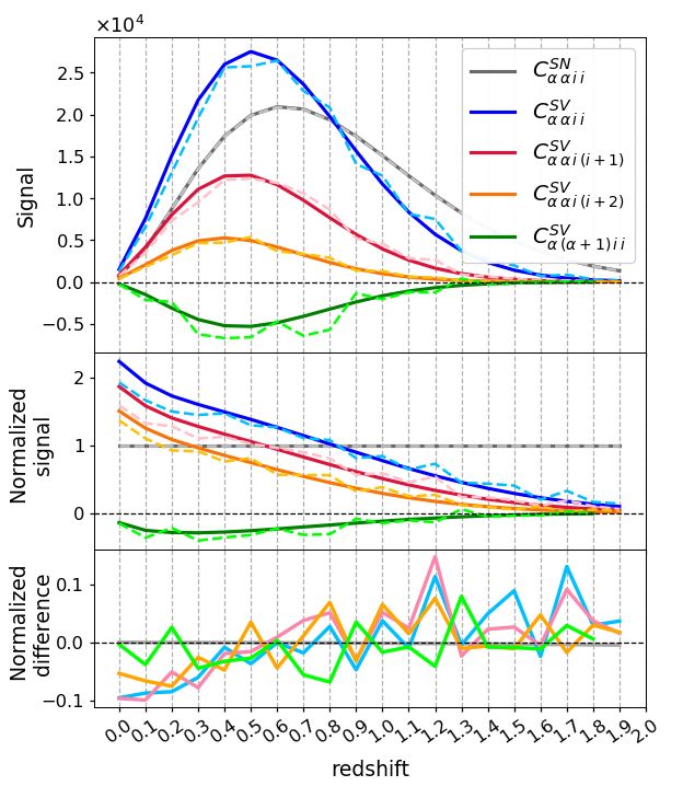
the various components, in Fig. 4 we show the covariance from 4.2. Redshift and mass binning
model and simulations for different terms and components of
the matrix, as a function of redshift: in blue we show the sample The optimal binning scheme should ensure to extract the maxi-
SV
variance diagonal terms (i.e. same mass and redshift bin, Cααii ), mum information from the data while avoiding wasting compu-
in red and orange the diagonal sample variance in two different tational resources with an exceedingly fine binning: adopting too
large bins would hide some information, while too small bins can
j with respectively j = i + 1 and j = i + 2),
SV
mass bins (Cααi
saturate the extractable information, making the analyses unnec-
in green the sample variance between two adjacent redshift bins
essarily computationally expensive. Moreover, too narrow bins
SV
(Cαβii , β = α + 1) and in gray the shot-noise variance (Cααii
SN
). In
could undermine the validity of the Gaussian approximation due
the upper panel we show the full covariance, in the central panel to the low occupancy numbers. This can happen also at high red-
the covariance normalized as in Eq. (24) and in the lower panel shift, where the number density of halos drops fast.
the normalized difference between model and simulations. Con- To establish the best binning scheme for the Poissonian like-
firming what was noticed from Fig. 3, the block-diagonal sample lihood function, we analyze the data assuming four redshift bin
variance terms are the dominant sources of error at low redshift, widths ∆z = {0.03, 0.1, 0.2, 0.3} and three numbers of mass bins
with a signal that rapidly decreases when considering different N M = {50, 200, 300}. In Fig. 5 we show the FoM as a func-
mass bins (blue, red and orange lines). Shot-noise dominates at tion of ∆z, for different mass binning. Since each result of the
high redshift and in the off-diagonal terms. We also observe that likelihood maximization process is affected by some statistical
the cross-correlation between different redshift bins produces a noise, the points represent the mean values obtained from 5 re-
small anti-correlation, whose relevance however seems negligi- alizations (which are sufficient for a consistent average result),
ble; further considerations about this point will be presented in with the corresponding standard error. About the redshift bin-
Sect. 4.3. ning, the curve increases with decreasing ∆z and flattens below
∆z ∼ 0.2; from this result we conclude that for bin widths . 0.2
the information is fully preserved and, among these values, we
choose ∆z = 0.1 as the bin width that maximize the informa-
Regarding the comparison between model and simulations, tion. The change of the mass binning affects the results in a mi-
the figure clearly shows that the analytical model reproduces nor way, giving points that are consistent with each other for all
with good agreement the covariance from simulations, with de- the redshift bin widths. To better study the effect of the mass
viations within the 10 per cent level. Part of such differences can binning, we compute the FoM also for N M = {5, 500, 600} at
be ascribed to the statistical noise, which produces random fluc- ∆z = 0.1, finding that the amount of recovered information satu-
tuations in the simulated covariance matrix. We also observe, rates around N M = 300. Thus, we use N M = 300 for the Poisso-
mainly on the block-diagonal terms, a slight underestimation of nian likelihood case, corresponding to ∆ log10 (M/M ) = 0.007.
the correlation at low redshift and a small overestimation at high We repeat the analysis for the Gaussian likelihood (with
redshift, which are consistent with the under/overestimation of full covariance), by considering the redshift bin widths ∆z =
the T10 halo bias shown in Fig. 2. Additional analyses are pre- {0.1, 0.2, 0.3} and three numbers of mass bins N M = {5, 7, 10},
sented in Appendix A, where we treat the description of the plus N M = {2, 20} for ∆z = 0.1. We do not include the case of
model with a spherical top-hat window function. Nevertheless, a tighter redshift or mass binning, to avoid deviating too much
this discrepancy on the covariance errors has negligible effects from the Gaussian limit of large occupancy numbers. The result
on the parameter constraints, at this level of statistics. This com- for the FoM is shown Fig. 6, from which we can state that also
parison will be further analyzed in Sect. 4.3. for the Gaussian case the curve starts to flatten around ∆z ∼ 0.2
Article number, page 7 of 15A&A proofs: manuscript no. PAPER
Fig. 5. Figure of merit for the Poissonian likelihood as a function of
the redshift bin widths, for different numbers of mass bins. The points
represent the average value over 5 realizations and the error bars are the
standard error of the mean. A small horizontal offset has been applied
to make the comparison clearer.
Fig. 4. Covariance (upper panel) and covariance normalized to the shot-
noise level (central panel) as predicted by the Hu & Kravtsov (2003)
analytical model (solid lines) and by simulations (dashed lines) for dif-
ferent matrix components: diagonal sample variance terms in blue, diag-
onal sample variance terms in two different mass bins in red and orange,
sample variance between two adjacent redshift bins in green and shot-
noise in gray. Lower panel: relative difference between analytical model
and simulations. The curves are represented as a function of redshift, in
the first mass bin (i = 1).
and ∆z = 0.1 results to be the optimal redshift binning, since
for larger bin widths less information is extracted and for tighter
bins the number of objects becomes too low for the validity of
the Gaussian limit. Also in this case the mass binning does not
influence the results in a significant way, provided that the num- Fig. 6. Same as Fig. 5, for the Gaussian likelihood.
ber of binning is not too low. We decide to use N M = 5, corre-
sponding to the mass bin widths ∆ log10 (M/M ) = 0.4.
ance. In contrast, the inclusion of the sample covariance (blue
4.3. Likelihood comparison and black contours) produces wider contours (and smaller FoM),
indicating that neglecting this effect leads to an underestimation
In this section we present the comparison between the posteriors of the error on the parameters. Also, there is no significant differ-
of cosmological parameters obtained by applying the different ence in using the covariance matrix from simulations or the an-
definitions of likelihood results on the entire sample of light- alytical model, since the difference in the FoM is below the per-
cones, by considering the average likelihood defined by Eq. (8). cent level. This result means that the level of accuracy reached
The first result is shown in Fig. 7, which represents the pos- by the model is sufficient to obtain an unbiased estimation of pa-
teriors derived from the three likelihood functions: Poissonian, rameters in a survey of galaxy clusters having sky coverage and
Gaussian with only shot-noise and Gaussian with shot-noise and cluster statistics comparable to that of the Euclid survey. Ac-
sample variance (Eqs. 5, 6 and 7, respectively). For the latter we cording to this conclusion, we will use the analytical covariance
compute the analytical covariance matrix at the input cosmology matrix to describe the statistical errors for all following likeli-
and compare it with the results obtained by using the covariance hood evaluations.
matrix from simulations. The corresponding FoM in the σ8 – Having established that the inclusion of the sample variance
Ωm plane is shown in Fig. 8. The first two cases look almost the has a non-negligible effect on parameter posteriors, we focus on
same, meaning that a finer mass binning as the one adopted in the Gaussian likelihood case. In Fig. 9 we show the results ob-
the Poisson likelihood does not improve the constraining power tained by using the full covariance matrix and only the block-
compared to the results from a Gaussian plus shot-noise covari- diagonal of such matrix (Ci jαα ), i.e. considering shot-noise and
Article number, page 8 of 15A. Fumagalli et al.: Euclid: Effect of sample covariance on the number counts of galaxy clusters
Fig. 7. Contour plots at 68 and 95 per cent of confidence level for Fig. 9. Contour plots at 68 and 95 per cent of confidence level for the
the three likelihood functions: Poissonian (red), Gaussian with only Gaussian likelihood with full covariance (blue) and the Gaussian like-
shot-noise (orange) and Gaussian with shot-noise and sample variance, lihood with block-diagonal covariance (black). The grey dotted lines
with covariance from the analytical model (blue) and from simulations represent the input values of parameters.
(black). The grey dotted lines represent the input values of parameters.
the correlation between redshift bins produces a minor effect on
the parameter posteriors. However, the difference between the
two FoMs is not necessarily negligible: for three parameters, a
∼25% change in the FoM corresponds to a potential underesti-
mate of the parameter errorbar by ∼10%. The Euclid Consortium
is presently requiring for the likelihood estimation that approx-
imations should introduce a bias in parameter errorbars that is
smaller than 10%, so as not to impact the first significant digit of
the error. Because the list of potential systematics at the required
precision level is long, one should avoid any oversimplification
that alone induces such a sizeable effect. The full covariance is
thus required to properly describe the sample variance effect at
the Euclid level of accuracy.
4.4. Cosmology dependence of covariance
We also investigate if there are differences in using a cosmology-
dependent covariance matrix instead of a cosmology-
independent one. In fact, the use of a matrix evaluated at
Fig. 8. Figure of merit for the different likelihood models: Poissonian, a fixed cosmology can represent an advantage, by reducing
Gaussian with shot-noise, Gaussian with full covariance from simula- the computational cost, but may bias the results. In Fig. 10 we
tions, Gaussian with full covariance from the model and Gaussian with compare the parameters estimated with a cosmology-dependent
block-diagonal covariance from the model. covariance (black contours), i.e. recomputing the covariance at
each step of the MCMC process, with the posteriors obtained by
evaluating the matrix at the input cosmology (blue), or assuming
sample variance effects between masses at the same redshift but a slightly lower/higher value for Ωm , log10 As and σ8 (red and
no correlation between different redshift bins. The resulting con- orange contours, respectively), chosen in order to have depar-
tours present small differences, as can be seen from the compar- tures from the fiducial values of the order of 2σ from Planck
ison of the FoM in Fig. 8: the difference in the FoM between the Collaboration et al. (2020). Specifically, we fix the parameter
diagonal and full covariance cases is about one third of the effect values at Ωm = 0.295, log10 As = −8.685 and σ8 = 0.776 for the
generated by the inclusion of the full covariance with respect the lower case and Ωm = 0.320, log10 As = −8.625 and σ8 = 0.884
only shot-noise cases. This means that, at this level of statistics for the higher case. We notice, also from the FoM comparison in
and for this redshift binning, the main contribution to the sample Fig. 11, that there is no appreciable difference between the first
covariance comes from the correlation between mass bins, while two cases. In contrast, when a wrong-cosmology covariance
Article number, page 9 of 15A&A proofs: manuscript no. PAPER
5. Discussion and conclusions
In this work we studied some of the theoretical systematics
that can affect the derivation of cosmological constraints from
the analysis of number counts of galaxy clusters from a survey
having sky-coverage and selection function similar to those ex-
pected for the photometric Euclid cluster survey. One of the aims
of the paper was to understand if the inclusion of sample vari-
ance, in addition to the shot-noise error, could have some influ-
ence on the estimation of cosmological parameters, at the level
of statistics that will be reached by the future Euclid catalogs.
Note that in this work we only consider uncertainties which do
not deal with observations, thus neglecting the systematics re-
lated to the mass estimation; however Köhlinger et al. (2015)
state that for Euclid the mass estimates from weak lensing will
be under control and, although there will be still additional sta-
tistical and systematic uncertainties due to mass calibration, the
analysis of real catalogs will approach the ideal case considered
here.
To describe the contribution of shot-noise and sample vari-
ance, we computed an analytical model for the covariance ma-
trix, representing the correlation between mass and redshift bins
as a function of cosmological parameters. Once the model for the
covariance has been properly validated, we moved to the iden-
Fig. 10. Contour plots at 68 and 95 per of cent confidence level for tification of the more appropriate likelihood function to analyse
the Gaussian likelihood evaluated with: a cosmology-dependent covari- cluster abundance data. The likelihood analysis has been per-
ance matrix (black), a covariance matrix fixed at the input cosmology formed with only two free parameters, Ωm and log10 As (and thus
(blue) and covariance matrices computed at two wrong cosmologies, σ8 ), since the mass function is less affected by the variation of
one with lower parameter values (Ωm = 0.295, log10 As = −8.685 and the other cosmological parameters.
σ8 = 0.776, red) and one with higher parameter values (Ωm = 0.320, Both the validation of the analytical model for the covari-
log10 As = −8.625 and σ8 = 0.884, orange). The grey dotted lines rep- ance matrix and the comparison between posteriors from dif-
resent the input values of parameters. ferent likelihood definitions are based on the analysis of an ex-
tended set of 1000 Euclid–like past-light cones generated with
the LPT-based PINOCCHIO code (Monaco et al. 2002; Munari
et al. 2017).
The main results of our analysis can be summarized as fol-
lows.
– To include the sample variance effect in the likelihood anal-
ysis, we computed the covariance matrix from a large set of
mock catalogs. Most of the sample variance signal is con-
tained in the block-diagonal terms of the matrix, giving a
contribution larger than the shot-noise term, at least in the
low-mass/low-redshift regime. On the other hand, the anti-
correlation between different redshift bins produces a minor
effect with respect to the diagonal variance.
– We computed the covariance matrix by applying the analyt-
ical model by Hu & Kravtsov (2003), assuming the appro-
priate window function, and verified that it reproduces the
matrix from simulations with deviations below the 10 per-
cent accuracy; this difference can be ascribed mainly to the
non-perfect match of the T10 halo bias with the one from
simulations. However, we verified that such a small differ-
ence does not affect the inference of cosmological parame-
ters in a significant way, at the level of statistic of the Euclid
Fig. 11. Figure of merit for the models described in Fig. 10. survey. Therefore we conclude that the analytical model of
Hu & Kravtsov (2003) can be reliably applied to compute a
cosmology-dependent, noise-free covariance matrix, without
requiring a large number of simulations.
matrix is used we can find either tighter or wider contours, – We established the optimal binning scheme to extract the
meaning that the effect of shot-noise and sample variance can be maximum information from the data, while limiting the com-
either under- or over-estimated. Thus, the use of a cosmology- putational cost of the likelihood estimation. We analyzed the
independent covariance matrix in the analysis of real cluster halo mass function with a Poissonian and a Gaussian like-
abundance data might lead to under/overestimated parameter lihood, for different redshift- and mass-bin widths and then
uncertainties at the level of statistic expected for Euclid. computed the figure of merit from the resulting contours in
Article number, page 10 of 15A. Fumagalli et al.: Euclid: Effect of sample covariance on the number counts of galaxy clusters
Ωm – σ8 plane. The results show that, both for the Poissonian Fundação para a Ciência e a Tecnologia, the Ministerio de Economia y Com-
and the Gaussian likelihood, the optimal redshift bin width is petitividad, the National Aeronautics and Space Administration, the Nether-
landse Onderzoekschool Voor Astronomie, the Norwegian Space Agency, the
∆z = 0.1: for larger bins, not all the information is extracted, Romanian Space Agency, the State Secretariat for Education, Research and In-
while for smaller bins the Poissonian case saturates and the novation (SERI) at the Swiss Space Office (SSO), and the United Kingdom
Gaussian case is no longer a valid approximation. The mass Space Agency. A complete and detailed list is available on the Euclid web site
binning affects less the results, provided not to choose a too (http://www.euclid-ec.org).
small number of bins. We decided to use N M = 300 for the
Poissonian likelihood and N M = 5 for the Gaussian case.
– We included the covariance matrix in the likelihood analy- References
sis and demonstrated that the contribution to the total error
budget and the correlation induced by the sample variance Albrecht, A., Bernstein, G., Cahn, R., et al. 2006, arXiv e-prints, arXiv:0609591
Allen, S. W., Evrard, A. E., & Mantz, A. B. 2011, ARA&A, 49, 409
term cannot be neglected. In fact, the Poissonian and Gaus- Anderson, T. 2003, An Introduction to Multivariate Statistical Analysis, Wiley
sian with shot-noise likelihood functions show smaller er- Series in Probability and Statistics (Wiley)
rorbars with respect to the Gaussian with covariance likeli- Artis, E., Melin, J.-B., Bartlett, J. G., & Murray, C. 2021 [arXiv:2101.02501]
hood, meaning that neglecting the sample covariance leads Bertocco, S., Goz, D., Tornatore, L., et al. 2019, arXiv e-prints,
arXiv:1912.05340
to an underestimation of the error on parameters, at the Eu- Bocquet, S., Dietrich, J. P., Schrabback, T., et al. 2019, ApJ, 878, 55
clid level of accuracy. As shown in Appendix B, this result Bocquet, S., Heitmann, K., Habib, S., et al. 2020, ApJ, 901, 5
holds also for the eROSITA survey, while it is not valid for Bocquet, S., Saro, A., Dolag, K., & Mohr, J. J. 2016, MNRAS, 456, 2361
present surveys like Planck and SPT. Bocquet, S., Saro, A., Mohr, J. J., et al. 2015, ApJ, 799, 214
Bond, J. R. & Myers, S. T. 1996, ApJS, 103, 1
– We verified that the anti-correlation between bins at different Borgani, S., Plionis, M., & Kolokotronis, E. 1999, MNRAS, 305, 866
redshifts produces a minor, but non-negligible effect on the Bouchet, F. R., Colombi, S., Hivon, E., & Juszkiewicz, R. 1995, A&A, 296, 575
posteriors of cosmological parameters at the level of statis- Buchert, T. 1992, MNRAS, 254, 729
Buchner, J., Georgakakis, A., Nandra, K., et al. 2014, A&A, 564, A125
tics reached by the Euclid survey. We also established that Carlstrom, J. E., Ade, P. A. R., Aird, K. A., et al. 2011, PASP, 123, 568
a cosmology-dependent covariance matrix is more appropri- Castro, T., Borgani, S., Dolag, K., et al. 2021, MNRAS, 500, 2316
ate than the cosmology-independent case, which can lead to Cataneo, M. & Rapetti, D. 2018, Int. J. Mod. Phys. D, 27, 1848006
biased results due to the wrong quantification of shot-noise Costanzi, M., Rozo, E., Simet, M., et al. 2019, MNRAS, 488, 4779
Costanzi, M., Sartoris, B., Xia, J.-Q., et al. 2013, J. Cosmology Astropart. Phys.,
and sample variance. 2013, 020
Cui, W., Borgani, S., & Murante, G. 2014, MNRAS, 441, 1769
One of the main results of the analysis presented here is that, DES Collaboration, Abbott, T., Aguena, M., et al. 2020, arXiv e-prints,
for next generation surveys of galaxy clusters, such as Euclid, arXiv:2002.11124
Despali, G., Giocoli, C., Angulo, R. E., et al. 2016, MNRAS, 456, 2486
sample variance effects need to be properly included, becoming Diemer, B. 2017, ApJS, 231, 5
one of the main sources of statistical uncertainty in the cosmo- Diemer, B. 2020, arXiv e-prints, arXiv:2007.10346
logical parameters estimation process. The correct description of Eisenstein, D. J. & Loeb, A. 1995, ApJ, 439, 520
sample variance is guaranteed by the analytical model validated Euclid Collaboration: Adam, R., Vannier, M., Maurogordato, S., et al. 2019,
A&A, 627, A23
in this work. Hartlap, J., Simon, P., & Schneider, P. 2007, A&A, 464, 399
This analysis represents the first step towards providing all Heavens, A. 2009, arXiv e-prints, arXiv:0906.0664
the necessary ingredients for an unbiased estimation of cos- Heitmann, K., Bingham, D., Lawrence, E., et al. 2016, ApJ, 820, 108
mological parameters from the number counts of galaxy clus- Hu, W. & Kravtsov, A. V. 2003, ApJ, 584, 702
Jenkins, A., Frenk, C. S., White, S., et al. 2001, MNRAS, 321, 372
ters. It has to be complemented with the characterization of the Köhlinger, F., Hoekstra, H., & Eriksen, M. 2015, MNRAS, 453, 3107
other theoretical systematics, e.g. related to the calibration of the Kravtsov, A. V. & Borgani, S. 2012, ARA&A, 50, 353
halo mass function, and observational systematics, related to the Lacasa, F., Lima, M., & Aguena, M. 2018, Astron. Astrophys., 611, A83
mass-observable relation and to the cluster selection function. Lacasa, F. & Rosenfeld, R. 2016, J. Cosmology Astropart. Phys., 08, 005
Laureijs, R., Amiaux, J., Arduini, S., et al. 2011, arXiv e-prints, arXiv:1110.3193
To further improve the extractable information from galaxy Mana, A., Giannantonio, T., Weller, J., et al. 2013, MNRAS, 434, 684
clusters, the same analysis will be extended to the clustering of Manera, M. & Gaztañaga, E. 2011, MNRAS, 415, 383
galaxy clusters, by analyzing the covariance of the power spec- Mantz, A. B., von der Linden, A., Allen, S. W., et al. 2015, MNRAS, 446, 2205
McClintock, T., Rozo, E., Becker, M. R., et al. 2019, ApJ, 872, 53
trum or of the two-point correlation function. Once all the sys- Monaco, P. 2016, Galaxies, 4, 53
tematics will be calibrated, so as to properly combine such two Monaco, P., Theuns, T., & Taffoni, G. 2002, MNRAS, 331, 587
observables (Schuecker et al. 2003; Mana et al. 2013; Lacasa & Moutarde, F., Alimi, J. M., Bouchet, F. R., Pellat, R., & Ramani, A. 1991, ApJ,
Rosenfeld 2016), number counts and clustering of galaxy clus- 382, 377
Munari, E., Monaco, P., Sefusatti, E., et al. 2017, MNRAS, 465, 4658
ters will provide valuable observational constraints, complemen- Nakamura, T. T. & Suto, Y. 1997, Progress of Theoretical Physics, 97, 49
tary to those of the other two main Euclid probes, namely galaxy Planck Collaboration, Ade, P. A. R., Aghanim, N., et al. 2014, A&A, 571, A16
clustering and cosmic shear. Planck Collaboration, Aghanim, N., Akrami, Y., et al. 2020, A&A, 641, A6
Pratt, G. W., Arnaud, M., Biviano, A., et al. 2019, Space Sci. Rev., 215, 25
Acknowledgements. We would like to thank Laura Salvati for useful discus- Predehl, P. 2014, Astronomische Nachrichten, 335, 517
sions about the selection functions. SB, AS and AF acknowledge financial sup- Press, W. & Schechter, P. 1974, ApJ, 187, 425
port from the ERC-StG ’ClustersxCosmo’ grant agreement 716762, the PRIN- Sahni, V. & Coles, P. 1995, Phys. Rep., 262, 1
MIUR 2015W7KAWC grant, the ASI-Euclid contract and the INDARK grant. Salvati, L., Douspis, M., & Aghanim, N. 2020, A&A, 643, A20
TC is supported by the INFN INDARK PD51 grant and by the PRIN-MIUR Sartoris, B., Biviano, A., Fedeli, C., et al. 2016, MNRAS, 459, 1764
2015W7KAWC grant. Our analyses have been carried out at: CINECA, with the Sartoris, B., Borgani, S., Fedeli, C., et al. 2010, MNRAS, 407, 2339
projects INA17_C5B32 and IsC82_CosmGC; the computing center of INAF- Sartoris, B., Borgani, S., Rosati, P., & Weller, J. 2012, MNRAS, 423, 2503
Osservatorio Astronomico di Trieste, under the coordination of the CHIPP Schuecker, P., Böhringer, H., Collins, C. A., & Guzzo, L. 2003, A&A, 398, 867
project (Bertocco et al. 2019; Taffoni et al. 2020). The Euclid Consortium ac- Sheth, R. K. & Tormen, G. 2002, MNRAS, 329, 61
knowledges the European Space Agency and a number of agencies and institutes Taffoni, G., Becciani, U., Garilli, B., et al. 2020, arXiv e-prints,
that have supported the development of Euclid, in particular the Academy of arXiv:2002.01283
Finland, the Agenzia Spaziale Italiana, the Belgian Science Policy, the Cana- Tauber, J. A., Mandolesi, N., Puget, J. L., et al. 2010, A&A, 520, A1
dian Euclid Consortium, the Centre National d’Etudes Spatiales, the Deutsches Taylor, A., Joachimi, B., & Kitching, T. 2013, MNRAS, 432, 1928
Zentrum für Luft- und Raumfahrt, the Danish Space Research Institute, the Tinker, J., Kravtsov, A. V., Klypin, A., et al. 2008, ApJ, 688, 709
Article number, page 11 of 15You can also read