An SPH framework for fluid-solid and contact interaction problems including thermo-mechanical coupling and reversible phase transitions
←
→
Page content transcription
If your browser does not render page correctly, please read the page content below
Fuchs et al. Adv. Model. and Simul.
in Eng. Sci.(2021)8:15
https://doi.org/10.1186/s40323-021-00200-w

    RESEARCH ARTICLE                                                                                                                          Open Access

An SPH framework for fluid–solid and
contact interaction problems including
thermo-mechanical coupling and
reversible phase transitions
Sebastian L. Fuchs1,2 , Christoph Meier1 , Wolfgang A. Wall1                                       and Christian J. Cyron2,3*

* Correspondence:

christian.cyron@hereon.de               Abstract
3
 Institute of Material Systems
Modeling, Helmholtz-Zentrum
                                        The present work proposes an approach for fluid–solid and contact interaction
Hereon, Max-Planck-Straße 1,            problems including thermo-mechanical coupling and reversible phase transitions. The
21502 Geesthacht, Germany               solid field is assumed to consist of several arbitrarily-shaped, undeformable but mobile
Full list of author information is
available at the end of the article
                                        rigid bodies, that are evolved in time individually and allowed to get into mechanical
                                        contact with each other. The fluid field generally consists of multiple liquid or gas
                                        phases. All fields are spatially discretized using the method of smoothed particle
                                        hydrodynamics (SPH). This approach is especially suitable in the context of continually
                                        changing interface topologies and dynamic phase transitions without the need for
                                        additional methodological and computational effort for interface tracking as compared
                                        to mesh- or grid-based methods. Proposing a concept for the parallelization of the
                                        computational framework, in particular concerning a computationally efficient
                                        evaluation of rigid body motion, is an essential part of this work. Finally, the accuracy
                                        and robustness of the proposed framework is demonstrated by several numerical
                                        examples in two and three dimensions, involving multiple rigid bodies, two-phase flow,
                                        and reversible phase transitions, with a focus on two potential application scenarios in
                                        the fields of engineering and biomechanics: powder bed fusion additive manufacturing
                                        (PBFAM) and disintegration of food boluses in the human stomach. The efficiency of
                                        the parallel computational framework is demonstrated by a strong scaling analysis.
                                        Keywords: Rigid body motion, Two-phase flow, Reversible phase transitions,
                                        Smoothed particle hydrodynamics, Metal additive manufacturing, Gastric fluid
                                        mechanics

                                      Introduction
                                      In many applications in science and engineering, like for example in some areas of biome-
                                      chanics, fluid–solid and contact interaction problems characterized by a large number
                                      of solid bodies immersed in a fluid flow and undergoing reversible phase transitions,
                                      are of great interest. Often, explicitly considering the deformation of solid bodies can
                                      be neglected, which reduces the complexity of the problem to the treatment of unde-

                                      © The Author(s) 2021, corrected publication 2021. This article is licensed under a Creative Commons Attribution 4.0 International
                                      License, which permits use, sharing, adaptation, distribution and reproduction in any medium or format, as long as you give
                                      appropriate credit to the original author(s) and the source, provide a link to the Creative Commons licence, and indicate if changes
                                      were made. The images or other third party material in this article are included in the article’s Creative Commons licence, unless
                                      indicated otherwise in a credit line to the material. If material is not included in the article’s Creative Commons licence and your
                                      intended use is not permitted by statutory regulation or exceeds the permitted use, you will need to obtain permission directly
                                      from the copyright holder. To view a copy of this licence, visit http://creativecommons.org/licenses/by/4.0/.

                                                                                                                                                   0123456789().,–: volV
Fuchs et al. Adv. Model. and Simul. in Eng. Sci.(2021)8:15                                                          Page 2 of 33

                   formable but mobile rigid bodies, in favor of simplified modeling. Most current mesh- or
                   grid-based methods, e.g., the finite element method (FEM), the finite difference method
                   (FDM), or the finite volume method (FVM), require substantial methodological and com-
                   putational efforts to model the motion of rigid bodies in fluid flow. To overcome those
                   issues, several approaches, e.g., based on the particle finite element method (PFEM) [1–3],
                   on the discrete element method (DEM) [4–7], or on smoothed particle hydrodynamics
                   (SPH) [8–14], have been proposed. SPH as a mesh-free discretization scheme is, due to its
                   Lagrangian nature, very well suited for flow problems involving multiple phases, dynamic
                   and reversible phase transitions, and complex interface topologies. This makes SPH very
                   appropriate for a wide range of applications in engineering, e.g., in metal additive manu-
                   facturing melt pool modeling [15,16], or in biomechanics, e.g., for modeling the digestion
                   of food in the human stomach [17]. For the former application, an SPH formulation for
                   thermo-capillary phase transition problems involving solid, liquid, and gaseous phases
                   has recently been proposed [18], amongst others, focusing on evaporation-induced recoil
                   pressure forces, temperature-dependent surface tension and wetting forces, Gaussian laser
                   beam heat sources, and evaporation-induced heat losses. However, for simplicity, this and
                   also other current state-of-the-art approaches, e.g., [19,20] are restricted to immobile
                   powder grains.
                     All aforementioned SPH formulations for modeling rigid body motion in fluid flow have
                   in common, that rigid bodies are fully resolved, that is spatially discretized as clusters of
                   particles. It is generally accepted that advanced boundary particle methods, e.g., based
                   on the extrapolation of field quantities from fluid to boundary particles [21–23], are
                   beneficial, because one can model the fluid field close to the boundary with high accuracy.
                   In many of the aforementioned applications, an exact representation of the fluid–solid
                   interface plays an important role. Therefore, herein a formulation of this kind proposed
                   in [23] is utilized. To the best of the authors’ knowledge none of the aforementioned SPH
                   formulations modeling rigid body motion in fluid flow simultaneously consider thermal
                   conduction, reversible phase transitions, and multiple (liquid and gas) phases.
                     To help close this gap, this contribution proposes a fully resolved smoothed particle
                   hydrodynamics framework for fluid–solid and contact interaction problems including
                   thermo-mechanical coupling and reversible phase transitions. The solid field is assumed
                   to consist of several arbitrarily-shaped, undeformable but mobile rigid bodies, that are
                   evolved in time individually. Based on a temperature field, provided by solving the
                   heat equation, reversible phase transitions, i.e., melting and solidification, are evaluated
                   between the fluid and the solid field. As a result, the shape and the total number of rigid
                   bodies may vary over time. In addition, contact between rigid bodies is considered by
                   employing a spring-dashpot model. Note that some characteristic phenomena for thermo-
                   capillary flow [24,25] and, especially, for metal PBFAM melt pool modeling [18–20,26–28]
                   are not addressed in this work, thus, referring to the literature.
                     While parallel implementation aspects along with detailed scalability studies are not in
                   the focus of the aforementioned references, in this work, a concept for the parallelization
                   of the computational framework is proposed, setting the focus in particular on an efficient
                   evaluation of rigid body motion. The parallel behavior is demonstrated, confirming that
                   detailed studies at a large scale become possible. It shall be noted, that the parallel imple-
                   mentation of such a computational framework is far from trivial but indispensable when
                   examining numerical examples that are of practical relevance. Note that the introduced
Fuchs et al. Adv. Model. and Simul. in Eng. Sci.(2021)8:15                                                                                  Page 3 of 33

                     Fig. 1 Domain  consisting of several disjunct domains, the fluid domain f and the solid sub-domains sk
                     representing rigid bodies k, with fluid–solid interface kfs and solid-solid interface  ss in the event of contact
                                                                                                            k,k̂
                     between the rigid bodies k and k̂

                   concept for the parallelization of the computational framework is applicable not only
                   when using SPH as a discretization scheme, but also for other particle-based methods,
                   e.g., discrete element method (DEM), or molecular dynamics (MD).
                     The remainder of this work is organized as follows: To begin with, the governing equa-
                   tions for a fluid–solid and contact interaction problem including thermo-mechanical
                   coupling and reversible phase transition are outlined. Next, the numerical methods are
                   presented and the details of the computational framework are discussed. Finally, the accu-
                   racy and robustness of the proposed formulation is demonstrated by several numerical
                   examples.

                   Governing equations
                   Consider a domain  of a fluid–solid interaction problem that consists at each time t ∈
                   [0, T ] of the non-overlapping fluid domain f and solid domain s that share a common
                   interface  fs , with  = f ∪ s and f ∩ s =  fs . In general, the fluid domain f
                   may consist of multiple (liquid and gas) phases. For ease of notation, in the following
                   it will not be distinguished between the different fluid phases. The solid domain s is
                   composed of several non-overlapping sub-domains sk , which represent rigid bodies k,

                   such that s = k sk . In the event of contact between two rigid bodies k and k̂, a
                   common interface  ss = sk ∩ s exists, separating the two solid sub-domains sk and
                                          k,k̂           k̂
                   s . A detailed illustration of the problem is given in Fig. 1. In the following the (standard)
                      k̂
                   governing equations of the fluid and the solid field as well as the respective coupling
                   conditions are briefly given. In addition, reversible phase transitions between the fluid
                   and the solid field, e.g., temperature-induced melting and solidification, may occur. For
                   this reason, the temperature field is modeled solving the heat equation.

                   Fluid field
                   The fluid field is governed by the instationary Navier–Stokes equations in the domain f ,
                   which consist in convective form of the mass continuity equation and the momentum
                   equation

                          dρ f
                               = −ρ f ∇ · uf in f ,                                                                                  (1)
                           dt
                          duf      1
                               = − f ∇ pf + fν + bf in f ,                                                                           (2)
                           dt     ρ
Fuchs et al. Adv. Model. and Simul. in Eng. Sci.(2021)8:15                                                            Page 4 of 33

                   with viscous force fν and body force bf each per unit mass. For a Newtonian fluid the
                   viscous force is fν = ν f ∇ 2 uf with kinematic viscosity ν f . The mass continuity equation (1)
                   and the momentum equation (2) represent a system of d + 1 equations with the d + 2
                   unknowns, velocity uf , density ρ f , and pressure pf , in d-dimensional space. The system
                   of equations is closed with an equation of state pf = pf (ρ f ) relating fluid density ρ f and
                   pressure pf . The Navier–Stokes equations (1) and (2) are subject to the following initial
                   conditions

                                     f                            f
                         ρ f = ρ0         and uf = u0 in f                      at t = 0                      (3)

                                               f                                 f
                   with initial density ρ0 and initial velocity u0 . In addition, Dirichlet and Neumann boundary
                   conditions are applied on the fluid boundary  f = ∂f \  fs

                                                   f                                     f
                         uf = ûf         on D and t f = t̂ f                   on N ,                       (4)

                                                                                                          f      f
                   with prescribed boundary velocity ûf and boundary traction t̂ f , where  f = D ∪ N
                         f     f                                                         fs
                   and D ∩ N = ∅. Furthermore, on the fluid–solid interface  fs = k k the so-called
                   kinematic and dynamic coupling conditions are

                                     fs                          fs        fs
                         u f = uk         and t f = tk                on k      ∀k ,                          (5)

                   resembling a no-slip boundary condition and ensuring equilibrium of fluid and solid
                                                                 fs     fs
                   traction across the interface  fs . Herein, uk and tk denote the velocity respectively traction
                                                                                        fs
                   of a rigid body k on the fluid–solid interface k .

                   Remark 1 In Eqs. (1)–(2) governing the fluid field, all time derivatives follow the motion
                                                                           ∂(·)
                   of material points, i.e., are material derivatives d(·)
                                                                      dt = ∂t + u · ∇(·). Besides, ∇(·) denotes
                   derivatives with respect to spatial coordinates.

                   Solid field
                   The solid field is assumed to consist of several mobile rigid bodies k each represented by
                   a sub-domain sk embedded in the fluid domain f . Thus, the interface of a rigid body k

                             fs
                   is ks = k ∪        ss
                                     k̂ k,k̂ with contacting rigid bodies k̂, cf. Fig. 1. The kinematics of each
                   rigid body k are uniquely defined by three respectively six degrees of freedom in two- and
                   three-dimensional space, i.e., the position of the center of mass rks and the orientation ψsk .
                   As a result, the equations of motion of an individual rigid body k are described by the
                   balance of linear and angular momentum
                                 d2 rks     fs

                         msk            = f k  +   f ss + msk bsk               in sk ,                       (6)
                                 dt 2               k,k̂
                                                       k̂
                               dωsk    fs

                           Iks      = mk +   mss                       in sk ,                                (7)
                                dt            k,k̂
                                                            k̂

                   with mass msk and mass moment of inertia Iks with respect to the center of mass position rks .
                                                                                                                 fs
                   Herein, ωsk denotes the angular velocity of a rigid body k, cf. Remark 2. Furthermore, fk
                            fs
                   and mk describe the resultant coupling force respectively torque acting on the fluid–
                                          fs
                   solid interface k of rigid body k. Contacting rigid bodies k and k̂ exchange the resultant
Fuchs et al. Adv. Model. and Simul. in Eng. Sci.(2021)8:15                                                            Page 5 of 33

                   contact force f ss respectively torque mss at the solid-solid interface  ss . Finally, the body
                                  k,k̂                     k,k̂                             k,k̂
                   force bsk given per unit mass is contributing to the balance of linear momentum.

                   Remark 2 The orientation ψsk is expressed by a (pseudo-)vector whose direction and
                   magnitude represent the axis and angle of rotation. Note that in general, the angular
                   velocity ωsk of a rigid body k is different from the time derivative of the orientation ψsk ,
                   i.e., ωsk  = dψ sk /dt, due to the non-additivity of large rotations [29–32]. Direct evolution
                   of the orientation ψsk of a rigid body k requires a special class of time integration schemes,
                   so-called Lie group time integrators [33,34].

                   Thermal conduction
                   Thermal conduction in the combined fluid and solid domain  = f ∪ s in the absence
                   of heat sources or heat sinks (which are neglected herein for simplicity) is governed by
                   the heat equation

                               dT   1
                         cpφ      = φ ∇(κ φ ∇T ) in  ,                                                        (8)
                               dt  ρ

                                                                                                                 φ
                   with temperature T and heat flux q = −κ φ ∇T . The material parameters heat capacity cp
                   and thermal conductivity κ φ are in general different for fluid and solid field, and hence
                   for clarity are denoted by the index (·)φ with φ ∈ {f, s}. The heat equation (8) is subject to
                   the following initial condition

                         T = T0 in  at t = 0                                                                  (9)

                   with initial temperature T0 . In addition, Dirichlet and Neumann boundary conditions are
                   required on the domain boundary  = ∂

                         T = T̂      on D and q = q̂ on N ,                                                 (10)

                   with prescribed boundary temperature T̂ and boundary heat flux q̂, where  = D ∪ N
                   and D ∩ N = ∅.

                   Reversible phase transition
                   Reversible phase transitions, i.e., melting and solidification, are considered between the
                   solid and the fluid field. Within this publication, solid material points that exceed a transi-
                   tion temperature Tt undergo a phase transition to a fluid material point and vice versa, cf.
                   Remark 3. Consequently, the shape of a rigid body k, i.e., its sub-domain sk , is changing
                   due to a loss or gain of material points resulting in a varying mass mk , center of mass
                   position rk , and mass moment of inertia Ik .

                   Remark 3 For the sake of simplicity, only temperature-independent parameters are con-
                   sidered herein, and latent heat is neglected. Latent heat could be included by an apparent
                   capacity scheme relying on an increased heat capacity cp within a finite temperature
                   interval [35] in a straightforward manner.

                   Remark 4 The proposed framework is general enough to model also chemically-induced
                   phase transitions based on a concentration field. For this purpose, the diffusion equation
Fuchs et al. Adv. Model. and Simul. in Eng. Sci.(2021)8:15                                                                Page 6 of 33

                   dC/dt = 1/ρ φ ∇(Dφ ∇C) with diffusivity Dφ modeling the transport of a concentration C
                   is solved. Considering the similarity between the heat equation (8) and the diffusion equa-
                   tion, the latter can be discretized following a similar SPH discretization [36,37] as applied
                   for the heat equation. Similarly, modeling phase transitions a transition concentration Ct
                   is defined.

                   Numerical methods and parallel computational framework
                   This section presents the methods applied for discretization and numerical solution of
                   fluid–solid and contact interaction problems including thermo-mechanical coupling and
                   reversible phase transitions. The presented parallel computational framework is imple-
                   mented in the in-house parallel multiphysics research code BACI (Bavarian Advanced
                   Computational Initiative) [38] using the Message Passing Interface (MPI) for distributed-
                   memory parallel programming.

                   Spatial discretization via smoothed particle hydrodynamics
                   For the spatial discretization smoothed particle hydrodynamics (SPH) is used, allowing
                   for a straightforward particle-based evaluation of fluid–solid coupling conditions. In the
                   following, the basics of this method are recapitulated briefly.

                   Approximation of field quantities applying a smoothing kernel
                   The fundamental concept of SPH is based on the approximation of a field quantity f via a
                   smoothing operation and on the discretization of the domain  with discretization points,
                   so-called particles j, each occupying a volume Vj . Introducing a smoothing kernel W (r, h)
                   that fulfills certain consistency properties [36,39], cf. Remark 5, leads to an approximation
                   of the field quantity f based on summation of contributions from all particles j in the
                   domain

                         f (r) ≈           f (r )W (|r − r |, h)dr ≈        Vj f (rj )W (|r − rj |, h)            (11)
                                                                      j

                   which includes a smoothing error and a discretization error [40].

                   Remark 5 The smoothing kernel W (r, h) is a monotonically decreasing, smooth function
                   that depends on a distance r and a smoothing length h. The smoothing length h together
                   with a scaling factor κ define the support radius rc = κh of the smoothing kernel. Com-
                   pact support, i.e., W (r, h) = 0 for r > rc , as well as positivity, i.e., W (r, h) ≥ 0 for r ≤ rc ,
                   are typical properties of standard smoothing kernels W (r, h). In addition, the normaliza-

                   tion property requires that  W (|r − r |, h)dr = 1. The Dirac delta function property
                   limh→0 W (r, h) = δ(r) ensures an exact representation of a field quantity f in the limit
                   h → 0.

                     A straightforward approach in SPH to determine the gradient of a quantity f follows
                   directly by differentiation of (11) resulting in


                         ∇f (r) ≈            f (r )∇W (|r − rj |, h) dr ≈         Vj f (rj )∇W (|r − rj |, h) .   (12)
                                                                             j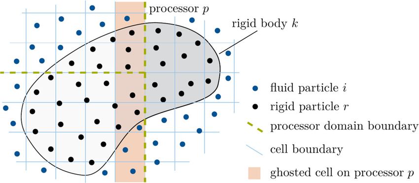
Fuchs et al. Adv. Model. and Simul. in Eng. Sci.(2021)8:15                                                            Page 7 of 33

                   Note that this (simple) gradient approximation shows some particular disadvantages.
                   Hence, more advanced approximations for gradients are given in the literature [36] and
                   will also be applied in the following. In sum, the concept of SPH allows to reduce partial
                   differential equations to a system of coupled ordinary differential equations (with as many
                   equations as particles) that is solved in the domain . Thereby, all field quantities are
                   evaluated at and associated with particle positions, meaning each particle carries its cor-
                   responding field quantities. Finally, in a post-processing step a continuous field quantity
                   f is recovered from the discrete quantities f (rj ) of particles j in the domain  using the
                   approximation (11) and the commonly known Shepard filter

                                      j Vj f (rj )W (|r − rj |, h)
                         fˆ (r) ≈                                 .                                          (13)
                                         j Vj W (|r − rj |, h)

                   Note that the denominator typically takes on values close to one inside the fluid domain
                   and is mainly relevant for boundary regions with reduced support due to a lack of neigh-
                   boring particles.

                   Remark 6 In the following, a quantity f evaluated for particle i at position ri is writ-
                   ten as fi = f (ri ). The short notation Wij = W (rij , h) denotes the smoothing kernel W
                   evaluated for particle i at position ri with neighboring particle j at position rj , where
                   rij = |rij | = |ri − rj | is the absolute distance between particles i and j. The deriva-
                   tive of the smoothing kernel W with respect to the absolute distance rij is denoted by
                   ∂W /∂rij = ∂W (rij , h)/∂rij .

                   Remark 7 Herein, a quintic spline smoothing kernel W (r, h) as defined in [21] with
                   smoothing length h and compact support of the smoothing kernel with support radius rc =
                   κh and scaling factor κ = 3 is used.

                   Initial particle spacing
                   Within this contribution, the domain  is initially filled with particles located on a regular
                   grid with particle spacing x, thus in the d-dimensional space each particle initially
                   occupies an effective volume Veff = ( x)d . A particle in the fluid domain f is called
                   a fluid particle i, whereas a particle in the solid domain sk of a rigid body k is called a
                   rigid particle r. It follows, that each rigid body is fully resolved being spatially discretized
                   as clusters of particles. Naturally, the choice of the particle spacing x influences the
                   accuracy of the interface representation between fluid and solid domain. The mass of a
                                                                                                               f
                   particle is initially assigned using the reference density of the respective phase, i.e., ρ0 for
                   the fluid phase and ρ0 for the solid phase, and the effective volume Veff .
                                            s

                   Remark 8 Within this work, the smoothing length h of the smoothing kernel W (r, h), cf.
                   Remark 7, is set equal to the initial particle spacing x. Consequently, in a convergence
                   analysis with decreasing particle spacing x the ratio x/h remains constant [40].

                   Parallelization via spatial decomposition of the domain
                   For the problems studied herein, an efficient parallel computational framework capable
                   of handling systems constituted of a large number of particles is required. This requires
                   addressing in particular two aspects, namely, an efficient particle neighbor pair detection,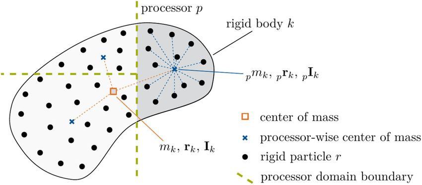
Fuchs et al. Adv. Model. and Simul. in Eng. Sci.(2021)8:15                                                                      Page 8 of 33

                     Fig. 2 A fluid–solid interaction problem consisting of a rigid body k with affiliated rigid particles r and
                     surrounding fluid particles i distributed over several processors p according to a spatial decomposition
                     approach

                   and a parallel load distribution strategy while keeping the communication overhead at an
                   acceptable level. In the literature, several approaches for parallel computational frame-
                   works utilizing particle-based methods have been proposed, e.g., [41–47]. In the present
                   work, a spatial decomposition approach with neighbor pair detection utilizing a combi-
                   nation of cell-linked lists and Verlet-lists based on [42] is applied. The general idea of the
                   spatial decomposition approach is briefly explained in the following, however, for detailed
                   information, the interested reader is referred to the original publication [42]. In addition,
                   the concept is extended herein to consider the motion of rigid bodies spatially discretized
                   as clusters of particles.
                      The evaluation of particle interactions in SPH requires knowledge of neighboring par-
                   ticles within a geometrically limited interaction distance, i.e., within the support radius rc
                   of the smoothing kernel. Thus, the computational domain is divided into several cubic
                   cells forming a uniform lattice, while each particle is uniquely assigned to one of those
                   cells according to its current spatial position, cf. Fig. 2. The size of the cells is chosen such
                   that neighboring particles are either located in the same cell or in adjacent cells, i.e., the
                   size of the cells is at least equal to the support radius rc of the smoothing kernel.
                      Following a spatial decomposition approach, the cells together with assigned particles
                   are distributed over all involved processors, i.e., forming so-called processor domains.
                   To keep the computational load balanced between all processors and to minimize the
                   communication overhead, cubic processor domains are defined such that each contains
                   (nearly) the same number of particles. The cells occupied by each processor are called
                   owned cells. On each processor the position of particles located in its processor domain,
                   i.e., the position of so-called owned particles, is evolved. This requires the evaluation of
                   interactions of owned particles with their neighboring particles. However, the correct
                   evaluation of particle interactions close to processor domain boundaries requires that
                   each processor has information not only about its owned particles but also about particles
                   in cells adjacent to its processor domain. To this end, each processor is provided full
                   information not only about its own domain but additionally about a layer of ghosted cells
                   (with ghosted particles) around its own domain. Keeping the information about ghosted
                   cells and particles continuously updated requires communication between processors.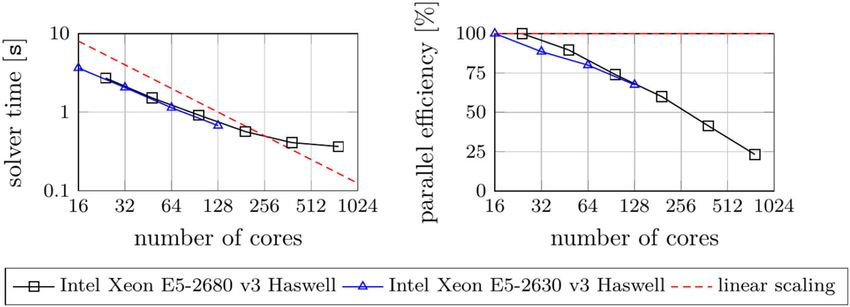
Fuchs et al. Adv. Model. and Simul. in Eng. Sci.(2021)8:15                                                            Page 9 of 33

                   Remark 9 To exemplify the cost of communication overhead, consider a perfectly cubic
                   processor domain occupying no owned cells. Consequently, assuming one layer of ghosted
                                                                            √
                   cells surrounding the processor domain, a total of ng = ( 3 no + 2)3 − no cells are ghosted.
                   That is, the communication overhead scales with the ratio ng /no of ghosted cells ng to
                   owned cells no . Furthermore, the (average) number of particles per cell, and, consequently,
                   also the communication overhead, scale with the ratio rc / x of the support radius rc and
                   the initial particle spacing x.

                     As a consequence of the spatial decomposition approach, the affiliated rigid particles r
                   of a rigid body k might be distributed over several processors, cf. Fig. 2. However, note that
                   the balance of linear and angular momentum, cf. Eqs. (6)–(7), describing the motion of a
                   rigid body k are given with respect to the center of mass position rks . Thus, the evaluation of
                   mass quantities, i.e., mass mk , center of mass position rks , and mass moment of inertia Ik ,
                   as well as the evaluation of resultant force fk and torque mk acting on a rigid body k,
                   requires special communication between all processors hosting rigid particles r belonging
                   to rigid body k and the single processor owning rigid body k.

                   Modeling fluid flow using weakly compressible SPH
                   For modeling fluid flow using SPH, several different formulations each with its own char-
                   acteristics and benefits can be derived. Here, the instationary Navier–Stokes equations (1)
                   and (2) are discretized by a weakly compressible approach [36,39,48]. This section gives
                   a brief overview of this formulation applied already in [18,49]. For ease of notation, in the
                   following the index (·)f denoting fluid quantities is dropped.

                   Density summation
                   The density of a particle i is determined via summation of the respective smoothing kernel
                   contributions of all neighboring particles j within the support radius rc

                         ρi = mi          Wij                                                                 (14)
                                      j

                   with mass mi of particle i. This approach is typically denoted as density summation
                   and results in an exact conservation of mass in the fluid domain, which can be shown
                   in a straightforward manner considering the commonly applied normalization of the
                   smoothing kernel to unity. It shall be noted that the density field may alternatively be
                   obtained by discretization and integration of the mass continuity equation (1) [39].

                   Momentum equation
                   The momentum equation (2) is discretized following [23,50] including a transport velocity
                   formulation to suppress the problem of tensile instability. It will be briefly recapitulated
                   in the following. The transport velocity formulation relies on a constant background
                   pressure pb that is applied to all particles and results in a contribution to the particle
                   accelerations for in general disordered particle distributions. However, these additional
                   acceleration contributions vanish for particle distributions fulfilling the partition of unity
                   of the smoothing kernel, thus fostering these desirable configurations. For the sake of
                   brevity, the definition of the modified advection velocity and the additional terms in the
                   momentum equation from the aforementioned transport velocity formulation are not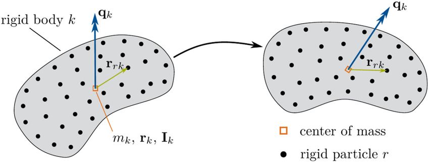
Fuchs et al. Adv. Model. and Simul. in Eng. Sci.(2021)8:15                                                              Page 10 of 33

                   discussed in the following and the reader is referred to the original publication [50].
                   Altogether, the acceleration ai = dui /dt of a particle i results from summation of all
                   acceleration contributions due to interaction with neighboring particles j and a body
                   force as

                                  1  2                ∂W              uij ∂W
                         ai =        (Vi + Vj2 ) −p̃ij      eij + η̃ij            + bi ,                        (15)
                                  mi                   ∂rij            rij ∂rij
                                       j

                   with volume Vi = mi /ρi of particle i, unit vector eij = ri − rj /|ri − rj | = rij /rij , relative
                   velocity uij = ui − uj , and density-weighted inter-particle averaged pressure and inter-
                   particle averaged viscosity

                                  ρj pi + ρi pj                  2ηi ηj
                         p̃ij =                    and η̃ij =           .                                       (16)
                                     ρi + ρj                    ηi + ηj

                   In the following, the acceleration contribution of a neighboring particle j to particle i is,

                   for ease of notation, denoted as aij , where ai = j aij + bi . The above given momentum
                   equation (15) exactly conserves linear momentum due to pairwise anti-symmetric particle
                   forces

                         mi aij = −mj aji ,                                                                     (17)

                   which follows from the property ∂W /∂rij = ∂W /∂rji of the smoothing kernel.

                   Equation of state
                   Following a weakly compressible approach, the density ρi and pressure pi of a particle i
                   are linked via the equation of state

                                                             ρi
                         pi (ρi ) = c2 (ρi − ρ0 ) = p0          −1                                              (18)
                                                             ρ0

                   with reference density ρ0 , reference pressure p0 = ρ0 c2 and artificial speed of sound c.
                   Note that this commonly applied approach can only capture deviations from the reference
                   pressure, i.e., pi (ρ0 ) = 0, and not the total pressure. To limit density fluctuations to an
                   acceptable level, while still avoiding too severe time step restrictions, cf. Eq. (41), strategies
                   are discussed in [21] how to choose a reasonable value for the artificial speed of sound c.
                   Accordingly, in this work the artificial speed of sound c is set allowing an average density
                   variation of approximately 1%.

                   Boundary and coupling conditions
                   Herein, both rigid wall boundary conditions as well as rigid body coupling conditions, are
                   modeled following [23]. In the former case, at least q = floor(rc / x) layers of boundary
                                                                               f
                   particles b are placed parallel to the fluid boundary D with a distance of x/2 outside
                   of the fluid domain f in order to maintain full support of the smoothing kernel. In the
                   latter case, rigid particles r of rigid bodies k are considered, while naturally describing the
                   fluid–solid interface  fs . In both cases, a boundary particle b or a rigid particle r contribute
                   to the density summation (14) and to the momentum equation (15) evaluated for a fluid
                   particle i considered as neighboring particle j. The respective quantities of boundary
Fuchs et al. Adv. Model. and Simul. in Eng. Sci.(2021)8:15 Page 11 of 33
Fig. 3 Orientation of a rigid body k with rigid particles r and their relative position rrk described via a unit
quaternion qk at different times
particles b respectively rigid particles r are extrapolated from the fluid field based on a
local force balance as described in [23]. Consequently, striving for conservation of linear
momentum, cf. Eq. (17), the force acting on a rigid particle r stemming from interaction
with fluid particle i, cf. Eq. (15), is given as
fri = −mi air . (19)
Remark 10 The floor operator is defined by floor(x) := max {k ∈ Z | k ≤ x} and returns
the largest integer that is less than or equal to its argument x.
Modeling the motion of rigid bodies discretized by particles
Within this formulation, each rigid body k is composed of several rigid particles r that are
fixed relative to a rigid body frame, i.e., there is no relative motion among rigid particles of
a rigid body. Thus, the rigid particles of a rigid body are not evolved in time individually,
but follow the motion of the rigid body described by the balance of linear and angular
momentum, cf. Eqs. (6)–(7). As a consequence of the spatial decomposition approach,
special communication between all processors hosting rigid particles r of a rigid body k
in terms of the evaluation of mass quantities, or resultant forces and torques, is required.
For ease of notation, in the following the index (·)s denoting solid quantities is dropped.
Orientation of rigid bodies
The orientation ψk of a rigid body k, described by one respectively three degrees of free-
dom in two- and three-dimensional space, is previously introduced without explicitly
defining a specific parameterization of the underlying rotation, e.g., via Euler angles or
Rodriguez parameters. Moreover, as stated in Remark 2, explicit evolution of the ori-
entation ψk requires special Lie group time integrators. A straightforward approach to
overcome aforementioned issues is to describe the orientation of a rigid body via quater-
nion algebra, cf. Remark 12. Consequently, in the following it is assumed that at all times
the orientation ψk of a rigid body k can be uniquely described by a unit quaternion qk ,
cf. Fig. 3. Once a local rigid body frame is defined, this allows to transform the relative
position of rigid particles rrk , cf. Remark 11, from that rigid body frame to the reference
frame, e.g., a global cartesian system.Fuchs et al. Adv. Model. and Simul. in Eng. Sci.(2021)8:15 Page 12 of 33
Remark 11 Note that the relative position of rigid particles rrk expressed in the rigid body
frame is, in general, a known (and constant) quantity, that only needs to be updated in
case the center of mass position rk changes, i.e., due to phase transitions.
Remark 12 For the sake of brevity, the principals of quaternion algebra are not delineated
herein. It remains the definition of operator ◦ denoting quaternion multiplication as used
in the following.
Parallel evaluation of mass-related quantities
In a first step, on each processor p the processor-wise mass p mk and center of mass
position p rk of a rigid body k are computed as
mr rr
p mk = mr and p rk = r (20)
r r mr
considering the mass mr and position rr of all affiliated rigid particles r being located in
the computational domain of processor p, cf. Fig. 4 for an illustration. Accordingly, the
processor-wise mass moment of inertia p Ik of a rigid body k follows componentwise (in
index notation) as
⎡ ⎡ ⎤ ⎤
p Ik,ij = ⎣Ir δij + ⎣ (p rk,q − rr,q )2 δij − (p rk,i − rr,i )(p rk,j − rr,j )⎦ mr ⎦ (21)
r q
with mass mr and mass moment of inertia Ir of a rigid particle r, cf. Remark 13, and
Kronecker delta δij , cf. Remark 14. The computed processor-wise quantities, i.e., mass p mk ,
center of mass position p rk , and mass moment of inertia p Ik , are communicated to the
owning processor of rigid body k. In a second step, on the owning processor the total
mass mk and center of mass position rk of rigid body k are computed over all processors p
as
p p mk p rk
mk = m
p k and r k = (22)
p p p mk
making use of the received processor-wise quantities. Similar to (21) the mass moment of
inertia Ik of rigid body k follows componentwise (in index notation) as
⎡ ⎡ ⎤ ⎤
Ik,ij = ⎣p Ik,ij + ⎣ (rk,q − p rk,q ) δij − (rk,i − p rk,i )(rk,j − p rk,j )⎦ p mk ⎦
2
(23)
p q
again considering the received processor-wise quantities. Finally, the determined global
quantities, i.e., mass mk , center of mass position rk , and mass moment of inertia Ik , are
communicated from the owning processor to all hosting processors of rigid body k.
Remark 13 The mass moment of inertia Ir of a rigid particle r with mass mr is com-
puted based on the effective volume Veff = ( x)d with initial particle spacing x.
In two-dimensional space (d = 2) assuming circular disk-shaped particles results in
√
Ir = 0.5mr reff with effective radius reff = x/ π. Accordingly, in three-dimensional
space (d = 3) assuming spherical-shaped particles results in Ir = 0.4mr reff with effective
√
radius reff = 3 0.75/π x.Fuchs et al. Adv. Model. and Simul. in Eng. Sci.(2021)8:15 Page 13 of 33
Fig. 4 Parallel distribution of a rigid body k with rigid particles r over several processors p illustrating the
evaluation of mass mk , center of mass position rk , and mass moment of inertia Ik via processor-wise
mass p mk , center of mass position p rk , and mass moment of inertia p Ik
Remark 14 The Kronecker delta δij used⎧ in Eqs. (21) and (23) to compute the mass
⎨1 if i = j ,
moments of inertia is defined by δij =
⎩0 otherwise.
Remark 15 The computation of the mass moment of inertia, cf. Eqs. (21) respectively (23),
is based on the Huygens-Steiner theorem, also called parallel axis theorem.
Parallel evaluation of resultant force and torque
To begin with, the resultant coupling and contact force acting on a rigid particle r of rigid
body k is given as
fr = fri + frr̂ (24)
i k̂ r̂
with coupling forces fri stemming from interaction with neighboring fluid particles i,
cf. Eq. (19), and contact forces frr̂ stemming from interaction with rigid particles r̂ of
contacting rigid bodies k̂, cf. Eq. (27). Similar to the computation of mass-related quantities
as described previously, the resultant force fk and torque mk acting on a rigid body k
are determined considering the parallel distribution of the affiliated rigid particles r on
hosting processors p, cf. Fig. 4. Thus, in a first step the processor-wise resultant force p fk
and torque p mk acting on rigid body k are computed as
p fk = fr and p mk = rrk × fr (25)
r r
with rrk = rr − rk while considering the resultant forces fr acting on all rigid particles r
being located in the computational domain of processor p. For correct computation of
the processor-wise resultant torque p mk the knowledge of the global center of mass
position rk is required on all processors. Finally, the computed processor-wise forces p fk
and torques p mk are communicated to the owning processor of rigid body k and summed
up to the global resultant force and torque acting on rigid body k
fk = p fk and mk = p mk . (26)
p pFuchs et al. Adv. Model. and Simul. in Eng. Sci.(2021)8:15 Page 14 of 33
Remark 16 In the case of a computation on a single processor, the evaluation of mass mk ,
center of mass position rk , and mass moment of inertia Ik of a rigid body k follow directly
from Eqs. (20) and (21), while the resultant force fk and torque mk directly follow from
Eq. (25), in each case without the need for special communication.
Contact evaluation between neighboring rigid bodies
For the modeling of frictionless contact between neighboring rigid bodies k and k̂, a
contact normal force law based on a spring-dashpot model, similar to [29], is employed.
The contact force is acting between pairs of neighboring rigid particles r and r̂ of contacting
rigid bodies, i.e., for distances rrr̂ < x with rrr̂ = |rrr̂ | = |rr − rr̂ |. Accordingly, the
contact force acting on a particle r of rigid body k due to contact with a particle r̂ of
neighboring rigid body k̂ is given as
⎧
⎨− min 0, kc (rrr̂ − x) + dc (err̂ · urr̂ ) err̂ if rrr̂ < x,
frr̂ = (27)
⎩0 otherwise,
with unit vector err̂ = rrr̂ /rrr̂ , stiffness constant kc , and damping constant dc . The min
operator in Eq. (27) ensures that only repulsive forces between the rigid particles are
considered, also known as tension cut-off.
Remark 17 Contact between a rigid body k and a rigid wall is modeled similar to Eq. (27)
considering rigid particles r of a rigid body k and boundary particles b of a discretized
rigid wall.
Remark 18 The applied contact evaluation between rigid bodies is for simplicity based
on a contact normal force law evaluated between rigid particles while neglecting fric-
tional effects. Generally, following a macroscopic approach of contact mechanics with
non-penetration constraint, the normal distance between the contacting bodies, typi-
cally determined via closest point projections, is the contact-relevant kinematic quantity.
Accordingly, the concept applied in this work, can be interpreted as a microscale approach
based on a repulsive/steric interaction potential [51] defined between pairs of rigid par-
ticles of contacting rigid bodies. In the current work, this approach has been chosen for
reasons of simplicity and numerical robustness. An extension to a macroscale approach,
i.e., a normal distance-based contact interaction [12,52,53], is possible in a straightforward
manner. In addition, also a momentum-based energy tracking method [54] was recently
applied for collision modeling of fully resolved rigid bodies [55,56].
Discretization of the heat equation using SPH
Thermal conduction in the combined fluid and solid domain governed by the heat equa-
tion (8) is discretized using smoothed particle hydrodynamics following a formulation
proposed by Cleary and Monaghan [57]
dTa 1 4κa κb Tab ∂W
cp,a = Vb (28)
dt ρa κa + κb rab ∂rab
b
with volume Vb = mb /ρb of particle b and temperature difference Tab = Ta −Tb between
particle a and particle b. The discretization of the conductive term is especially suited forFuchs et al. Adv. Model. and Simul. in Eng. Sci.(2021)8:15 Page 15 of 33
problems involving a different thermal conductivity among the fields [57]. In the equation
above, the index (·)φ with φ ∈ {f, s} for fluid and solid field is dropped for ease of notation.
Accordingly, the particles a and b may denote fluid particles i as well as rigid particles r,
respectively.
Modeling thermally driven reversible phase transitions
Due to the Lagrangian nature of SPH, each (material) particle carries its phase informa-
tion. This allows for direct evaluation of the discretized heat equation (28) for fluid and
rigid particles with corresponding phase-specific parameters of the particle a itself and of
neighboring particles b. Phase transitions in the form of melting of a rigid body occurs,
in case the temperature Tr of a rigid particle r exceeds the transition temperature Tt .
The former rigid particle r changes phase to become a fluid particle i. Conversely, phase
transitions in form of solidification occurs, in case the temperature Ti of a fluid particle i
falls below the transition temperature Tt and the former fluid particle i becomes a rigid
particle r.
Consequently, each time a rigid body k is subject to phase transition, its mass mk , center
of mass position rk , and mass moment of inertia Ik are updated. In addition, the velocity uk
after phase transition is determined based on quantities prior to phase transition indicated
by index (·) as
uk = uk + ωk × (rrk − rrk ) (29)
following rigid body motion with (unchanged) angular velocity ωk .
Time integration following a velocity-Verlet scheme
The discretized fluid and solid field are both integrated in time applying an explicit
velocity-Verlet time integration scheme in kick-drift-kick form, also denoted as leapfrog
scheme, that is of second order accuracy and reversible in time when dissipative effects are
absent [36]. Again, for ease of notation, in the following the indices (·)f and (·)s denoting
fluid respectively solid quantities are dropped. Altogether, for the fluid field the posi-
tions ri of fluid particles i are evolved in time, while for the solid field the center of mass
positions rk and the orientations ψk of all rigid bodies k are evolved in time. However, the
positions rr of rigid particles r are not evolved in time but directly follow the motion of
corresponding affiliated rigid bodies k.
In a first kick-step, the accelerations ain = (dui /dt)n , as determined in the previous time
step n, are used to compute the intermediate velocities
n+1/2 t n
ui = uin + a (30)
2 i
of fluid particles i, where t is the time step size. Similar, for rigid bodies k the linear and
angular accelerations akn = (d2 rk /dt 2 )n respectively αnk = (dωk /dt)n are used to compute
the intermediate linear and angular velocities
n+1/2 t n n+1/2 t n
uk = ukn + ak and ωk = ωnk + α . (31)
2 2 k
In a drift-step, the positions (and orientations) of fluid particles i and rigid bodies k are
updated to time step n + 1 using the intermediate velocities. Accordingly, the positionsFuchs et al. Adv. Model. and Simul. in Eng. Sci.(2021)8:15 Page 16 of 33
of fluid particles i follow as
n+1/2
rin+1 = rin + t ui (32)
and the center of mass positions of rigid bodies k as
n+1/2
rkn+1 = rkn + t uk . (33)
The orientations of rigid bodies k are updated making use of quaternion algebra. First, the
angular orientation increments from time step n to time step n + 1 are determined using
the intermediate angular velocities of rigid bodies k following
n+1/2
φn,n+1
k = t ωk . (34)
Next, the angular orientation increments are described by so-called transition quater-
nions qkn,n+1 . Finally, quaternion multiplication, cf. Remark 12, gives the updated orien-
tations of rigid bodies k at time step n + 1
qkn+1 = qkn,n+1 ◦ qkn . (35)
Once the updated orientations (and thus also the updated rigid body frames) are known,
n+1
the relative positions of rigid particles rrk can be transformed from the rigid body frame
to the reference frame. The velocities and the positions of rigid particles r are updated,
considering the underlying rigid body motion of the corresponding rigid bodies k, in
consistency with the applied time integration scheme following
n+1/2 n+1/2 n+1
urn+1/2 = uk + ωk × rrk and rrn+1 = rkn+1 + rrk
n+1
. (36)
n+1/2
Using the positions ran+1 and the intermediate velocities ua of fluid and rigid par-
n+1
ticles a ∈ {i, r}, the densities ρi of fluid particles i are computed via Eq. (14). The
densities ρr of rigid particles r are not evolved and remain constant. The temperature
rates (dTa /dt)n+1 of fluid and rigid particles a are then updated on the basis of Eq. (28)
with the temperatures Tan as well as the positions ran+1 and densities ρan+1 . Finally, the
temperatures of fluid and rigid particles a are computed as
n+1
dTa
Tan+1 = Tan + t . (37)
dt
The accelerations ain+1 of fluid particles i, cf. Eq. (15), and the forces frn+1 acting on rigid
particles r, cf. Eq. (24), are concurrently computed using the positions ran+1 , the interme-
n+1/2
diate velocities ua , and the densities ρan+1 of fluid and rigid particles a. Consequently,
the resultant forces fk and torques mkn+1 acting on rigid bodies k together with mass-
n+1
related quantities give the linear and angular accelerations akn+1 respectively αn+1 k , cf.
Eqs. (6) and (7). In a final kick-step, the velocities of fluid particles i at time step n + 1 are
computed as
n+1/2 t n+1
uin+1 = ui + a , (38)
2 iFuchs et al. Adv. Model. and Simul. in Eng. Sci.(2021)8:15 Page 17 of 33
while the linear and angular velocities of rigid bodies k are
n+1/2 t n+1 n+1/2 t n+1
ukn+1 = uk + a and ωn+1 = ωk + α . (39)
2 k k 2 k
Accordingly, the velocities of rigid particles r are determined following the motion of the
corresponding rigid bodies k to
urn+1 = ukn+1 + ωn+1
k
n+1
× rrk . (40)
To maintain stability of the time integration scheme, the time step size t is restricted
by the Courant–Friedrichs–Lewy (CFL) condition, the viscous condition, the body force
condition, the contact condition, and the conductivity condition, refer to [21,50,58,59]
for more details,
h h2 h mr ρcp h2
t ≤ min 0.25 , 0.125 , 0.25 , 0.22 , 0.1 ,
c + |umax | ν |bmax | kc κ
(41)
with maximum fluid velocity umax and maximum body force bmax .
Numerical examples
The purpose of this section is to investigate the proposed numerical formulation for solv-
ing fluid–solid and contact interaction problems examining several numerical examples
in two and three dimensions involving multiple mobile rigid bodies, two-phase flow, and
reversible phase transitions. To begin with, several numerical examples of a single rigid
body in a fluid flow, considering different spatial discretizations, are studied and com-
pared to reference solutions. In a next step, two examples close to potential application
scenarios of the proposed formulation in the fields of engineering and biomechanics are
investigated. Finally, the capabilities of the proposed parallel computational framework are
demonstrated performing a strong scaling analysis. The parameter values in the numerical
examples, unless indicated otherwise, are given in a consistent set of units and presented
in non-dimensional form.
Spatial discretization of a rigid circular disk
In the following, a rigid circular disk of diameter D = 2.5 × 10⁻³ with density ρ s =
1.0 × 10³ , motivated by two subsequent examples, is discretized with different values of
the initial particle spacing x. The mass ms and the mass moment of inertia I s (with
respect to the axis of symmetry) of the circular disk are computed with the proposed
formulation and shown in Fig. 5. With decreasing initial particle spacing x the values
for mass ms and mass moment of inertia I s converge to the analytical solution confirming
the proposed formulation. To illustrate, the resulting spatial discretizations of the circular
disk with rigid particles are shown in Fig. 6. Clearly, the approximation of the circular
shape of the disk is of better accuracy for decreasing initial particle spacing x. To keep
the computational effort at a feasible level, in the two subsequent examples the domain is
discretized with an initial particle spacing of x = 2.0 × 10⁻⁴ and x = 1.0 × 10⁻⁴ .Fuchs et al. Adv. Model. and Simul. in Eng. Sci.(2021)8:15 Page 18 of 33
Fig. 5 Spatial discretization of a rigid circular disk: mass ms and mass moment of inertia I s of a rigid circular
disk for different values of the initial particle spacing x (solid line) compared to the analytical solution
(dashed line)
Fig. 6 Spatial discretization of a rigid circular disk: resulting spatial discretization of a rigid circular disk with
rigid particles for selected values of the initial particle spacing x
A rigid circular disk floating in a shear flow
The following numerical examples are concerned with the motion of a rigid circular disk
floating in a shear flow. First, the principal setup of the problem along with numerical
parameters is described, thereafter, two distinct cases are considered in detail. For valida-
tion, the results obtained with the proposed formulation are compared to [8] also applying
SPH to discretize the fluid and the solid field.
A rigid circular disk of diameter D = 2.5×10⁻³ with density ρ s = 1.0×10³ is allowed to
move freely in a rectangular channel of length L = 5.0 × 10⁻² and height H = 1.0 × 10⁻² ,
cf. Fig. 7. The remainder of the channel is occupied by a Newtonian fluid with density ρ f =
1.0 × 10³ and kinematic viscosity ν f = 5.0 × 10⁻⁶ . The bottom and top channel walls
move with velocity uw /2 in opposite direction inducing a shear flow in the channel. The
Reynolds number of the problem is given as Re = uw D2 /4ν f H [8,60] taking into account
the diameter of the circular disk D and the channel height H. At the left and right end of
the channel, periodic boundary conditions are applied, cf. Remark 19.
For the fluid phase, an artificial speed of sound c = 0.25 is chosen, resulting in a reference
pressure p0 = 62.5 of the weakly compressible model. The background pressure pb of the
transport velocity formulation is set equal to the reference pressure p0 . The motion of the
bottom and top channel walls is modeled using moving boundary particles. The problem
is solved for different values of the initial particle spacing x for times t ∈ [0, 60.0] with
time step size t obeying respective conditions (41).
Remark 19 Imposing a periodic boundary condition in a specific spatial direction allows
for particle interaction evaluation across opposite domain borders. Moreover, particles
leaving the domain on one side are re-entering on the opposite side.Fuchs et al. Adv. Model. and Simul. in Eng. Sci.(2021)8:15 Page 19 of 33
Fig. 7 A rigid circular disk floating in a shear flow: geometry and boundary conditions of two different cases
Fig. 8 Migration of a floating rigid circular disk to the center line of a channel: vertical position ry and
horizontal velocity ux of the center of the floating circular disk in the channel computed with the proposed
formulation and an initial particle spacing of x = 2.0 × 10⁻⁴ (red dashed line) and x = 1.0 × 10⁻⁴ (black
solid line) compared to the reference solution [8] (crosses)
Case 1: Migration of a floating rigid circular disk to the center line of a channel
This case is based on studies [60,61] stating that a rigid circular disk floating in a shear
flow in a channel migrates to the center line of the channel independent of its initial
position and initial velocity. Herein, the rigid circular disk is initially at rest placed at
vertical position ry = 2.5 × 10⁻³ in the channel, cf. Fig. 7. The channel walls move in
opposite direction with a velocity magnitude of uw /2 = 0.01 resulting in the Reynolds
number Re = 0.625 of the problem.
The obtained vertical position ry and the horizontal velocity ux of the center of the
circular disk in the channel over time t are displayed in Fig. 8 for two different values of
the initial particle spacing x. The circular disk migrates to the center line of the channel
as expected, showing no significant difference between the results obtained with different
initial particle spacings x. In addition, a comparison to the results of [8] shows very good
agreement for the dynamics of the solution.
Case 2: Interaction of a floating rigid circular disk with a fixed rigid circular disk
In the presence of a rigid circular disk that is fixed at the center line of the channel, a
rigid circular disk floating in a shear flow migrates to a specific position of equilibrium
independent of its initial position and velocity as stated in [62]. Herein, the fixed and the
floating rigid circular disks are initially placed on the center line of the channel at horizon-
tal position rx = ±3.75 × 10⁻³ , cf. Fig. 7. The channel walls move in opposite direction
with a velocity magnitude of uw /2 = 0.012 resulting in the Reynolds number Re = 0.75
of the problem.Fuchs et al. Adv. Model. and Simul. in Eng. Sci.(2021)8:15 Page 20 of 33
Fig. 9 Interaction of a floating rigid circular disk with a fixed rigid circular disk: trajectory and horizontal
velocity ux of the center of the floating circular disk in the channel computed with the proposed formulation
and an initial particle spacing of x = 2.0 × 10⁻⁴ (red dashed line) and x = 1.0 × 10⁻⁴ (black solid line)
compared to the reference solution [8] (crosses)
Figure 9 shows the obtained trajectory, i.e., vertical position ry over horizontal posi-
tion rx , and horizontal velocity ux of the center of the floating circular disk in the channel
for two different values of the initial particle spacing x. The results obtained with initial
particle spacing x = 1.0×10⁻⁴ are in good agreement to the reference solution [8]. How-
ever, the results obtained with initial particle spacing x = 2.0 × 10⁻⁴ show fluctuations
of the horizontal velocity ux , which is why also the trajectory deviates from the reference
solution [8]. This can be explained with disturbances of the density field due to relative
particle movement [21], that are more pronounced with a coarser spatial discretization,
i.e., with larger initial particle spacing x.
A rigid circular disk falling in a fluid column
A rigid circular disk of diameter D = 2.5 × 10⁻³ with density ρ s = 1.25 × 10³ is initially
at rest placed on the y-axis at vertical position ry = 1.0 × 10⁻² in a closed rectangular
box of height H = 6.0 × 10⁻² and width W = 2.0 × 10⁻² , cf. Fig. 10. The remainder
of the box is occupied by a Newtonian fluid with density ρ f = 1.0 × 10³ and kinematic
viscosity ν f = 1.0 × 10⁻⁵ . A gravitational acceleration of magnitude |g| = 9.81 shall act
on both the fluid and solid field in negative y-direction. Following [8] this is modeled
considering the buoyancy effect, i.e., body force bs = (ρ s − ρ f )/ρ s g is acting on the solid
field while no body force bf = 0.0 is applied on the fluid field (each per unit mass). It
is worth noting that, naturally, it would also be possible to directly set the gravitational
acceleration for the fluid and solid field. For validation, the results obtained with the
proposed formulation are compared to [8] also applying SPH to discretize the fluid and
the solid field.
For the fluid phase, an artificial speed of sound c = 0.5 is chosen, resulting in a reference
pressure p0 = 250.0 of the weakly compressible model. The background pressure pb of
the transport velocity formulation is set equal to the reference pressure p0 . The stiffness
and damping constant applied for contact evaluation are set to kc = 1.0 × 10⁸ and
dc = 1.0 × 10² . The walls of the box are modeled using boundary particles. The problem
is solved for different values of the initial particle spacing x for times t ∈ [0, 0.8] with
time step size t obeying respective conditions (41).
The obtained vertical velocity and horizontal position of the center of the circular disk
in the box over time t are displayed in Fig. 11 for two different values of the initial particle
spacing x compared to the reference solution [8]. The results obtained with different
initial particle spacing x show only minor differences. The terminal velocity of the rigidFuchs et al. Adv. Model. and Simul. in Eng. Sci.(2021)8:15 Page 21 of 33
Fig. 10 A rigid circular disk falling in a fluid column: geometry and boundary conditions of the problem
Fig. 11 A rigid circular disk falling in a fluid column: vertical position ry and vertical velocity uy of the center
of the circular disk in the fluid column computed with the proposed formulation and an initial particle
spacing of x = 2.0 × 10⁻⁴ (red dashed line) and x = 1.0 × 10⁻⁴ (black solid line) compared to the
reference solution [8] (crosses)
circular disk is slightly smaller than given in the reference solution [8]. It shall be noted
that, in contrast to [8], contact of the rigid circular disk and the wall of the box is explicitly
considered. Consequently, the rigid circular disk comes at rest when approaching the
bottom wall of the box.
Melting and solidification of powder grains in a melt pool
In metal powder bed fusion additive manufacturing (PBFAM), structural components are
created utilizing a laser or electron beam to melt and fuse metal powder, layer per layer, to
form the final part. PBFAM has the potential to enable new paradigms of product design,
manufacturing and supply chains. However, due to the complexity of PBFAM processes,
the interplay of process parameters is not completely understood, creating the need for
further research, amongst others in the field of computational melt pool modeling [15,16].
For this purpose, an SPH formulation for thermo-capillary phase transition problems
with a focus on metal PBFAM melt pool modeling has recently been proposed [18]. For
simplicity, this and other state-of-the-art approaches [18–20] in the field consider powder
grains that are spatially fixed. In the real physical process, however, it is observed that,
depending on the processing conditions, melt evaporation and thereby induced vapor and
gas flows in the build chamber may result in powder grains entrainment and ejection, i.e.,
a considerable degree of material re-distribution during the melting process. On the one
hand, this effect considerably affects process stability and mechanisms of defect creation,
on the other hand, it can not be represented by state-of-the-art approaches restricted
to immobile powder grains [18–20]. In the following, a two- and a three-dimensional
example each with different geometry, boundary conditions, and material parametersYou can also read