Characterising optical array particle imaging probes: implications for small-ice-crystal observations
←
→
Page content transcription
If your browser does not render page correctly, please read the page content below
Atmos. Meas. Tech., 14, 1917–1939, 2021
https://doi.org/10.5194/amt-14-1917-2021
© Author(s) 2021. This work is distributed under
the Creative Commons Attribution 4.0 License.

Characterising optical array particle imaging probes: implications
for small-ice-crystal observations
Sebastian O’Shea1 , Jonathan Crosier1,2 , James Dorsey1,2 , Louis Gallagher3 , Waldemar Schledewitz1 , Keith Bower1 ,
Oliver Schlenczek4,5,a , Stephan Borrmann4,5 , Richard Cotton6 , Christopher Westbrook7 , and Zbigniew Ulanowski1,8,9
1 Department    of Earth and Environmental Sciences, University of Manchester, Manchester, UK
2 National  Centre for Atmospheric Science, University of Manchester, Manchester, UK
3 Department of Physics and Astronomy, University of Manchester, Manchester, UK
4 Particle Chemistry Department, Max Planck Institute for Chemistry, Mainz, Germany
5 Institute for Atmospheric Physics, Johannes Gutenberg University, Mainz, Germany
6 Met Office, Exeter, UK
7 Department of Meteorology, University of Reading, Reading, UK
8 Centre for Atmospheric and Climate Processes Research, University of Hertfordshire, Hatfield, UK
9 British Antarctic Survey, Natural Environment Research Council (NERC), Cambridge, UK
a now at: Max Planck Institute for Dynamics and Self-Organization, Göttingen, Germany

Correspondence: Jonathan Crosier (j.crosier@manchester.ac.uk)

Received: 30 June 2020 – Discussion started: 26 August 2020
Revised: 1 December 2020 – Accepted: 14 January 2021 – Published: 9 March 2021

Abstract. The cloud particle concentration, size, and shape        1   Introduction
data from optical array probes (OAPs) are routinely used to
parameterise cloud properties and constrain remote sensing
retrievals. This paper characterises the optical response of       A significant amount of our current understanding of cloud
OAPs using a combination of modelling, laboratory, and field       microphysics is based on in situ measurements made using
experiments. Significant uncertainties are found to exist with     optical array probes (OAPs). This includes how cloud proper-
such probes for ice crystal measurements. We describe and          ties are parameterised in numerical climate and weather mod-
test two independent methods to constrain a probe’s sam-           els and how they are retrieved from remote sensing datasets,
ple volume that remove the most severely mis-sized parti-          including global cloud and precipitation monitoring satel-
cles: (1) greyscale image analysis and (2) co-location using       lites such as NASA’s GPM (Global Precipitation Mission),
stereoscopic imaging. These methods are tested using field         CloudSat, and CALIPSO (Cloud-Aerosol Lidar and Infrared
measurements from three research flights in cirrus. For these      Pathfinder Satellite Observation) (Mitchell et al., 2018; Sour-
cases, the new methodologies significantly improve agree-          deval et al., 2018; Ekelund et al., 2020; Eriksson et al., 2020;
ment with a holographic imaging probe compared to con-             Fontaine et al., 2020).
ventional data-processing protocols, either removing or sig-          Optical array probes are a family of instruments that have
nificantly reducing the concentration of small ice crystals        been widely used by the cloud physics community for more
(< 200 µm) in certain conditions. This work suggests that the      than the last 40 years. Primarily OAPs have been operated
observational evidence for a ubiquitous mode of small ice          on research aircraft (Wendisch and Brenguier, 2013). They
particles in ice clouds is likely due to a systematic instrument   collect images of cloud particles and are used to derive cloud
bias. Size distribution parameterisations based on OAP mea-        particle concentration, size, and crystal habit (shape). Optical
surements need to be revisited using these improved method-        array probes operate by recording a shadow image as a parti-
ologies.                                                           cle crosses a laser beam that is illuminating a 1D linear array
                                                                   of photodiode detectors. If the light intensity at any of the
                                                                   detectors drops below a threshold value, the probe records

Published by Copernicus Publications on behalf of the European Geosciences Union.
1918                                                   S. O’Shea et al.: Characterising optical array particle imaging probes

an image of the particle and the corresponding timestamp. A         measured image size. Korolev et al. (1991) show that the
two-dimensional image of the particle is constructed by ap-         diffraction from spherical liquid drops can be approximated
pending consecutive one dimensional “slices” from the array         by the Fresnel diffraction from an opaque disc. The ratio of
of detectors as the particle moves perpendicular to the laser       the measured image diameter to the true particle diameter is a
beam due to the motion of air through the probe.                    function of the dimensionless distance from the object plane
   The rate at which data need to be acquired from the de-          Zd :
tectors depends on the air speed through the probe and the
required image resolution. For example, when operated on                   4λZ
                                                                    Zd =        .                                               (3)
research aircraft at a typical airspeed of 100 m s−1 , image                D02
slices from the detectors are acquired every 0.1 µs to achieve
an image resolution of 10 µm. Modern OAPs have 64- to 128-             Korolev (2007, hereafter K07) describe how the size of
element detector arrays with pixel resolutions ranging from         the bright spot at the centre of a diffraction image can be
10 to 200 µm. Monoscale probes use a 50 % drop in intensity         used to determine a sphere’s distance from the object plane
as a threshold for detection, which results in 1-bit binary im-     and therefore true size. O’Shea et al. (2019, hereafter O19)
ages (Knollenberg, 1970; Lawson et al., 2006), while most           show that this correction is effective for modern OAPs up to
greyscale OAPs have three intensity thresholds, which result        approximately Zd = 6, after which the images are too frag-
in 2-bit greyscale images (Baumgardner et al., 2001).               mented to reliably correct. O19 show that greyscale infor-
   When particles pass through the object plane of a probe,         mation can be used to remove these fragments by identifying
they are in focus and accurate digitised images are recorded.       the distance from the object plane of spherical particles in the
When particles are offset from this plane, the diffraction of       range Zd = 3.5 to 8.5. This allows a new DoF to be defined
light by the particle alters the size and shape of the recorded     that excludes the fragmented images.
image from its original form. When the distance from the               There has been significant discussion in the literature
object plane (Z) is sufficiently large, the reduction in light      about the presence of high concentrations of small ice parti-
intensity at the detector will no longer exceed the detection       cles (< 200 µm) observed by OAPs in cirrus and other types
threshold. This distance is known as the probe’s depth of           of ice clouds (Jensen et al., 2009; Korolev et al., 2011). O19
field (DoF). For large particle sizes, the DoF is constrained       show that fragmented images near the edge of the DoF have
by the physical separation between the laser transmit and re-       the potential to significantly bias OAP particle size distribu-
ceive optics, which are in protruding structures referred to as     tions (PSDs) and result in an artificially high concentration
“arms”. The following equation is generally used to define          of small particles.
the DoF of monoscale probes using a 50 % intensity thresh-             This paper quantifies the uncertainties in OAP size
old for detection (Knollenberg, 1970):                              and shape measurements of non-spherical ice crystals and
                                                                    presents corrections that remove large biases from OAP
          cD02                                                      datasets. In Sect. 3.1, 3D ice crystal analogues are repeti-
DoF = ±        ,                                         (1)
           4λ                                                       tively passed through the sample volume of an OAP at dif-
where D0 is the particle diameter, and λ is the laser wave-         ferent distances from the object plane. These results are used
length. c is a dimensionless constant, typically between 3          to examine the ability of a diffraction model based on angu-
and 8 (Lawson et al., 2006; Gurganus and Lawson, 2018).             lar spectrum theory to characterise the response of OAPs. In
The DoF is used to determine particle concentration, and as         Sect. 3.2 to 3.5 a variety of ice crystals from commonly oc-
a result uncertainty in c propagates into uncertainty in the        curring habits are tested with the diffraction model to quan-
derived concentration. Particle concentration can be calcu-         tify how OAP image quality degrades throughout a probe’s
lated by dividing the number of counts by the sample volume         sample volume. Section 4 suggests and tests methods to im-
(SVol), which is given by                                           prove OAP data quality. The impact these results have on ice
                                                                    crystal PSDs is examined using field measurements collected
              +DoF
              Z
                                                                   during three research flights in frontal cirrus. The impacts
SVol = TAS           R(E − 1) − D|| (Z) dZ,                  (2)    that OAP measurement bias has on our understanding of ice
            −DoF                                                    cloud microphysics are discussed in Sect. 5.
where TAS is the true air speed, E is the number of detector
array elements, R is the pixel size of the probe, and D|| is the    2     Methods
image diameter in the axis parallel to the optical array. The
integration of the effective array width (R(E − 1) − D|| (Z))       2.1    Optical array probes
is performed over whichever is smaller out of the DoF and
the arm width of the probe.                                         This paper uses data from two types of commercially avail-
   For spherical particles, corrections exist for the diffraction   able OAP: a CIP-15 (cloud imaging probe, DMT Inc., USA;
effects of sampling offset from the object plane, which al-         Baumgardner et al., 2001) and a 2D-S (2D stereo, SPEC Inc.,
lows for the calculation of the true particle size from the         USA; Lawson et al., 2006). The CIP-15 has a 64-element

Atmos. Meas. Tech., 14, 1917–1939, 2021                                              https://doi.org/10.5194/amt-14-1917-2021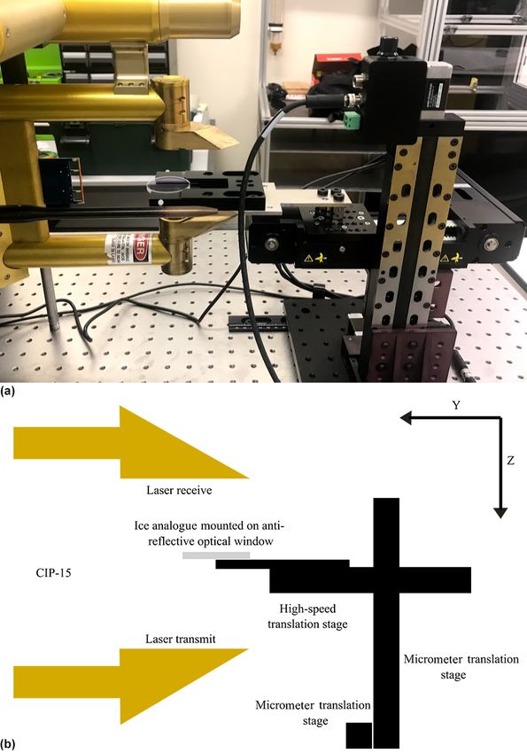
S. O’Shea et al.: Characterising optical array particle imaging probes                                                         1919

photodiode array and effective pixel size of 15 µm. The lab-
oratory experiments were conducted with a CIP-15 with an
arm separation of 70 mm (Sect. 3.1) and the field measure-
ments with a second CIP-15 with an arm separation of 40 mm
(Sect. 4.1). Images are recorded at three greyscale intensity
thresholds. For this work, they were set to the manufacturer
default settings of 25 %, 50 %, and 75 %. The 2D-S con-            Figure 1. Microscope images of sodium fluorosilicate crystals that
sists of two optical arrays and lasers orientated at right an-     were used as analogues for ice crystals. These are referred to as
gles to each other and the direction of motion of the par-         ROS118 (a), ROS250 (b), and ROS300 (c).
ticles and aircraft. The laser beams overlap at the centre
of the probe’s arms, and each pair of transmit and receive
arms are separated by 63 mm. Each optical array has 128 el-        2.2   Ice crystal analogues
ements and 10 µm pixel resolution. The 2D-S is a monoscale
probe with a single 50 % intensity detection threshold. Both       Three-dimensional ice crystal analogues were grown from
probes are fitted with anti-shatter tips to minimise ice shat-     a sodium fluorosilicate solution (Ulanowski et al., 2003).
tering on the leading edge of the probe during field mea-          These analogues have similar crystal habits to ice and a re-
surements. This was further minimised by removing particles        fractive index of 1.31, virtually identical to that for ice at
with inter-arrival times less than 1 × 10⁻⁵ s when calculating     visible wavelengths. Three rosette shapes were used in these
PSDs from field measurements (Field et al., 2006).                 experiments with approximate diameters 118 µm (ROS118),
   Baumgardner and Korolev (1997) show that the electronic         250 µm (ROS250), and 300 µm (ROS300) (Fig. 1). The CIP-
time response of older probes can significantly reduce the         15 was mounted as shown in Fig. 2 so that the laser beam
DoF of small particles. This effect has been minimised in          was vertically aligned. Each analogue was in turn placed on
more modern probes such as the 2D-S and CIP-15, which              an anti-reflective optical window that was attached to a three-
have an order of magnitude faster time response.                   axis translation system that allowed the analogue’s 3D posi-
   A range of definitions have been used to define the diame-      tion to be controlled. The stages that moved along the axes
ter of ice crystals from OAP images. Here we test three met-       parallel (x axis) to the diode array and laser beam (z axis)
rics that have been widely used by the community. First, the       each had a unidirectional position accuracy of 15 µm and
mean of the particle extent along the axes parallel and per-       travel ranges of 100 and 150 mm, respectively (X-LRM050A
pendicular to the optical array (mean X–Y diameter). Sec-          and Z-LRM150A, Zaber Technologies Inc., Canada). Move-
ond, the diameter calculated using D = (4A/π )1/2 , where A        ments along the axis that air flows through the probe un-
is the particle area calculated as the sum of the pixels (circle   der normal operation (y axis) were made using a belt-driven
equivalent diameter). Third, the major axis length of the el-      stage with a maximum speed of 1.1 m s−1 , positional accu-
lipse that has the same normalised second central moments          racy of 200 µm, and maximum travel range of 70 mm (X-
as the region (maximum diameter).                                  BLQ0070-EO1, Zaber Technologies Inc., Canada).
   An image frame from the OAP may contain more than                  CIP-15 images of the ice crystal analogues were collected
one object, where individual objects are defined as collec-        by moving them through the laser beam along the axis of air-
tions of pixels with eight-neighbour connectivity. This can        flow. For each analogue, this was repeated five times before
be due to diffraction, with a single particle appearing as more    its position was stepped in 0.5 mm increments between the
than one object as the structure and intensity of the transmit-    probe’s vertical arms (along the z axis). This allows images
ted light degrades due to poor focus. However, it may also         of the analogues to be compared at different distances from
be due to shattering causing multiple particles to have suffi-     the object plane.
ciently small separations that they are captured in the same          Images were post-processed to take account of any dif-
image frame or occasionally when there are very high con-          ference in velocity between the stage and the CIP-15 data
centrations of ambient particles. A particle sizing metric can     acquisition rate by resampling the images along the axis per-
either relate to the largest object in an image frame or use       pendicular to the optical array. This was performed to match
the bounding box encompassing all objects. Some previous           the aspect ratio at Z = 0 of the CIP-15 image and a micro-
studies have filled any internal voids within objects in an im-    scope image of each analogue. This typically corresponded
age frame. For this work, unless otherwise stated, the mean        to a particle stage velocity of ∼ 0.1 m s−1 .
X–Y , maximum, and circle equivalent diameters are calcu-
lated using the bounding box encompassing all objects in an        2.3   Synthetic data (angular spectrum theory)
image frame, and any internal voids are not filled.
                                                                   Theoretical shadow images of 2D non-spherical shapes were
                                                                   calculated using a diffraction model based on angular spec-
                                                                   trum theory (referred to as the AST model). Several previous
                                                                   studies describe this model in detail (Vaillant de Guélis et al.,

https://doi.org/10.5194/amt-14-1917-2021                                             Atmos. Meas. Tech., 14, 1917–1939, 2021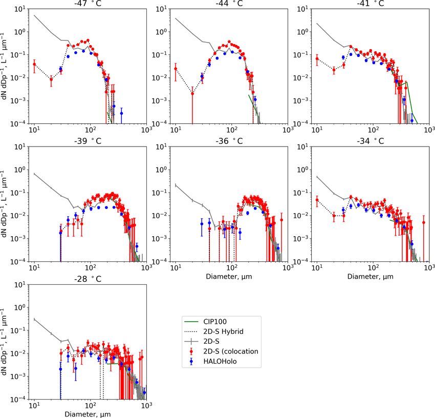
1920                                                     S. O’Shea et al.: Characterising optical array particle imaging probes

                                                                      ising the model with a variety of different ice crystal images.
                                                                      The ice crystal dataset contains 1060 images that were col-
                                                                      lected using a cloud particle imager (CPI, SPEC Inc., USA)
                                                                      and has previously been used to train habit recognition al-
                                                                      gorithms (Lindqvist et al., 2012; O’Shea et al., 2016). It in-
                                                                      cludes images of ice crystals from arctic, mid-latitude, and
                                                                      tropical clouds. These images have been manually classi-
                                                                      fied into seven habits (rosette, column/bullet, plate, quasi-
                                                                      spherical, column aggregate, rosette aggregate, and plate ag-
                                                                      gregate). To initialise the model, each CPI image was con-
                                                                      verted to a binary image. Shadow images were calculated
                                                                      every 2 mm for the range Z = 0 to 100 mm. These images
                                                                      were averaged to 10 µm pixel resolution, which is typical of
                                                                      modern OAPs. All simulations were performed using a light
                                                                      wavelength of 0.658 µm.
                                                                         An example simulation for a rosette crystal is shown in
                                                                      Fig. 3 and a column in Fig. 4; the top left panels show the im-
                                                                      ages at Z = 0 that are used to initialise the model. The other
                                                                      panels show images of the crystals at different distances from
                                                                      the object plane. Green, blue, and black pixels correspond
                                                                      to decreases in detector intensity of 25 % to 50 %, 50 % to
                                                                      75 %, and > 75 %, respectively. Figures 3 and 4 show the
                                                                      rapid deterioration in image quality within a few millimetres
                                                                      of the object plane, which will impact derived properties such
                                                                      as particle size, number, and habit. This compares to many
                                                                      tens of millimetres for the typical arm separation of modern
                                                                      OAPs.

                                                                      2.4   Aircraft measurements

Figure 2. (a) Image of the experimental set-up for the ice crystal    This paper uses measurements from three flights by the Facil-
analogue tests of the CIP-15. Panel (b) shows a schematic of the      ity for Airborne Atmospheric Measurements (FAAM) BAe-
experimental set-up. The CIP-15 is horizontally mounted on the left   146 research aircraft sampling frontal cirrus in the UK on
of the image. The translation stages used to move ice crystal ana-    the 11 March 2015 (nominal flight number B895), 7 Febru-
logues through the CIP-15 sample volume are shown on the right of     ary 2018 (C078), and 23 April 2018 (C097). The first two
the image. The x axis is perpendicular to the plane of drawing.       flights have previously been described in detail by O’Shea
                                                                      et al. (2016) and O19. For all three flights, the aircraft per-
                                                                      formed straight and level runs of approximately 10 min at dif-
2019a, b). We initialised the model using a 2D binary image           ferent temperatures within the cloud. Ice crystals were domi-
of an opaque shape at the object plane (Z = 0) and calculated         nated by rosettes, columns, and aggregates. Data from a 2D-S
the wave field for different positions between the probe arms         is available for the 11 March 2015 and CIP-15 for 7 February
in the z axis. This model has been shown to give good agree-          and 23 April 2018. On all flights the FAAM BAe-146 was fit-
ment with OAP images of several types of 2D rectangular               ted with a holographic imaging probe (HALOHolo). HALO-
columns using images printed on a rotating disc (Vaillant de          Holo has a 6576 × 4384 pixel CCD (charged-coupled device)
Guélis et al., 2019a).                                                detector with an effective pixel size of 2.95 µm and arm sepa-
   In this study, we use a variety of different shapes to ini-        ration of 155 mm. The probe acquires six frames per second,
tialise the model. In Sect. 3.1, the diffraction model is com-        which equates to a volume sample rate of ∼ 230 cm3 s−1 . The
pared to CIP15 images of 3D ice crystal analogues. To ini-            detection of small particles is limited by noise in the back-
tialise the model for the comparisons with ROS250 and                 ground image. Therefore, a minimum size threshold of 35 µm
ROS300, the CIP-15 image of them at Z = 0 is used. Due to             is applied, above which it is estimated that the probe’s detec-
the smaller size of ROS118 and coarse pixel size of the CIP-          tion rate is greater than 90 % (Schlenczek, 2017). Shattered
15, a microscope image of the analogue is used to initialise          particles were minimised by removing all particles with in-
the model. This image was converted to a binary image.                terparticle distances less than 10 mm (Fugal and Shaw, 2009;
   In Sect. 3.2 the quality of OAP images of commonly oc-             O’Shea et al., 2016).
curring ice crystal habits is explored. This is done by initial-

Atmos. Meas. Tech., 14, 1917–1939, 2021                                                https://doi.org/10.5194/amt-14-1917-2021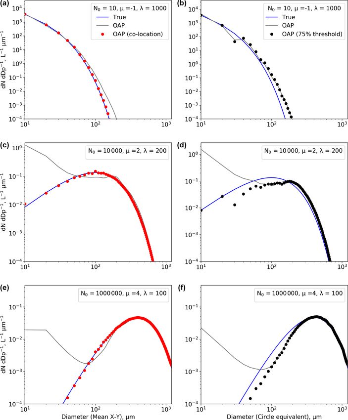
S. O’Shea et al.: Characterising optical array particle imaging probes                                                                      1921

Figure 3. Diffraction simulations from an image of a rosette crystal collected in cirrus cloud using a CPI (see text for details). Panel (a) shows
the image at Z = 0 that is used to initialise the model. The other panels show images at different distances from the object plane (Z = 5,
10, and 20 mm). Green, blue, and black pixels correspond to decreases in detector intensity of 25 % to 50 %, 50 % to 75 %, and greater than
75 %, respectively.

   Section 4.2 shows a comparison between the 2D-S and a                   the particle area is shown in the top right; both use a 50 %
cloud droplet probe (CDP, DMT Inc.) during a flight in liquid              drop in light intensity for the detection threshold. The other
stratus on 17 August 2018 (C031). The CDP sizes particles                  panels show different combinations of simple greyscale ra-
(3 to 50 µm) using the scattered light intensity assuming Mie              tios. The abbreviations A25–50 , A50–75 , and A75–100 are used
scattering theory and spherical particles (Lance et al., 2010).            to denote the number of pixels associated with a decrease in
The probe was calibrated during the campaign using glass                   detector signal of 25 %–50 %, 50 %–75 %, and 75 %–100 %,
spheres.                                                                   respectively. Example CIP-15 images of the ice crystal ana-
                                                                           logue ROS300 at three distance from the object plane are
                                                                           shown in Fig. 8.
3     Results and discussion                                                  All three analogues have a general trend of diameter ini-
                                                                           tially increasing with Z. The full DoF was sampled for
3.1    OAP and AST model comparison using ice crystal                      ROS118 and shows the images fragmenting and diameter de-
       analogues                                                           creasing near the edge of the DoF. In addition to these gen-
                                                                           eral trends, there is a significant amount of fine-scale struc-
This section compares CIP-15 images of ice crystal ana-                    ture that is specific to each sample. There is a general trend
logues with diffraction simulations using the AST model.                   of the greyscale ratio A75–100 decreasing with Z, while both
Figures 5–7 show the image size of the ice crystal analogues               A25–50 and A50–75 initially increase for all three analogues.
ROS118, ROS250, and ROS300 at different distances (Z)                      Like the diameter vs. Z plots, there is a significant amount of
from the object plane measured by the CIP-15 (black mark-                  fine-scale structure overlaying these general trends.
ers) and modelled using angular spectrum theory (red lines).                  In general, the AST model can capture the large-scale
Top left panels show the image diameter (mean X–Y ), while                 structure in these measured parameters, although some dis-

https://doi.org/10.5194/amt-14-1917-2021                                                       Atmos. Meas. Tech., 14, 1917–1939, 2021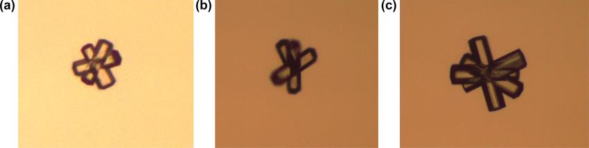
1922                                                  S. O’Shea et al.: Characterising optical array particle imaging probes

Figure 4. Same as Fig. 3 but for a column.

crepancies are present in the finer detail. For ROS118, the       tograms of D/D0 for each habit calculated for the Zd range
DoF from the experiments and the model agree to within            from 0 to 10.
±1 mm (Fig. 5). The size and greyscale parameters calcu-             Figure 9 shows large differences in these relationships
lated from CIP-15 images are not completely symmetrical           depending on whether the mean X–Y , maximum, or circle
about Z = 0. The reason for this is unclear; potential causes     equivalent diameters are used to define the particle size. For
are if the CIP-15 laser beam is not perfectly collimated, addi-   the 1060 ice crystal images used in this study, the median
tional refraction caused by the optical window used to mount      D/D0 over the Zd range from 0 to 8 is 1.1 using circle equiv-
the sample, or changes to the CIP-15 background or dark cur-      alent diameter, 1.0 using the mean X–Y diameter, and 1.0
rent calculation due to attenuation by the optical window.        using the maximum diameter. However, there is significantly
                                                                  less variability between crystals using circle equivalent diam-
                                                                  eter, which has an interquartile range D/D0 of 0.2 compared
3.2    OAP ice crystal sizing
                                                                  to 1.1 and 1.3 using the mean X–Y and maximum diame-
                                                                  ters, respectively. This is also shown in Tables S1–S3 in the
Having investigated the performance of the AST model us-          Supplement, which gives the median and interquartile range
ing 3D analogues of complex ice, we will now use the AST          D/D0 at selected Zd for each habit using the three different
model to examine the ability of OAPs to correctly deter-          size metrics.
mine the size of commonly occurring ice crystals. Figure 9           There is a general trend of increasing size with distance
left panels show the ratio of the measured diameter (D) to        from the object plane. Oversized estimations are up to ap-
the true diameter (D0 ) vs. Zd for diffraction simulations of     proximately 100 %, 200 %, and 50 % using mean X–Y , max-
1060 ice crystals. The data for each individual ice crystal are   imum, and circle equivalent diameters, respectively. How-
shown as grey lines, while the coloured lines are the median      ever, the degree of oversizing is dependent on habit, with
for each habit. Top panels show plots using the circle equiv-     quasi-spherical and plate aggregates most significantly over-
alent diameter, while the middle panels use the mean X–           sized using all D definitions. In agreement with O19, once D
Y diameter and maximum diameter. Right panels show his-

Atmos. Meas. Tech., 14, 1917–1939, 2021                                            https://doi.org/10.5194/amt-14-1917-2021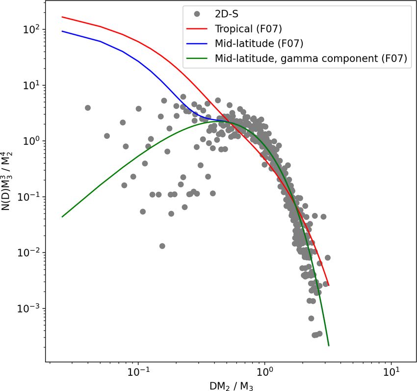
S. O’Shea et al.: Characterising optical array particle imaging probes                                                                 1923

Figure 5. A comparison between CIP-15 images and diffraction simulations (red lines) of the ice crystal analogue ROS118. Grey dots show
data from individual CIP-15 images, and black dots show the median for each 1 mm Z bin. Panel (a) shows the mean X–Y image diameter.
Panel (b) shows the number of pixels using 50 % detection thresholds. Other panels show the ratio of the number of pixels (area) at different
greyscale thresholds.

reaches a maximum, further increases in Z cause the images               their true particle diameter is shown as a function of Zd (left
to fragment and their size to decrease until they are no longer          panel), while probability density functions of D/D0 for each
visible.                                                                 habit are shown in the right panel. The median D/D0 for
   K07 use the size of the internal voids within images of               the Zd range 0 to 8 is 0.9, and the interquartile range is
droplets to determine their Zd and correct their size. O19               1.1. For a number of habits (rosette, plate, quasi-spherical,
show that this algorithm is effective using modern OAPs for              rosette aggregate, and plate aggregate), K07 reduce the num-
droplets with Zd < ∼ 6. For Zd > 6, the images are too frag-             ber of oversized particles across most of the DoF. For bullets,
mented for their size to be corrected. The K07 approach was              columns, and column aggregates, the K07 approach has min-
derived by considering Fresnel diffraction from opaque discs             imal impact on the probe sizing. For all habits, the K07 ap-
and has only been tested for images of spherical droplets.               proach is not able to remove the small image fragments that
However, in the absence of an alternative, previous studies              occur when a particle is near the edge of the DoF.
have applied K07 to images of ice crystals (e.g. Davis et
al., 2010). To examine the efficacy of this approach, Fig. 9             3.3   Depth of field dependence on particle habit
bottom panels show the mean X–Y diameter of the sim-
ulated images of ice crystals once the K07 approach has                  Uncertainty of derived physical quantities (e.g. number con-
been applied. The ratio of their K07 corrected diameter to               centration) from OAPs is dependent on the sample volume
                                                                         and therefore uncertainty in the DoF (see Eq. 2). The DoF of

https://doi.org/10.5194/amt-14-1917-2021                                                    Atmos. Meas. Tech., 14, 1917–1939, 2021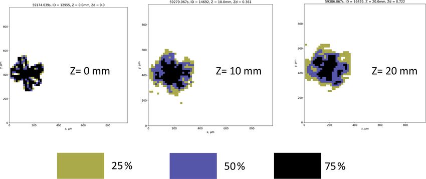
1924                                                    S. O’Shea et al.: Characterising optical array particle imaging probes

Figure 6. Same as Fig. 5 but for the ice crystal analogue ROS250.

an OAP is commonly calculated using Eq. (1) with a single c         circle equivalent diameter is used to define the particle size
value. The variable c in this equation is the Zd where a par-       compared to maximum and mean X–Y diameters.
ticle is no longer detected by the OAP. If a single c value is
used this would need to be independent of particle shape. Ta-       3.4   Greyscale information
ble 1 shows the median and interquartile range Zd where par-
ticles are no longer visible for each habit using the maximum,      Greyscale information in OAP imagery has previously been
mean X–Y and circle equivalent diameters. Using mean X–             used to filter severely mis-sized images and enforce a DoF
Y , the habit median DoF varies between Zd = 5.0 and 9.9            threshold that improves data quality (O19). Figure 10 shows
for rosettes and quasi-spherical particles, respectively. Using     combinations of simple greyscale ratios as a function of Zd
the maximum as the particle sizing metric, the median DoF           for the simulation of 1060 ice crystal images described in
varies by a similar amount ranging between Zd = 3.4 and 7.8         the previous section. Left panels use the size metric mean
for bullets and quasi-spherical crystals. In addition, particles    X–Y diameter in the Zd calculation, whereas the right pan-
have significant intra-habit variability using both maximum         els use circle equivalent diameter in the Zd calculation. Like
and mean X–Y , with most habits DoF interquartile ranges            the ratio D/D0 (Fig. 9), the greyscale ratios also show sig-
greater than 2 Zd . The variability is lower using circle equiv-    nificant variability between habits as a function of Zd . Fig-
alent diameter, with median DoFs ranging between 8.2 and            ure 10 shows this variability is greater if mean X–Y diameter
10.2 for plates and bullets, respectively, with habit interquar-    is used to calculate Zd , although it is still significant using
tile ranges near 1 Zd . As a result, derived physical quantities    circle equivalent diameter. The variability is larger still using
such as number concentration will have lower uncertainty if         maximum diameter (not shown).

Atmos. Meas. Tech., 14, 1917–1939, 2021                                              https://doi.org/10.5194/amt-14-1917-2021
S. O’Shea et al.: Characterising optical array particle imaging probes                                                      1925

Figure 7. Same as Fig. 5 but for the ice crystal analogue ROS300.

Figure 8. CIP-15 images of the ice crystal analogue ROS300 at three distances from the object plane.

https://doi.org/10.5194/amt-14-1917-2021                                                  Atmos. Meas. Tech., 14, 1917–1939, 2021
1926                                                       S. O’Shea et al.: Characterising optical array particle imaging probes

Figure 9. Left panels show the ratio of the measured diameter (D) to the true diameter (D0 ) vs. Zd for diffraction simulations of 1060 ice
crystals. The data for each individual ice crystal are shown as grey lines, while the coloured lines are the median for each habit. Right panels
show histograms of D/D0 for each habit calculated for the Zd range 0 to 10. Top panels show plots using the circle equivalent diameter,
while the middle panels use the mean X–Y and maximum diameters. Bottom panels show the diameter corrected using K07.

   The O19 approach uses simple greyscale ratios to deter-                3.5    Habit recognition
mine Zd for spherical liquid droplets near the edge of the
DoF (3.5 < Zd < 8.5). This allows a new DoF to be defined                 The shape of ice crystals is a key microphysical parameter
that excludes fragmented images, removing significant bi-                 impacting cloud radiative properties in several ways. A va-
ases in the PSD. This is possible since all spherical droplets            riety of automatic image recognition algorithms have been
independent of size have the same greyscale ratios at a given             applied to OAP datasets to classify particles into different
Zd . Figure 10 shows that this is not true for ice crystals               habits (Korolev and Sussman, 2000; Crosier et al., 2011; Praz
where the initial shape of the ice crystal has an impact on the           et al., 2018). These algorithms typically rely on geometrical
greyscale ratios at a given Zd . As a result, the O19 approach            features extracted from OAP images that have characteristic
cannot be used to determine Zd in the same way.                           values for specific habits. These characteristic values are usu-

Atmos. Meas. Tech., 14, 1917–1939, 2021                                                      https://doi.org/10.5194/amt-14-1917-2021
S. O’Shea et al.: Characterising optical array particle imaging probes                                                                    1927

Table 1. Median and interquartile range (IQR) normalised dimensionless distance from the object plane (Zd ) where particles are no longer
visible for different habits; this is equivalent to c in Eq. (1).

                                       Bullets     Column      Columns      Plates         Plate      Quasi-     Rosettes       Rosette
                                                 aggregates                           aggregates    spherical                aggregates
       Maximum             Median          3.4           4.6          3.9      5.6           5.8          7.8         4.6           4.1
                           IQR             1.3           1.5          2.0      2.8           1.9          2.0         1.9           1.9
       Mean X–Y            Median          6.8           6.6          7.2      7.0           7.0          9.9         5.0           5.4
                           IQR             2.0           1.7          2.1      3.0           2.4          2.0         2.0           2.0
       Circle equivalent   Median        10.2            9.4          9.9      8.2           9.0          9.4         8.6           9.2
       diameter            IQR            1.0            1.0          0.9      1.2           1.1          1.4         1.3           1.1

Figure 10. Combinations of number of pixels at different greyscale ratios as a function of Zd for the simulated ice crystal images. Panels (a),
(c), and (e) show plots where mean X–Y is used as the sizing metric, while panels (b), (d), and (f) use circle equivalent diameter.

https://doi.org/10.5194/amt-14-1917-2021                                                     Atmos. Meas. Tech., 14, 1917–1939, 2021
1928 S. O’Shea et al.: Characterising optical array particle imaging probes
rently the results of habit classification algorithms on OAP
datasets cannot be considered quantitative.
4 Methods to improve OAP size distributions
Depending on where in the sample volume a particle is ob-
served, the OAP image size can range between being as small
as a single pixel and up to twice the true particle diame-
ter (see Fig. 9). Algorithms such as those in K07 and O19
have been derived using spherical shapes and are therefore
not directly applicable to OAP PSDs of non-spherical shapes.
However, there are several possible approaches that could be
used to correct OAP ice crystal size distributions.
4.1 Greyscale filtering
Figure 11. The circularity (Eq. 4) of the rosette shown in Fig. 3 as
a function of distance from the object plane Z and Zd . Unlike for liquid droplets, the O19 approach does not accu-
rately determine Zd for non-spherical ice crystals. We now
describe a new technique to use greyscale information to re-
ally determined by manually classifying images into habits. move the most severely mis-sized ice crystals and constrain
These images are then used to set thresholds or train ma- the sample volume with a reasonable uncertainty using cir-
chine learning algorithms to automatically classify new im- cle equivalent diameter as the particle sizing metric. For ex-
ages. For example, Crosier et al. (2011) used the following ample, if the diffraction simulations are filtered to only in-
ratio to discriminate between ice crystals and liquid droplets: clude images that have at least one pixel with a greater than a
75 % drop in light intensity (Fig. 7), then the median position
P2 where particles are no longer visible (using a 50 % intensity
Circularity = , (4) threshold) is Zd = 4.6 (interquartile range 1.1 in Zd ). This
4π A
removes the fragmented images that begin to occur at ap-
where P is the particle perimeter, and A is the particle area proximately |Zd | > 6. The median ratio D/D0 for Zd < 4.6 is
including any internal void. Crosier et al. (2011) used a 1.2 (interquartile range = 0.1); however, particles may still be
threshold of 1.25 to discriminate between these two cate- oversized by approximately 40 % even with this filter applied
gories. When images are manually selected to train habit (Fig. 7). Other greyscale thresholds may be used to provide
recognition algorithms, only images that can be identified a more or less restrictive DoF constraint. Table 2 shows the
“by eye” as a specific habit will be included. For OAPs this median (interquartile range) c values for various greyscale
is likely to be images that are “in focus”. However, the shape thresholds between 65 % and 85 %. Using a 65 % threshold
of an OAP image and therefore the geometrical features that the median c value is 6.2 (interquartile range = 1.3), while for
are used in habit recognition algorithms depend on where 85 % it is 3.2 (interquartile range = 0.9). It should be noted
in the probe’s sample volume a particle is detected. For ex- that the lower the greyscale threshold, the higher the prob-
ample, Fig. 3 shows a simulated 190 µm rosette at different ability of a fragmented image being observed and the small
distances from the object plane. It is only in the top left panel particle concentration being biased.
(Z = 0) that it can be identified as a rosette from its image When determining the effective array width (Eq. 2), the
alone. Figure 11 shows how this particle’s circularity changes image size along the direction of the photodiode array should
with Z and Zd . At Z = 0 its circularity is near 4, while at be used. However, this size is a function of the particle’s Z
Z = 20 mm it is near 1 and may be confused with a spherical position, which is the reason why the effective array width
droplet. Figure 11 demonstrates that the measured particle needs to be integrated over the depth of field to determine
shape is highly dependent on the position in the sample vol- the sample volume (Eq. 2). This can be calculated using the
ume Zd (and Z) with the circularity decreasing by a factor 2 AST model if the true particle shape can be assumed (e.g.
by Zd = 1; in comparison the particle size has only changed spherical particles in liquid cloud). However, if the true par-
by 15 %. ticle shape is not known, as is often the case for ice clouds,
The variance in geometrical features for each habit will then it remains a source of uncertainty in the calculated sam-
not only be due to natural variability in the shape of ice ple volume.
crystals but also due to their position in the sample volume Figures 12 and 13 apply this new methodology to ambi-
when measured. To date, this second effect has not been ac- ent measurements collected during research flights in cirrus
counted for by habit recognition algorithms. Therefore, cur- on 7 February and 23 April 2018. Figure 12 shows PSDs
Atmos. Meas. Tech., 14, 1917–1939, 2021 https://doi.org/10.5194/amt-14-1917-2021S. O’Shea et al.: Characterising optical array particle imaging probes 1929
Table 2. Median (interquartile range) depth of field c value (Eq. 1) for 1060 ice crystal images using various greyscale intensity thresholds
and circle equivalent diameter. The median (interquartile range) ratio D/D0 for Zd < c is also given.
Greyscale intensity 65 70 75 80 85
threshold, %
c 6.2 (1.3) 5.4 (1.1) 4.6 (1.1) 4.0 (1.2) 3.2 (0.9)
D/D0 1.2 (0.1) 1.2 (0.1) 1.2 (0.1) 1.2 (0.1) 1.2 (0.1)
ever, it is possible that small particles could be misclassified
as artefacts or vice versa, and as a result HALOHolo could
either underestimate or overestimate the small ice concentra-
tion. For particles > 35 µm, it is estimated that the probe’s
detection rate is > 90 %, and previous work has shown ex-
cellent agreement with a CDP in liquid clouds (Schlenczek,
2017). However, HALOHolo PSDs should not be considered
the true PSD but rather another piece of evidence that sug-
gests for these cases OAPs overestimate small ice concentra-
tions using current data-processing techniques.
4.2 Stereoscopic imaging
A second method that could be used to constrain the DoF
Figure 12. Size distributions from the CIP-15 and HALOHolo for a of an OAP is to use the stereoscopic imaging that is pos-
run at −42 ◦ C on 7 February 2018. The black line shows the CIP-15 sible with the 2D-S. The 2D-S in effect consists of two
size distribution when images are filtered to only include those with OAPs (known as channels) orientated perpendicular to each
at least one pixel at the 75 % intensity threshold. other and the direction of motion of the particle and instru-
ment. Under normal operation the probe is oriented so that
one laser beam is horizontal and the other is vertical. The
from the CIP-15 and HALOHolo for a run at −42 ◦ C on two lasers overlap at the centre of each channel’s arms. As
7 February 2018 (16:02:00 to 16:10:00 GMT). This flight has well as increasing sampling statistics by having two chan-
previously been discussed by O19. Figure 13 shows equiva- nels which can be merged or averaged, this design also allows
lent PSDs for temperatures between −47 and −40 ◦ C col- some ice crystals to be viewed from two orientations to study
lected on 23 April 2018. For both probes, the particle diam- their aspect ratios. In this study we use this feature to con-
eter given is the circle equivalent diameter, and particles in strain the probe’s DoF, which greatly limits the magnitude
contact with the edge of the CIP-15 optical array have not of diffraction artefacts and represents the first implementa-
been included in the PSD calculation. The black lines show tion of stereoscopic analysis on an ambient OAP dataset. The
the CIP-15 size distribution when images are filtered to only 2D-S was designed so that Z = 0 on both channels is in the
include those with at least one pixel at the 75 % intensity region where the two lasers overlap. We refer to particles ob-
threshold. This threshold significantly reduces the concen- served by both channels as co-located particles. Co-located
tration of small particles (< 200 µm) compared to when this particles have tightly constrained Z position and should not
filtering is not applied (grey lines) and generally is in much be subject to significant mis-sizing due to diffraction. For the
better agreement with HALOHolo (a holographic imaging 2D-S, this is likely to be true for D0 > 20 µm. For a hypothet-
probe) (blue markers). This suggests that for these cases us- ical stereoscopic probe with larger optical arrays, it may be
ing current data-processing techniques, a significant fraction necessary to restrict the distance a particle can be from the
of the ice crystal number concentration at sizes < 200 µm is centre of the optical array.
an artefact due to optical effects. For the case where channel 0 is used for particle sizing
HALOHolo’s sample volume is not as strongly dependent and channel 1 is used to constrain the particle Z position, the
on particle size as it is for OAPs. However, as described ear- sample volume of co-located particles is given by
lier, measurements of small particles from HALOHolo are
limited by noise in the background image. For a complete SVol = TAS minimum cD 2 /2λ, ER (R (E − 1)
description of the HALOHolo data-processing and quality-
−DCH0 ) , (5)
control procedures, see Schlenczek (2017). HALOHolo uses
supervised machine learning to discriminate real particles where TAS is the true air speed, E is the number of array
from artefacts due to noise in the background image. How- elements, R is the resolution of the probe, D is the measured
https://doi.org/10.5194/amt-14-1917-2021 Atmos. Meas. Tech., 14, 1917–1939, 20211930 S. O’Shea et al.: Characterising optical array particle imaging probes Figure 13. Size distributions from the CIP-15 and HALOHolo for runs between −47 and −40 ◦ C on 23 April 2018. The black line shows the CIP-15 size distribution when images are filtered to only include those with at least one pixel at the 75 % intensity threshold. particle diameter, and DCH0 is the particle diameter measured Co-located particles could be confused with shattered par- along the axes of the channel 0 optical array. This requires ticles since they are also associated with short inter-arrival that particles in contact with the edge of the channel 0 optical times. Figure 14 (top panel) shows a histogram of inter- array have been removed. If channel 1 is used for particle arrival time for particles on the same channel for measure- sizing instead of channel 0, then particles in contact with the ments in cirrus on 7 February 2018. To minimise shattering edge of the channel 1 optical array are removed instead of events, each channel was independently filtered for particles channel 0, and DCH0 is replaced by DCH1 in Eq. (5). using an inter-arrival threshold of 1 × 10⁻⁵ s. It may still be For this method to be applicable, it is important to validate possible to mistakenly detect shattered particles as co-located that Z = 0 on both channels is in the laser overlap region. If particles if one shattering fragment splits into two particles, it is significantly offset this would prevent small co-located triggering each channel simultaneously but in spatially inde- particles from being observed, since the DoF from one chan- pendent parts of the sample volume. However, examination nel would not overlap with the optical array of the other chan- of co-located images suggest that this is rare. nel. Increasingly large offsets between the channels prevent To identify co-located particles, we use the difference in increasingly large co-located particles from being observed. arrival time between a particle on one channel and their clos- It is therefore important to check that this offset is not sig- est neighbour on the other channel. Figure 14 shows a his- nificant by regularly sampling in environments where small togram of co-location times for measurements in cirrus on particles are present (i.e. in liquid cloud or using a droplet 7 February 2018. This distribution is bimodal with a larger generator in a laboratory as in O19). mode centred at approximately 1 × 10⁻³ s and a smaller Atmos. Meas. Tech., 14, 1917–1939, 2021 https://doi.org/10.5194/amt-14-1917-2021
S. O’Shea et al.: Characterising optical array particle imaging probes                                                            1931

Figure 14. (a) Histograms of inter-arrival times for particles on the
same 2D-S channel for measurements in cirrus on 7 February 2018.        Figure 15. Example ice crystals observed by both channels of the
(b) A histogram of the difference in arrival time between a particle    2D-S. Images from channel 0 are shown in yellow and images from
on one channel and their closest neighbour on the other channel.        channel 1 are shown in blue.

mode at 1 × 10⁻⁷ s. The larger mode is associated with the              ume. These experiments with particle velocities of 1 m s−1
typical spatial separation between ambient particles, with its          resulted in a 1 × 10⁻⁵ s mode time delay in detection events
position dependent on the particle concentration. Examining             between the two channels of the 2D-S. This also corresponds
pairs of images from the smaller mode suggests that these               to an offset of 10 µm in the sample volume in the axis of air-
images are the same ice crystal viewed from different orien-            flow through the probe (y axis). These two sets of analysis
tations. Figure 15 shows example pairs of co-located images,            provide a robust independent verification of the spatial off-
with channel 0 images shown in yellow and channel 1 im-                 set between the two channels of the 2D-S. Therefore, when
ages shown in blue. In addition to overall consistency in the           considering ambient data, we classify co-located particles as
geometrical shapes between channel 0 and channel 1 images,              those with time separations less than 5 × 10⁻⁷ s.
there is also excellent consistency in the particle size along             Figure 16 shows a comparison between PSDs collected
the airspeed direction (x axis in Fig. 15) between these two            in liquid stratus cloud at 13 ◦ C on 17 August 2018. The
channels.                                                               grey lines show the 2D-S data for each channel using con-
   Figure 14 shows that most co-located particles do not trig-          ventional data-processing protocols without constraining the
ger both channels simultaneously within the time resolution             DoF, while the green and red lines show PSDs for just the co-
of the data acquisition system but are offset by a few hundred          located particles. The CDP is shown in blue. For this case,
nanoseconds. At 100 m s−1 data slices from the detectors are            no particles larger than approximately 200 µm are present.
acquired every 1 × 10⁻⁷ s, which corresponds to a spatial               All data-processing methods are in good agreement up to
separation of 10 µm. Using the laboratory droplet generator             100 µm. For larger sizes, the measurements using the co-
system described in O19, we were able to generate a con-                located particles are limited by counting statistics due to the
tinuous stream of droplets of known size, velocity, rate, and           low concentration of these particles. This illustrates the abil-
with precise control over the position within the sample vol-           ity of the 2D-S to detect small co-located particles.

https://doi.org/10.5194/amt-14-1917-2021                                                  Atmos. Meas. Tech., 14, 1917–1939, 2021
1932                                                    S. O’Shea et al.: Characterising optical array particle imaging probes

                                                                     idea of a suitable threshold, we will choose a size limit that
                                                                     prevents all particles with Zd > 2 from being included in the
                                                                     PSD. The maximum Z that the 2D-S can observe a parti-
                                                                     cle is Z = 31.5 mm (2D-S arm_width/2). This corresponds
                                                                     to a 222 µm particle at Zd = 2. However, since particles can
                                                                     be mis-sized by a factor 1.4, a size threshold of 300 µm is
                                                                     needed to ensure that no particle with Zd > 2 is included.
                                                                     Figure 17 (dashed lines) shows 2D-S PSDs processed using
                                                                     this hybrid approach.

                                                                     4.3    Other potential methods

                                                                     There are several other potential methods that could be
                                                                     used to improve OAP PSD measurements. First, reducing
                                                                     a probe’s arm width to physically limit a distance a parti-
                                                                     cle can be from the object plane would reduce out-of-focus
                                                                     particles. The amount the arm width would need to be de-
                                                                     creased depends on the level of mis-sizing that is deemed
                                                                     acceptable for a given particle size, with more accurate siz-
Figure 16. Size distributions from the 2D-S and CDP for different    ing and smaller particles requiring smaller arm widths. How-
temperatures during a research flight in liquid stratus on 17 Au-    ever, as well as decreasing the sample volume, reducing the
gust 2018 at 13 ◦ C. The grey lines show the 2D-S data using con-    probe’s arm width is likely to increase the proportion of shat-
ventional data-processing protocols without constraining the DoF,    tered artefact particles compared to ambient particles that the
while the green and red lines show size distributions for just the   probe measures, since shattered artefacts are thought to clus-
co-located particles. CDP size distributions are shown in blue.      ter near the probe’s arms.
                                                                        Second, statistical retrievals have been applied to parti-
                                                                     cle size distribution measurements where the instrument re-
   Figure 17 shows size distributions from the 2D-S                  sponse is a distorted version of the true ambient distribution.
and HALOHolo for different temperatures (averaged over               These methods are reliant on knowing or empirically ap-
∼ 10 min) during a research flight in cirrus on 11 March 2015        proximating the instrument function that distorts the ambient
(see O’Shea et al., 2016). The grey lines show the 2D-S data         distribution. These methods have been applied to OAP mea-
for each channel using conventional data-processing proto-           surements of spherical droplets (Korolev et al., 1998; Jensen
cols without constraining the DoF, while the red lines show          and Granek, 2002). For non-spherical particles, the distor-
size distributions for just the co-located particles. HALO-          tion function is dependent on the ice crystal habits present;
Holo size distributions are shown in blue. For all tempera-          therefore, the derived size distributions would have greater
tures, the conventional 2D-S data processing shows an ice            uncertainty, unless the particle shape is known a priori. How-
crystal mode at small sizes (< 200 µm). At warmer tempera-           ever, this methodology may still result in an acceptable level
tures (> −39 ◦ C) there is also a clear second mode at larger        of uncertainty if circle equivalent diameter is used, since its
sizes. However, these high concentrations of small ice parti-        intra- and inter-habit D/D0 (Zd ) variance is smaller than for
cles are not present in the co-located and the HALOHolo size         the mean X–Y and maximum diameters.
distributions. This suggests that using only co-located parti-
cles on the dual channel 2D-S probe is effective at remov-
ing significant biases at small particle sizes. At larger sizes      5     Implications for small-ice-crystal observations
(> 300 µm) the 2D-S data processing using conventional and
stereoscopic methods are in good agreement; however, the             In situ measurements of ice clouds have consistently ob-
latter method is limited by sampling statistics.                     served a mode in particle size distributions at small sizes
   Stereoscopic data processing has the advantage of remov-          (< 200 µm). This would imply that ice nucleation occurs at
ing out-of-focus artefacts that bias the PSD at small sizes,         all cloud levels, since small ice particles would rapidly grow
while at larger sizes traditional processing methods offer sig-      in regions of ice supersaturation or sublime in sub-saturated
nificantly improved sampling statistics. Therefore, a hybrid         regions. Particle shattering on the leading edge of a probe has
approach using stereoscopic processing for small sizes and           previously been identified as a possible explanation (Korolev
traditional processing methods for larger sizes is advanta-          and Isaac, 2005; Korolev et al., 2011). However, the impacts
geous. The choice of size threshold to switch between the            of shattering are thought to have been minimised by modi-
two methods is dependent on the arm width of the probe and           fying the leading edges of probes (Korolev et al., 2013) and
the level of mis-sizing that is deemed acceptable. To give an        using particle inter-arrival time algorithms (Field et al., 2006;

Atmos. Meas. Tech., 14, 1917–1939, 2021                                                https://doi.org/10.5194/amt-14-1917-2021
S. O’Shea et al.: Characterising optical array particle imaging probes 1933
Figure 17. Size distributions from the 2D-S and HALOHolo for different temperatures during a research flight in cirrus on 11 March 2015.
The grey lines show the 2D-S data using conventional data-processing protocols without constraining the DoF, while the green and red lines
show size distributions for just the co-located particles. The dashed black line shows a 2D-S processed using a hybrid of conventional and
co-location data processing (see text for details). HALOHolo size distributions are shown in blue.
Korolev and Field, 2015). Yet even with these improved mea- crystals observed in specific cirrus cloud cases (Figs. 12, 13
surements a small ice mode has been found to be ubiquitous and 17).
in ice cloud observations (McFarquhar et al., 2007; Jensen et To further explore the impact OAP mis-sizing has on
al., 2009; Cotton et al., 2013; Jackson et al., 2015; O’Shea et the measured PSD shape, we use the results from the AST
al., 2016). model. Consider the ambient ice crystal PSD N ( D 0 ) with
This work has shown that depending on where in the OAP units L−1 µm−1 . N ( D 0 ) is a 1-D array with E elements (the
sample volume a particle is observed its image size can be number of array elements). If this distribution is observed
as small as a single pixel or up to a 200 % overestimate of by an OAP with size-dependent sample volume SV ol ( D 0 )
the true particle diameter (see Fig. 9). Only a relatively small (units: L−1 s−1 , Eq. 2), then the number of ice crystals ob-
proportion of undersized larger particles are required to gen- served by the probe as a function of true particle diameter
erate a significant bias in number concentration at small sizes C ( D 0 ) (units: µm−1 s−1 ) is given by
(< 200 µm) due to the size dependence of the DoF (Eq. 1)
(O19). We have tested two methods that could be used to C (D 0 ) = N (D 0 ) SV ol ( D 0 ) . (6)
remove out-of-focus artefacts: greyscale filtering (Sect. 4.1)
and stereoscopic imaging (Sect. 4.2). Both methods either SV ol ( D 0 ) and C ( D 0 ) are both 1-D arrays with E el-
remove or significantly reduce the concentration of small ice ements. The symbol denotes Hadamard (element-wise)
multiplication. The number of ice crystals observed as a
https://doi.org/10.5194/amt-14-1917-2021 Atmos. Meas. Tech., 14, 1917–1939, 20211934 S. O’Shea et al.: Characterising optical array particle imaging probes
function of the measured diameter C ( D ) is given by the simulated OAP observations of this PSD, which have
a similar characteristic shape. The total particle concentra-
C (D) = M (D, D0 ) · C (D 0 ) , (7) tion observed by the simulated OAP over the size range 10
to 1280 µm is 3 % and 13 % higher than the true PSD us-
where M(D, D0 ) is an E×E array. Each column of M(D, D0 ) ing mean X–Y and circle equivalent diameters, respectively.
is the probability distribution that a particle of true size Figure 18 top left panel shows the PSD that a 2D-S would ob-
D0 has measured size D. These probabilities are depen- serve when only co-located particles are included (red mark-
dent on the particle shape, the particle sizing metric, probe ers). The total particle concentration from the co-located
characteristics (e.g. arm width, laser wavelength), and the PSD differs from the ambient distribution by less than 1 %.
data-processing protocols used (e.g. greyscale filtering, co- The total particle concentration when greyscale filtering is
location). The PSD observed by the probe N ( D ) (1-D array applied is 2 % lower that the true distribution.
with E elements) can then calculated by Figure 18 middle panels show an ambient distribution
with mode near 100 µm particles (µ = 2, λ = 200 cm−1 , and
N (D) = C (D) SV ol ( D ) . (8)
N0 = 1 × 10⁴ L−1 cm−1 ). The simulated OAP PSDs have
The symbol denotes Hadamard (element-wise) division. significantly different shapes with much higher concentra-
The probe arm width limits the maximum Zd that a parti- tions of particles < 100 µm. Here the OAP overestimates the
cle of given D0 can be observed. By choosing an arm width, total particle concentration over the size range 10 to 1280 µm
it is possible to calculate a probability distribution function by 74 % and 80 % using mean X–Y and circle equivalent di-
of possible D for each D0 from one of the D/D0 (Zd ) re- ameters, respectively. When stereoscopic imaging is used to
lationships shown in Fig. 9. For our example, we use an constrain the OAP sample volume (red lines), the small parti-
arm width of 70 mm and the median D/D0 (Zd ) relationship cle mode is removed. The true and simulated OAP total par-
for rosettes. We calculate M(D, D0 ) for two cases: when ticle concentration differ by < 1 %. Greyscale filtering again
mean X–Y and circle equivalent diameters are used as the removes the small particle mode but underestimates the total
particle sizing metric. To represent the true ambient distribu- particle concentration by 11 %.
tion, we use three different gamma distributions that all have Figure 18 bottom panels show an ambient PSD with
the form mode near 400 µm particles (µ = 4, λ = 100 cm−1 , and
N0 = 1 × 10⁶ L−1 cm−1 ); like the previous case the simu-
N (D) = N 0 D µ e−λD , (9) lated OAP PSD significantly overestimates the small particle
concentration. The simulated OAP PSD is bi-modal, while
where N is the number concentration. Figure 18 shows the true PSD is mono-modal. However, in this case the arti-
three combinations of the coefficients µ, λ (cm−1 ), and N 0 ficial small particles contribute a relatively small proportion
(L−1 cm−1 ). Left panels show plots using mean X–Y di- to the total number concentration in the 10 to 1280 µm size
ameter and the right panels show plots using circle equiv- range; as a result the simulated OAP only overestimates this
alent diameter. The ambient PSDs (blue lines) are com- by 4 % using both particle size metrics.
pared to simulated OAP observations using different data- A significant amount of our understanding of cloud mi-
processing methodologies. The grey lines represent an OAP crophysics is based on OAP measurements, with the small
with arm width of 70 mm using conventional data-processing particle artefact being present and manifesting in some man-
methods. The red markers represent a 2D-S using only co- ner. This includes how PSDs are parameterised in numerical
located particles, which has the effect of limiting the max- models and remote sensing retrievals. Generally in the litera-
imum Z a particle can be observed at to 0.64 mm. The ture some formulation of exponential or gamma function has
blue markers show simulated OAP measurements from a been used to represent ice crystal PSDs for observation or
greyscale probe with 70 mm arm width when the data have modelling studies (e.g. Cazenave et al., 2019; Delanoë et al.,
been filtered to only include particles that have at least one 2005, 2014; Field et al., 2007; Heymsfield et al., 2013; Mc-
pixel with a greater than 75 % decrease in light intensity. Farquhar and Heymsfield, 1997). These functions and the co-
It should be noted that these simulated distributions only efficients that are used in the literature all result in the highest
include mis-sizing due to diffraction and do not include ice crystal concentrations at the smallest sizes. For example,
other sources of OAP measurement uncertainty (e.g. count- Field et al. (2007) describe a parameterisation based on OAP
ing statistics). Counting statistics will be responsible for a measurements that is widely used by the passive and active
larger uncertainty for the co-located PSDs compared to con- remote sensing communities (e.g. Mitchell et al., 2018; Sour-
ventional data-processing methods. deval et al., 2018; Ekelund et al., 2020; Eriksson et al., 2020;
Figure 18 top panels show an ambient distribution (blue Fontaine et al., 2020). It describes a characteristic ice crystal
lines) dominated by small particles (µ = −1, λ = 1000 cm−1 , PSD that can be used to calculate moments of a PSD when
and N0 = 10 L−1 cm−1 ), with concentrations increasing with the ice water content is known. The functional form of the
decreasing size over the displayed size range 10 to 1280 µm, parameterisation consists of the summation of a gamma and
which is representative of modern OAPs. The grey lines show exponential distribution.
Atmos. Meas. Tech., 14, 1917–1939, 2021 https://doi.org/10.5194/amt-14-1917-2021You can also read