Particle size dynamics in abrading pebble populations - Earth Surface Dynamics
←
→
Page content transcription
If your browser does not render page correctly, please read the page content below
Earth Surf. Dynam., 9, 235–251, 2021
https://doi.org/10.5194/esurf-9-235-2021
© Author(s) 2021. This work is distributed under
the Creative Commons Attribution 4.0 License.

           Particle size dynamics in abrading pebble populations
                                 András A. Sipos1,2 , Gábor Domokos1,2 , and János Török1,3
             1 MTA-BME     Morphodynamics Research Group, Budapest University of Technology and Economics,
                                        Műegyetem rakpart 1–3, Budapest, Hungary
           2 Department of Mechanics, Materials and Structures, Budapest University of Technology and Economics,

                                        Műegyetem rakpart 1–3, Budapest, Hungary
                   3 Department of Theoretical Physics, Budapest University of Technology and Economics,

                                              Budafoki út 8, Budapest, Hungary
                                   Correspondence: András A. Sipos (siposa@eik.bme.hu)

                                   Received: 15 October 2020 – Discussion started: 31 October 2020
                         Revised: 20 February 2021 – Accepted: 23 February 2021 – Published: 26 March 2021

        Abstract. Abrasion of sedimentary particles in fluvial and eolian environments is widely associated with colli-
        sions encountered by the particle. Although the physics of abrasion is complex, purely geometric models recover
        the course of mass and shape evolution of individual particles in low- and middle-energy environments (in the
        absence of fragmentation) remarkably well. In this paper, we introduce the first model for the collision-driven
        collective mass evolution of sedimentary particles. The model utilizes results of the individual, geometric abra-
        sion theory as a collision kernel; following techniques adopted in the statistical theory of coagulation and frag-
        mentation, the corresponding Fokker–Planck equation is derived. Our model uncovers a startling fundamental
        feature of collective particle size dynamics: collisional abrasion may, depending on the energy level, either focus
        size distributions, thus enhancing the effects of size-selective transport, or it may act in the opposite direction by
        dispersing the distribution.

1     Introduction                                                   and with roughly similar axis ratios appear to be spatially
                                                                     close to each other. Size and shape segregation has been
1.1    Geological observations                                       broadly observed in various settings (Bird, 1996; Gleason
                                                                     et al., 1975; Hansom and Moore, 1981; Kuenen and Miglior-
Probably the most fundamental observation on pebbles is that         ini, 1950; Neate, 1967), and it was mostly attributed to the
they appear to be segregated both by size and shape, and it is       global transport of pebbles by waves (Lewis, 1931; Carr,
broadly accepted that the dynamics are driven by two phys-           1969) but, in some settings, may also be related to abrasion.
ical processes: transport and abrasion. Which of these pro-          Indeed, a detailed account of the interaction of abrasion and
cesses dominates may depend on the geological location and           transport is given by Landon (1930), who investigated the
also on timescales; however, geologists appear to agree that,        beaches on the west shore of Lake Michigan. He attributes
in general, neither process should be ignored.                       size and shape variation to a mixture of abrasion and trans-
   In coastal environments, one of the most remarkable ac-           port. Kuenen (1964) discusses Landon’s observations but dis-
counts of pebble size and shape distribution is provided by          agrees with the conclusions and attributes size and shape
Carr (1969) based on the measurement of approximately                variation primarily to transport. Carr (1969) observes dom-
100 000 pebbles on Chesil Beach, Dorset, England. In sum-            inant sizes and shape ratios emerging as a result of abra-
marizing his results, Carr provides mean values and sam-             sion and size grading, while Bluck (1967) describes beaches
ple variations for maximal pebble size and pebble axis ra-           in South Wales where equilibrium distributions of size and
tios along lines orthogonal to the beach. These plots reveal         shape are reached primarily by transport and abrasion plays
pronounced segregation by maximal size and shape; i.e., on           a minor role. Which of the two processes (transport or abra-
shingle beaches pebbles of roughly similar maximal sizes

Published by Copernicus Publications on behalf of the European Geosciences Union.
236 A. A. Sipos et al.: Particle size dynamics in abrading pebble populations
sion) dominate may well depend on the timescales they oper-
ate on. While abrasion appears in some scenarios to act much
more slowly than transport, a recent study (Bertoni et al.,
2016) verified mass losses on the order of 50 % on a pebble
beach over a 13-month period, indicating that in some set-
tings the two processes may indeed compete in determining
size and shape distributions.
In fluvial environments, while downstream fining of sedi- Figure 1. Schemes for (a) individual abrasion (Firey, 1974; Bloore,
ment has been often attributed to transport (Paola et al., 1992; 1977), (b) binary abrasion (Domokos and Gibbons, 2018), and
Ferguson et al., 1996; Fedele and Paola, 2007; Whittaker (c) collective abrasion. Volume loss only tracked for shaded parti-
et al., 2011), other authors have pointed to the significance cles. Arrows represent (non-simultaneous) collision events between
of attrition (Brewer and Lewin, 1993; Attal and Lavé, 2006; particles.
Dingle et al., 2017). In Miller et al. (2014) the authors, using
field data, provide quantitative assessment of the significance
of selective transport with respect to attrition in downstream collisions has been well understood and validated (Szabó
fining. Beyond the evolution of smooth size and shape distri- et al., 2013, 2015; Novák-Szabó et al., 2018). Still, despite
butions, there is yet another common phenomenon in fluvial the success of the Firey–Bloore geometric theory of shape
geomorphology where the interaction of transport and attri- evolution, it is clear (Domokos and Gibbons, 2018) that it is
tion could be far from trivial. The often observed presence not suited to predict the evolution of size: in stark contrast
of isolated large boulders in rivers (Huber et al., 2020) may with geological observations summarized in Sternberg’s law
be explained solely by transport, as these large pieces are of- (Sternberg, 1875), predicting exponential decay of particle
ten not carried by the river; rather, they move by a different mass and an infinite lifetime for all particles, geometric abra-
process (e.g., landslide or debris flow). On the other hand, sion theory predicted a finite lifetime for all particles. On the
these large rocks could also be interpreted as outliers emerg- other hand, Sternberg’s broadly accepted theory of mass evo-
ing spontaneously in a pebble size distribution on which col- lution (Sternberg, 1875) had nothing to offer regarding the
lisional abrasion certainly has strong impact in upper reaches evolution of shape. Recognizing this challenge, in Domokos
of rivers. and Gibbons (2018) a unified theory, called volume-weighted
As we can see, both in coastal and fluvial environments it shape evolution, has been proposed which, on one hand, re-
is a generally accepted fact that the two processes (transport produces all the geometric features of the Firey–Bloore geo-
and attrition) appear to compete in shaping the evolution of metric theory and, on the other hand, also predicts mass evo-
pebble shape and pebble mass distributions. How exactly this lution in accordance with Sternberg’s law.
competition may play out and in what manner attrition may
contribute to this process is the subject of our paper. 1.2.2 Binary abrasion
We also remark that while all available observations in-
The first stepping stone between the theory of individual
dicate that attrition could be a relevant factor in the evolu-
abrasion and collective abrasion is the model for mutual,
tion of shape and mass distributions, so far, in the absence of
binary abrasion, where two particles mutually abrade each
any predictive theory, no datasets have been collected which
other, and we track both evolutions (see Fig. 1b). In this case
would allow verifying any theoretical predictions. We will
one can still write mean field equations by averaging over
point out potential strategies for verification in Sect. 4.
many collisions, and the mass and shape evolution of both
particles are recorded. For any binary abrasion model of size
1.2 Existing theory evolution, we postulate the following requirements:
1.2.1 Individual abrasion – size evolution should follow Sternberg’s law,
Individual abrasion is a theory describing the mass and shape – mass loss in a collision should be a monotonically in-
evolution of one individual particle (abraded particle) un- creasing function of collision energy, and
der the impacts of many incoming particles (abraders) (see – the model should be fully compatible with the geometric
Fig. 1a). In the mean field theory for the geometry of indi- evolution model.
vidual abrasion only the mass and shape of the abraded par-
ticle is recorded; the effect of impacts is averaged and the The unified theory in Domokos and Gibbons (2018) of-
evolution is determined by the size of the abraded particle fers a model satisfying all three requirements: by extending
compared to the average size of the abrading particles. the Firey–Bloore equations and Sternberg’s theory and us-
Since the seminal papers by Firey (1974) and Bloore ing the kinetic energy of collision, models for binary shape
(1977), the mean field geometric theory of individual abra- evolution and for binary mass evolution of two mutually
sion (i.e., shape evolution) for sedimentary particles under abrading particles were put forward. These two models have
Earth Surf. Dynam., 9, 235–251, 2021 https://doi.org/10.5194/esurf-9-235-2021A. A. Sipos et al.: Particle size dynamics in abrading pebble populations 237
been merged in Domokos and Gibbons (2018) into a uni-
fied volume-weighted theory of binary abrasion, compatible X1+r Y 1−r
Xt = −c12 , (3)
both with the Firey–Bloore and with the Sternberg theory. X+Y
The volume-weighted model for binary mass evolution, de- Y 1+r X1−r
scribing the time evolutions for the masses X(t), Y (t) of two Yt = −c21 . (4)
X+Y
particles with respective material properties m1 , m2 can be
written as Note that these equations are identical to the formulas (118)
and (119) in Domokos and Gibbons (2018) with α = 0 in
XY their notation and taking r = ν, X = VX , Y = VY , c12 =
Xt = −c12 , (1)
X+Y c21 = c. Alternative interpretations of r are also possible; we
YX will discuss the role of the environmental parameter r in de-
Yt = −c21 , (2)
X+Y tail in Sect. 2.4. Henceforth, in the main body of this paper
(apart from Appendix A) we assume that the pebble popu-
where the subscript t refers to differentiation with respect
lation is homogeneous, i.e., that the material for all pebbles
to time and the constant prefactors c12 and c21 , which we
is identical so we have c = c12 = c21 and the sole role of the
call the binary abrasion parameters, depend simultaneously
constant c is to set the timescales. We will incorporate this
on the materials m1 and m2 of the X and Y particles, respec-
into the time variable t, and, henceforth, for homogeneous
tively.
pebble populations, we set c ≡ 1. We will discuss the role and
We also note that in the case of two identical particles
identification of material constants in heterogeneous pebble
(e.g., two particles with identical masses X = Y and identi-
populations in Appendix A.
cal material properties cXY = cY X ) the system (Eqs. 1 and 2)
Once the kernel has been established, we make the as-
predicts mass evolution according to Sternberg’s law. In the
sumption that for large N the collective size evolution is
case of different masses or properties we still have an infi-
a stochastic process driven by many binary events among
nite lifetime, with one of the particles approaching zero mass
the particles, implying that the core of the collective pro-
asymptotically as time goes to infinity and the other particle
cess is still the abovementioned collision kernel. This allows
approaching a finite mass.
for the construction of the master equation, also known as
the Fokker–Planck equation, which describes the time evo-
1.2.3 Collective size dynamics lution of the particle size distribution. Although the collec-
Independently of individual (and binary) abrasion theory tive abrasion is a stochastic process, in the N → ∞ limit the
there exists broad interest in collective shape and size evo- collision kernel will uniquely determine the global evolution
lution models tracking mutually colliding populations of N of the continuous size distribution. The master equation (or
particles (see Fig. 1c). Similar problems arise in particular Fokker–Planck equation) expresses this evolution. Determin-
in the context of coagulation (da Costa, 2015) and dynamic ing the master equation based on the collision kernel is the
fragmentation processes (Cheng and Redner, 1988). In such second step in the statistical model.
collective evolution models the main question is how the size
distribution of particles, starting from an initial distribution, 1.3 Our model
evolves in time due to the mutual collisions. These models
1.3.1 Relationship to earlier models
use a standard framework relying on a so-called collision ker-
nel. In a more general setting, the collision kernel is referred The above-outlined structure is characteristic of coagula-
to as the interaction kernel. Our choice of terminology is mo- tion fragmentation models (da Costa, 2015), in particular for
tivated by the fact that in our case the only interactions are non-linear fragmentation, which describe fragmentation pro-
collisions. cesses triggered by binary collisions of particles. Our model
The collision kernel can be derived from the binary equa- may be regarded as a special case of the non-linear fragmen-
tions (the physical model of the N = 2 case) by incorporating tation models (Cheng and Redner, 1988) since, in addition
statistical effects, i.e., that collision probability may depend to the standard framework adopted in these models, we also
on particle speed or mass. In Domokos and Gibbons (2018) make two simplifying assumptions:
the binary model (Eqs. 1 and 2) was extended to a kernel
by introducing an additional scalar parameter r (to which we 1. we only consider collisions where the relative mass loss
will also refer as the environmental parameter of the evolu- is small (i.e., the particles lose only fragments with
tion), representing the assumption that on average, only the small relative mass), and
collision probability depends on particle size and the colli- 2. the small fragments generated in the collisions are not
sion speed is independent of mass: considered further in the evolution.
By implementing these two assumptions into the statisti-
cal model based on the collision kernel (Eqs. 3 and 4), we
https://doi.org/10.5194/esurf-9-235-2021 Earth Surf. Dynam., 9, 235–251, 2021238 A. A. Sipos et al.: Particle size dynamics in abrading pebble populations
take the first step towards establishing the statistical theory
of collective size and shape evolution of sedimentary parti-
cles. This approach offers multiple methodological advan-
tages. On one hand, by using Eq. (4) as the collision kernel,
our statistical model will be compatible with Sternberg’s law,
so we can expect the collective evolution also to observe this
theory, albeit in a statistical sense. On the other hand, we can
also expect all our results to be compatible with an extended
(future) theory which also describes collective shape evolu-
tion based on the unified, volume-weighted geometric theory
in Domokos and Gibbons (2018).
Figure 2. Schematic description of the evolution of mass distri-
1.3.2 Basic notations
bution of a pebble population: in a dispersing process the relative
To describe our construction we will need to address both the size variation R(t) of the mass distribution, either represented by an
size evolution of individual particles (under the collision ker- empirical histogram (Carr, 1969) or a continuous function (f0 (x))
nel) as well as the evolution of size distributions. While parti- at t = 0, increases. In the continuum model of a focusing process
R(t) decreases as time evolves; however, in a discrete model with a
cle size appears in both settings, we need to distinguish care-
finite number of particles some outliers appear (indicated by dashed
fully: in individual and binary models particle size evolves in
ellipse) with mass substantially above the average. The reduced dis-
time; in collective models size distribution evolves in time. tribution (without the outliers) produces a decreasing relative vari-
As a consequence, in the individual setting the variable de- ance, analogous to the continuous model.
noting size may be differentiated with respect to time; in the
collective setting this is not the case. We will use X, Y to de-
note individual particle sizes (either volume or mass) and we cesses belonging to this regime will thus amplify the
will use x, y to denote the independent variables of size dis- segregating effects of size-selective transport.
tributions. The time evolution of individual particle size will
be denoted by X(t), Y (t) with time derivatives Xt (t), Yt (t) – For r < 0.5 we find dispersing processes with increas-
(arguments of a function written in subscript will refer to dif- ing R(t), thus counteracting size-selective transport
ferentiation throughout the paper). The time evolution of size processes. This corresponds to collisional abrasion at
densities will be denoted by f (x, t), f (y, t) with time deriva- higher energy levels.
tives ft (x, t), ft (y, t) and size derivatives fx (x, t), fy (y, t).
As collisional abrasion may occur within a broad range
We denote the expected value and variance of these size dis-
of energies, these two basic scenarios of the model (illus-
tributions, respectively, by E(t) and W (t) and we will pri-
trated in Fig. 2) offer an explanation for the broad range of
marily use the relative variance R(t) = W (t)/E(t)2 to char-
geological observations (Bluck, 1967; Landon, 1930; Carr,
acterize the evolution of the distributions.
1969; Kuenen, 1964) in relating the relative significance of
transport and abrasion in various scenarios. Our model also
1.3.3 Main results reflects the universality of Sternberg’s law by predicting, re-
gardless of the environmental parameter r, exponential decay
The collision kernel (Eqs. 3 and 4) for mass evolution in as the universal evolution E(t) of the expected value.
Domokos and Gibbons (2018) has one single environmental In general, the evolution equations generated by Eqs. (3)
parameter r, which is inherited by the corresponding Fokker– and (4) for the mean E(t) and the variance W (t) are integro-
Planck equation (shown in Sect. 2.2). As we will describe differential equations which are hard to solve analytically.
in Sect. 2, the environmental parameter r may, depending To support our claims, we will use three types of approxima-
on interpretation, represent either the size dependence of the tions:
number of collisions or, alternatively, the size dependence of
collision energy. Regardless of the interpretation, in Sect. 2.3 a. We approximate the kernel (Eqs. 3–4) by its truncated
we find that the value r = 0.5 is critical as it separates two Taylor series expansion and investigate the evolution of
regimes of collective abrasion with a qualitatively different general initial density functions. This is found in Ap-
evolution R(t) of the relative variance: pendix C1.
– For r > 0.5 we find focusing processes with decreas- b. We regard the full kernel; however, we only investigate
ing R(t), approaching R(t) = 0 in the limit as time ap- density functions obtained as a small perturbation of the
proaches infinity. Here the size distribution converges Dirac delta (i.e., populations of almost identical parti-
to a Dirac-delta function. This parameter range corre- cles). This is done in Appendices C2 and C3.
sponds to lower energy levels. Natural abrasion pro-
Earth Surf. Dynam., 9, 235–251, 2021 https://doi.org/10.5194/esurf-9-235-2021A. A. Sipos et al.: Particle size dynamics in abrading pebble populations 239
c. We numerically compute both the discrete and the con- The above simple procedures apply only for homogeneous
tinuum models. For details see Sect. 3. populations. We lay out the procedures for the testing of the
model for heterogeneous populations in Appendix A, where
We will briefly refer to the first two approximations as the we also perform partial testing for the laboratory data ob-
continuum model. In the case of the third approximation we tained by Attal and Lavé (2009).
do direct, discrete simulations of finite particle populations;
we use the full kernel and we call this the discrete model.
One startling feature of the latter (as compared with the for- 2 Modeling collective size dynamics
mer) is the appearance of outliers, i.e., particles substantially
2.1 General form of the collision kernel
larger than the vast majority (illustrated in Fig. 2). As we can
observe, the bulk of the density function closely mimics the The first simplification described in Sect. 1.3.1 implies that
evolution in the continuum model. The quantitative analogy the limit where relative fragment mass approaches zero of-
in the evolution of the relative variation R can also be re- fers a good approximation; thus it permits a collision kernel
covered if we consider a reduced density function f ∗ (t1 , x) of the type used in Ernst and Pagonabarraga (2007), describ-
by omitting the outliers, i.e., by applying an upper cutoff in ing continuous mass evolution via coupled ordinary differen-
size, omitting bins containing only one particle. The reduced tial equations for the evolution of particles with masses X(t)
density function f ∗ (t1 , x) is characterized by the reduced rel- and Y (t):
ative variation R ∗ , which will decrease in a focusing process;
however, in contrast to the continuum model, it will not ap- − Xt = ψ 1 (X, Y ), (5)
proach zero but a positive constant. 2
− Yt = ψ (X, Y ), (6)
1.4 Testing of the model for homogeneous pebble where ψ 1 (X, Y ) and ψ 2 (X, Y ) are differentiable (C 1 ) func-
populations tions, with positive values (i.e., R+ × R+ → R+ ). Symmetry
of the binary process implies ψ 1 (X, Y ) = ψ 2 (Y, X), so often
As outlined above, our model is defined on two levels: the superscripts are suppressed and the kernel is simply referred
collision kernel (Eqs. 3–4) we will briefly refer to as the in- to as ψ(., .). Selection of the kernel encapsulates not only the
put level as it defines the basic physics of the underlying col- physics of binary collisions, it also may include the mass-
lisions. The Fokker–Planck equation we will briefly refer to dependent probability of collision between two particles. We
as the output level as it defines the evolution of the mass den- will discuss the identification of physically sound kernels in
sity function based on the collision kernel. One may test the Sect. 2.3.
model at both levels. Below we discuss the case of homo-
geneous pebble populations where the evolution of the mass 2.2 General form of the master equation
distribution is controlled by the single material parameter c
and the single environmental parameter r: The second simplification in Sect. 1.3.1 permits the construc-
tion of the master equation solely based on the collision ker-
a. One may test the model at the input level, by fitting the nel (by omitting additional terms for the remainder of the
kernel (Eqs. 3–4) to laboratory tests where the abrasion fragmented material). These simplifying assumptions also
rate is plotted as a function of particle size. Such an ex- set our model apart from general fragmentation models in
periment could be used to determine the material pa- another respect: in the latter, constant mass is prescribed as a
rameter c for a given homogeneous population. Also, if global time invariant while the (integer) number of particles
the laboratory test imitates the environment of the natu- changes, whereas in our model total mass decreases while the
ral process, the environmental parameter r may also be number of particles remains constant and serves as a global
obtained in this manner. We also note that the functional invariant.
relationship between particle size and abrasion rate will Using these considerations, for our problem the master
not only depend on the parameters but also on particle equation is found to be
size. For details, see Appendix A.
Z∞
b. One may test the model at the output level by measuring ∂
ft (t, x) = f (t, x) f (t, y)ψ(x, y)dy
the time evolution of full mass distributions and fitting ∂x
0
the respective material and environmental parameters c
and r to this dataset. While we are not aware of any such Z∞
public dataset, this could be performed in a laboratory = fx (t, x) f (t, y)ψ(x, y)dy
either in a flume or in a drum experiment. In the field 0
the optimal solution appear to be radio-tagged pebbles Z∞
(Bertoni et al., 2016). + f (t, x) f (t, y)ψx (x, y)dy, (7)
0
https://doi.org/10.5194/esurf-9-235-2021 Earth Surf. Dynam., 9, 235–251, 2021240 A. A. Sipos et al.: Particle size dynamics in abrading pebble populations
where subscripts stand for partial derivatives. Without loss According to Appendix B2, the relative variance in this
of generality, the evolution starts at t = 0 and we consider case is constant as R ∗ (t) = R0 for all t ≥ 0, which means
the initial distribution of the volume f (0, x) ≡ f0 (x) to be that the model is neither focusing nor dispersing. Note that
known a priori. Note that contrary to the majority of Fokker– the time invariance of R ∗ (t) under the product kernel does
Planck models, our model contains solely the advection term, not imply the invariance of the probability density function
which readily follows from the deterministic nature of the (PDF) f (t, x) per se. In addition, we see a polynomial de-
kernel. Here we aim to determine the collective behavior im- cay in the mass as E ∗ (t) = (t + E0−1 )−1 , which contradicts
plied by Eq. (7). Nonetheless, a stochastic kernel would pro- Sternberg’s law (Sternberg, 1875), which postulates an ex-
duce diffusion in the master equation. Such a generalization ponential decay.
would inevitably reduce the analytic transparency and thus In order to be in accordance with Sternberg’s law and to
the qualitative predictive capability of the model. Whether or have a control on the evolution of the relative variance, fol-
not it is justified from the quantitative point of view can be lowing the lead of Domokos and Gibbons (2018) we investi-
decided based on extensive testing campaigns. gate the interaction law (Eqs. 3 and 4), which we call a com-
We aim to understand some scenarios characteristic of pound kernel, and using the introduced general notation for
pebble populations by investigating the Cauchy-type initial kernels, we distinguish it with the {.}c sign:
value problem associated with Eq. (7), starting at the dis-
tribution f0 with mean value E0 , variance W0 , and relative X1+r Y 1−r
ψ c (X, Y ) := , (10)
variance R0 := W0 /E02 . X+Y
where 0 ≤ r ≤ 1 is a fixed parameter. Henceforth we in-
2.3 Collision kernels vestigate the evolution of mass density functions under
the Fokker–Planck equation derived from Eq. (10). In Ap-
Detailed physical modeling of the collisional event can make
pendix C1 we show analytical results for the evolution if the
the interaction kernel highly complex; for a recent review
kernel (Eq. 10) is replaced by its truncated Taylor expansion.
on kernels see Meyer and Deglon (2011). On the other
In Appendices C2 and C3 we show analytical results for the
hand, mathematical studies tend to prefer simple expressions
evolution under Eq. (10) using a Dirac delta as initial dis-
for ψ(X, Y ), permitting rigorous, analytical conclusions. Our
tribution. The evolution under Eq. (10) with no restrictions
goal is to find a kernel which has a strong physical basis yet
for the initial condition is studied numerically. The essential
permits an analytical approach; thus it offers a trade-off be-
properties of the three investigated kernels are summarized
tween physical and mathematical preferences.
in Fig. 3.
We first consider two simple kernels which satisfy the
mathematical requirement of leading to analytically soluble
Fokker–Planck equations. However, as we will show, these 2.4 Interpretation of the parameter r
very analytical results highlight that these kernels are phys- In natural events, both velocity and collision probability
ically not admissible. Next, we investigate the parameter- (cross section) may depend on particle size: in laminar flows
dependent compound kernel suggested in Domokos and Gib- relative velocity and collision probability is proportional to
bons (2018), which grabs the essential physics of the investi- linear size, while in a turbulent flows velocity could be in-
gated process, yet the corresponding Fokker–Planck equation versely proportional to linear size and collision probability
still permits analytical conclusions. could be proportional to projected area. In the collision ker-
First, we consider the summation kernel (denoted by {.}+ ), nel (Eq. 10) both effects (dependence of velocity and depen-
where the mass loss rate is proportional to the sum of the dence of collision probability on speed) are represented by
masses of the colliding particles: the single scalar parameter r, so one may freely assign var-
ious interpretations to this parameter. In Domokos and Gib-
ψ + (X, Y ) := X + Y, (8)
bons (2018) one particular interpretation was used: the com-
stating that the rate of mass loss in binary collisions is pro- pound kernel was derived using the assumption that particle
portional to the total mass of the two colliding particles. Ap- velocity is independent of the size (e.g., instead determined
pendix B1 demonstrates that the relative variance of the mass by the surrounding fluid), but the collision probability works
in the case of the summation kernel follows R + (t) = R0 e2t ; as a power law with particle size, i.e., X r . The effective mass
hence it is a dispersive process regardless of the initial distri- combined with the collision probability gives the kernel in
bution f0 . Eq. (10). However, alternative interpretations are possible;
In the very same manner let us investigate the product ker- the only essential underlying assumption is that we regard a
nel distinguished by the sign {.}∗ . The product kernel is de- one-parameter family of scenarios. In this family, if velocity
fined via is proportional to X a and collision probability is proportional
to X b , then we have r ' a + b.
ψ ∗ (X, Y ) := XY. (9) To have a global view, it may be of interest to estimate
the parameter r in two extreme (limiting) scenarios. Lami-
Earth Surf. Dynam., 9, 235–251, 2021 https://doi.org/10.5194/esurf-9-235-2021A. A. Sipos et al.: Particle size dynamics in abrading pebble populations 241 Figure 3. Evolution of an initial (t = 0) lognormal probability density function under the Fokker–Planck equation generated by various ker- nels. Summation kernel: (a1)–(c1). Product kernel: (a2)–(c2). Compound kernel: (a3)–(c3). First row (a1–a3): mean E(t). Second row (b1– b3): relative variance R(t). Third row (c1–c3): initial (t = 0) and final densities f (x, t). nar flows are characterized by a linear velocity profile. The ing an artificial mass for the particles and simulating a particles hit each other if their trajectories intersect. The inte- chaotic system. The artificial mass was used to obtain dif- gration of the linear velocity profile combined with a spher- ferent volume-velocity relations in different scenarios. We ical particle shape yields a collision probability proportional found that in chaotic or turbulent systems relative veloci- to ∼ X 2/3 or, alternatively, r ' 2/3. The other extreme case ties were proportional to v ∼ X −1/2 − X−1/3 and the sys- corresponds to turbulent flows, where we have equipartition; tem behaved as the continuum model with r ∼ 1/6 − 1/3. i.e., the kinetic energy of the particles is independent of their On the other hand, if velocities were proportional to v ∼ size (see, e.g., Uberoi, 1957), implying that particle veloc- X −1/6 − X0 , then the system was similar to a continuum ity is proportional to X−1/2 . Since the area of the cross sec- model with r = 1/2 − 2/3. Thus the discrete element sim- tion is proportional to X2/3 we arrive at a collision proba- ulations fully support the results of the compound kernel. bility X 1/6 or, alternatively, r ' 1/6. As we can see, both extreme scenarios yield r values far away to either side of the critical value rcrit = 1/2, so these estimates suggest that 2.5 Fluvial abrasion smooth steady conditions should result in a focusing and tur- bulent gas-like behavior in a dispersing process. For a de- Here we interpret the intuitive picture of fluvial abrasion in tailed derivation see Appendix D. the context of our statistical model. In our model a fluvial en- In order to examine the validity of these assumptions we vironment may be represented by a fluvial population, con- made discrete element simulations using the event-driven sisting of N + 1 particles: a very large number (N) of small method (Lubachevsky, 1991). In event-driven dynamics, col- particles Xi (i = 1, 2, . . . N) representing the pebbles carried lisions are considered instantaneous and resolved accord- by the river and one very large particle Y representing the ingly, which is best suited to obtaining proper collision statis- riverbed. Such a scenario cannot be explored directly in the tics. We emulated the abovementioned processes by choos- context of our continuum model; however, as we will dis- https://doi.org/10.5194/esurf-9-235-2021 Earth Surf. Dynam., 9, 235–251, 2021
242                                                   A. A. Sipos et al.: Particle size dynamics in abrading pebble populations

cuss in detail in Sect. 3.3, the discrete model can capture this    3     Numerical results
situation even in the limit of N → ∞.
   To make a meaningful characterization of geologically rel-       Here we perform computations to illustrate the main results
evant scenarios, we will regard two extreme cases which             presented in Sect. 1.3.3 by discretizing time with a fixed time
represent brackets on geological processes. In both cases           step 1t. The discrete model has been simulated with custom-
we assume that the mass evolution is driven by binary col-          made codes in Matlab and Python performing M ∗ [N/2] col-
lisions and we regard the limit as N, Y → ∞ (while the              lisions between pairs during one time step 1t, where M is
masses X i of the small particles remain finite). Since we are      fixed model parameter and N is the size of the popula-
interested in the mass evolution of pebbles (and in the cur-        tion. The simulation starts with the creation of N particles
rent paper we are not interested in the mass evolution of the       whose volumes are randomly sampled from the initial dis-
riverbed), we will denote the relative variance of the pebble       tribution f0 . Binary collisions are performed on uniformly
population (i.e., all Xi particles, the riverbed Y not included)    selected pairs; i.e., all particles have an equal chance of be-
by R(t). Our aim is to establish the sign of Rt (t) as the main     ing selected irrespective of their volume. Once a pair is se-
qualitative feature of collective dynamics, as Rt (t) < 0 and       lected, the collision kernel ψ c is applied and the volume
Rt (t) > 0 imply focusing and dispersing processes, respec-         decrement is computed with time step 1t/M. After the bi-
tively.                                                             nary collision event both particles with a reduced volume are
   In the first extreme scenario we assume that particles are       replaced into the sample. In the presented simulations we set
chosen uniformly from the full fluvial population: i.e., the        the population size to be N = 5000, the time step 1t = 0.01,
riverbed has no special role. In this case almost all colli-        and M = 10. In the continuum setting f (t, x) evolves under
sions will happen among a pair of small particles (X i , Xj );      Eq. (7) with some initial value f0 (x). This code uses the op-
thus the presence of the riverbed has no impact on the evo-         erator exponential syntax of a the Chebfun toolbox (Driscoll
lution of R(t). For this extreme case all predictions of our        et al., 2014) in Matlab.
continuum model remain valid: r = 0.5 will be a critical pa-
rameter value above which we see focusing (Rt < 0) and be-          3.1    Focusing and dispersing regimes
low which we see dispersing (Rt > 0) behavior. At the crit-
ical value r = 0.5 our model predicts neutral behavior with         The evolution of a pebble population under the compound
Rt = 0.                                                             kernel was simulated both in the frame of discrete and
   In the second extreme scenario we assume that the small          the continuum model, i.e., by direct event-based simula-
particles exclusively collide with the riverbed (large parti-       tion and by discretizing the partial differential equation. (see
cle); i.e., we only have (Xi , Y )-type collisions. This means      Sect. 1.3.3). The results show excellent agreement with our
that the evolution for each of the small particles is an identi-    analytical predictions: r = 1/2 does indeed appear to be a
cal, independent two-particle process governed by the model         critical parameter in the model. This is illustrated in Fig. 4,
(Eqs. 1–2) for binary collisional mass evolution. In this pro-      where a lognormal distribution is used as an initial value for
cess, in the Y → ∞ limit each individual small particle Xi          the evolution.
will thus evolve as
                                                                    3.2    Fitted lognormal distribution
Xi (t) = Xi (0)e−t                                          (11)
                                                                    Although the lognormal distribution is certainly not invariant
and thus follow Sternberg’s law. It is easy to show that for any
                                                                    under the compound kernel (i.e., an initially lognormal den-
initial distribution for the masses X i (0), in this process we
                                                                    sity function does not remain lognormal in the evolution),
have Rt = 0. The large Y particle (riverbed) will lose some
                                                                    mass distributions in later time steps highly resemble log-
mass as well, but in this publication we are not interested in
                                                                    normal distributions. To test this visual observation we fitted
that part of the process.
                                                                    lognormal distributions to the computed mass distributions
   Intuitively it is clear that any geologically relevant process
                                                                    in the discrete simulations. The evolution of the two param-
is in between the above two extreme cases, and, although we
                                                                    eters (respectively, denoted µ and σ ) of the lognormal dis-
do not deliver a rigorous proof, it appears plausible that in a
                                                                    tribution is given in Fig. 5 at values of the parameter r. The
geologically relevant setting Rt will also be bounded by the
                                                                    criticality of r = 0.5 is obvious in this setting, too: while the
two evolutions predicted for the two extreme scenarios. As
                                                                    initially lognormal distribution is almost invariant under the
for the second extreme scenario we have Rt = 0; we expect
                                                                    evolution at r = 1/2, the evolution of the parameters µ and σ
that for any intermediate scenario the sign of Rt will agree
                                                                    takes an opposite direction in the parameter space for r = 0.0
with the sign of Rt based on the first extreme scenario. Our
                                                                    and r = 1.0, respectively. The 95 % confidence levels of the
results show that the focusing behavior of the particle size
                                                                    fit confirm the visual intuition: the evolved distributions are
distribution, or lack thereof, depends on interparticle interac-
                                                                    close to lognormal: in practical applications an approxima-
tions and not on the collisions between the particles and the
                                                                    tion with a lognormal distribution produces an acceptable er-
riverbed. This would imply that all our qualitative predictions
                                                                    ror.
remain valid in fluvial environments.

Earth Surf. Dynam., 9, 235–251, 2021                                                   https://doi.org/10.5194/esurf-9-235-2021
A. A. Sipos et al.: Particle size dynamics in abrading pebble populations 243
Figure 4. Evolution of a lognormal PDF in the compound kernel under the continuous (c) and discrete (d) models at the parameter values
r = 0.0 (a), r = 0.5 (b), and r = 1.0 (c) from t = 0 until t = 5.0. The results of the discrete simulations are given by the histograms; the output
of the continuous model is given by dashed (initial distribution) and solid lines (final distribution). Observe the fair agreement between the
discrete and the continuous models.
Figure 5. Parameters µ and σ of a lognormal distributions fitted to the computed mass distribution in the compound model at the parameter
values r = 0.0 (a), r = 0.5 (b), and r = 1.0 (c) from t = 0 until t = 5.0. Thick solid lines correspond to the best fit; thin lines indicate the
95 % confidence level of the fit. Observe the narrow zone spanned by the confidence intervals.
3.3 Outliers: anomalies in smaller samples the “outlier”, has a volume aX with a
1. As is demon-
strated in Appendix E, the outlier can coexist with the popu-
The continuum model describes the N → ∞ limit of the sys- lation of the small particles. In the N → ∞ limit the condi-
tem. In the computations shown in Sect. 3.1 and 3.2 we ei- tion of such a coexistence reads
ther showed results based on the continuum model or in the
2a r
direct, discrete simulations we treated large (N = 5000) pop- ≤ 1. (12)
ulations. However, if we look at the discrete simulations on 1+a
smaller samples we may observe unexpected phenomena not The numerical solution of Eq. (12) for equality yields the
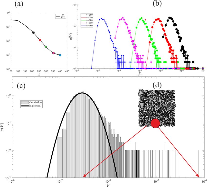
recorded in the previous computations. In Fig. 6 we show the critical curve acrit (r) on the [r, a] parameter plane, separat-
mass distribution of a system at r = 0.6 with N = 2000 par- ing systems where outliers may coexist with the population
ticles. The bulk of the histograms can be approximated well from systems where they may not. While we computed the
with a lognormal distribution. However, there are 12 particles acrit (r) critical curve for the case of infinitely large popula-
with somewhat larger volume than predicted by the lognor- tions (the N → ∞ limit), we stress the fact that the illustrated
mal distribution and one approximately 150 times the me- phenomenon is inherently discrete and does not arise in the
dian volume (5.3 times the radius). Thus inside the focusing continuum model. We may explain this curious phenomenon
regime we may observe a situation where we have a well- in the following manner. Assume that we start from a narrow
defined narrow distribution which describes the bulk of the distribution. Then random fluctuations in the discrete system
particles, but a few might escape from this process and may may create particles with large relative mass (i.e., a large pa-
be left behind, at larger mass. This effect is persistent and it rameter value a). If these fluctuations are sufficiently large
was observed also for the parameter value of r ' 0.7. to create particles above the critical curve acrit (r), then these
In order to estimate the robustness of this scenario we use outliers will be sustained; otherwise their mass will again ap-
a simple approximation by assuming that all but one particle proach the average mass of the majority. The critical curve in
have volume X and one single, exceptional particle, called Fig. 7 shows that in the vicinity of the critical value r = 0.5
https://doi.org/10.5194/esurf-9-235-2021 Earth Surf. Dynam., 9, 235–251, 2021244 A. A. Sipos et al.: Particle size dynamics in abrading pebble populations
Figure 6. Simulation of a finite sample with N = 2000 particles. Inset (a) shows the evolution of the mean volume normalized by the
maximal volume. Inset (b) depicts the evolution of the distribution; the corresponding points in (a) are denoted by the same color. The green
curve (t = 300) is the one shown in detail in panel (c); it depicts the particle volume histogram after 300 collisions per particle. The gray
boxes show the logarithmically binned histogram; the black line is a lognormal fit to the data. Observe the existence of outliers on the right.
Inset (d) is a visual illustration of the entire population: all particles are placed randomly into a 2D container. Smaller particles were placed
first and the white content (gray scale) is proportional to the linear size of the particle. One small particle close to the mean and one large
particle (outlier) are marked with red and their position is indicated in the distribution.
almost any such fluctuation will be sustained and outliers are 4 Conclusions
likely to survive. However, as the parameter r increases, it
becomes increasingly less likely to see sustained outliers. In this paper we presented the first statistical model for the
Another observation is that as the likelihood for the exis- collective mass evolution of pebble populations under colli-
tence of outliers decreases, their expected relative size in- sional abrasion. While our model is certainly not unique, it is
creases, which matches the common-sense observation that compatible with
the larger the outlier, the less frequently it may be observed.
a. existing geological observations,
We also note that the relationship between the collection of
small particles and the large particle is essentially asymmet- b. existing geometrical theory of individual and binary
rical. While the evolution of the latter is strongly influenced abrasion of pebbles,
by both the factor a and the control parameter r, the evolu-
tion of the density function for the small particles is solely c. existing theory for individual mass evolution of pebbles
controlled by the latter. In other words, adding one (or a few) (Sternberg’s law), and
very large particles to a collection of many small particles
d. exiting statistical theory of coagulation and fragmenta-
will not alter the fate of the latter, as long as the collisions
tion.
between a pair of particles are based on a uniform choice.
Earth Surf. Dynam., 9, 235–251, 2021 https://doi.org/10.5194/esurf-9-235-2021A. A. Sipos et al.: Particle size dynamics in abrading pebble populations 245
We investigated our model on two levels: (i) as a contin-
uum model by regarding the evolution of the Fokker–Planck
equation and (ii) as a discrete model by running discrete
event-based simulations. In the case of the continuum model
we derived our results analytically and also from numerical
simulation of the Fokker–Planck equation, while in the dis-
crete model we relied on numerical computations. With re-
gard to the existence of the critical parameter r = 0.5 and
the existence of the focusing and dispersing regimes, the two
approaches yielded quantitatively matching results.
Among many small pebbles, large boulders are often vis-
ible in mountain ranges or rivers. While this phenomenon is
commonly attributed to transport, our model suggests that
under some conditions, here again transport and abrasion
may act in unison: we identified a curios phenomenon not
present in the continuum model but present in the discrete
Figure 7. Critical curve acrit (r) on the [r, a] parameter plane. Sys- model (even in the N → ∞ limit). If the parameter r was in
tems with parameters (r, a) associated with points above the curve the focusing r > 0.5 range but not very far from the critical
permit the coexistence of outliers, while the systems associated with
value r = 0.5, the bulk of the distribution narrowed (in ac-
points below the critical curve do not permit the coexistence of out-
cordance with our analytical predictions); however, we could
liers. The solid line belongs to the N → ∞ limit, the dotted line
represents N = 20, and the dashed line N = 100 particles. also observe a few particles with substantially larger mass
(outliers), escaping the bulk of the distribution. We char-
acterized the mass ratio of outliers versus the mean of the
In the spirit of standard statistical theory for collective evo- bulk distribution by the parameter a, and we derived a crit-
lution, our model is based on two components: (i) the bi- ical curve acrit (r) separating systems where outliers may be
nary collision kernel and, based on that, (ii) the governing observed from those where this may not happen. Our result
equation for the evolution of probability density functions predicts that larger outliers are less likely to be observable.
for mass distribution. Regarding (i) we used the model from While our paper only dealt with size distributions, there
Domokos and Gibbons (2018), which incorporates the ex- exist also related observations on shape: sharp peaks in
isting theory for individual and binary abrasion; regarding distributions of axis ratios (also referred to as equilibrium
(ii) we used the Fokker–Planck equation, which is broadly shapes) are mentioned in Bluck (1967), Dobkins and Folk
used in the theory of coagulation in fragmentation. (1970), Landon (1930), Orford (1975), Williams and Cald-
Our collision kernel includes the single scalar parameter r well (1988), Ashcroft (1990), Lorang and Komar (1990),
which can be associated with the energy level of the collec- Yazawa (1990), and Wald (1990). In Domokos and Gibbons
tive collisional evolution process. We found that r = 0.5 is (2012) a plausible argument was presented that equilibrium
critical, separating two regimes with fundamentally differ- shapes may emerge on shingle beaches as the result of the
ent behavior: for r > 0.5 (low-energy regime) we found fo- interaction of abrasion and transport. We hope that the exten-
cusing behavior with decreasing relative variance R(t), and sion of the statistical theory presented in this paper may be
for r < 0.5 (high-energy regime) we found dispersing be- capable of verifying these observations.
havior with increasing relative variance R(t). In geological
terms, this result suggests that in low-energy environments
collisional abrasion acts on mass distributions in unison with
size-selective transport, while in high-energy environments
the opposite happens and the two processes counteract each
other. In accordance with prevailing geological observations
and Sternberg’s law, our models predicts exponential decay
of particle mass in both energy regimes.
https://doi.org/10.5194/esurf-9-235-2021 Earth Surf. Dynam., 9, 235–251, 2021246 A. A. Sipos et al.: Particle size dynamics in abrading pebble populations
Appendix A: Testing the model for heterogeneous will use m1 for the limestone and m2 for the granite. The joint
pebble populations evolution of such a heterogeneous population is described by
M 2 = 4 binary material constants: c11 , c12 , c21 , and c22 . At-
In the context of the binary evolution model (Eqs. 1–2) we tal and Lavé (2009) were primarily interested in the abrasion
introduced the binary abrasion parameters c12 and c21 and rates for limestone and they produced the Ed (D) plots for
for simplicity (since we only aimed to treat homogeneous these particles. In this experiment we may assume that the
populations) we used the same notation in the collision ker- abrasion of the limestone pebbles was exclusively due to col-
nel (Eqs. 3–4). Here we refine this concept in the statistical lisions with the granitic gravel (i.e., we disregard limestone–
setting for heterogeneous populations where we regard the limestone collisions). Thus the only relevant collisions are
collective evolution of N particles with M ≤ N different ma- between limestone and granite, and for the mass loss X(t)
terials mi , (i = 1, 2, . . . M). (The binary case corresponds to of the limestone we will use Eq. (3) with X and Y denoting
N = 2; if the two pebbles are made from different material, the volumes of the colliding limestone and granitic particles,
then we have M = 2, and for pebbles with identical materi- respectively, and c12 denoting the binary abrasion parame-
als we have M = 1. In the latter case in (Eqs. 1–2) we have ter associated with limestone being abraded by granite (not
c12 = c21 = c.) reported, but we may assume c21
c12 ). If we replace the
In the statistical setting the binary abrasion parameters volume of the granitic particles by their average, the abrasion
can be organized into an M × M matrix M with entries rate as function of its diameter can be calculated numerically.
cij , (i, j = 1, 2, . . . M). The binary parameter cij is defined Note that the abrasion rate Ed in our notation reads
as the constant coefficient in the collision kernel (Eqs. 3–
Xt
4) associated with the abrasion rate of particles with mate- Ed = − . (A1)
rial mi , bombarded by particles with material mj . Needless X
to say, the matrix M is not symmetrical; in general we have We fitted Eq. (3) to the dataset provided in Attal and Lavé
cij 6 = cj i . In particular, if material mi is much harder than (2009). We minimized the mean square error (with respect
material mj , then we expect cij
cj i . to the results in Attal and Lavé, 2009) for the parameters r
Based on the above considerations, the statistical model and c12 and obtained r = 0.19 and c12 = 0.28. Our fitted
is controlled by the M × M = M 2 binary abrasion parame- curves are illustrated in Fig. A1 showing fair agreement be-
ters and the single environmental parameter r. Testing this tween the data and the fitted model. The value of the environ-
model can be done along the strategies outlined in Sect. 1.4 mental parameter is in the range where we expect dispers-
for homogeneous populations; however, more detail has to ing behavior, as we discussed in Appendix D, which is in
be observed. accordance with the target of the original experiment which
simulated abrasion in fluvial environments. We note that the
a. One may test the model at the input level, by fitting the same parameter pair r = 0.19 and c12 = 0.28 is valid for both
kernel (Eqs. 3–4) to laboratory tests for pair-wise se- limestone experiments (i.e., these parameters do not depend
lected materials mi , mj . In such a test the abrasion rate on the size of the particle). Our fit appears to be consistent in
of particles of material mi under abrasion from parti- this respect.
cles of material mj is plotted as a function of particle
size of the abraded particle (with material mi ). Such ex- Appendix B: Some properties of the kernels in
periments can be used to determine the binary abrasion Sect. 2.3
parameters cij for a given heterogeneous population. If
the laboratory test imitates the environment of the natu- B1 Summation kernel
ral process, the environmental parameter r may also be
obtained in this manner. We will show such an example Differential equations governing the time evolution of the
below. first and second moments can be readily obtained; hence the
mean E + (t) and variance W + (t) follow the following initial
b. One may test the model at the output level by measuring value problems (IVPs):
the time evolution of full mass distributions and fitting
the M 2 material parameters cij and the environmental Et+ (t) = −2E + (t) with E + (0) = E0 , (B1)
parameter r to this dataset. Wt+ (t) = −2W + (t) +
with W (0) = W0 . (B2)
Next we show an example for testing the model at the in- It follows that both the expectation and the variance exhibit
put level by using the data obtained in Attal and Lavé (2009). exponential decay, namely E + (t) = E0 e−2t and W + (t) =
Here the authors report on flume experiments where they W0 e−2t . It is straightforward to show that the relative vari-
measured the abrasion rate Ed of individual limestone grav- ance R + (t) increases exponentially:
els with a diameter between D = 9 and D = 39 mm mixed in W + (t) W0
approximately 400 g of 10–18 and 18–28 mm granitic gravel. R + (t) := + 2
= 2 e2t = R0 e2t . (B3)
E (t) E0
In our terminology, we have M = 2 (two materials) and we
Earth Surf. Dynam., 9, 235–251, 2021 https://doi.org/10.5194/esurf-9-235-2021A. A. Sipos et al.: Particle size dynamics in abrading pebble populations 247
Using the master equation, the following Cauchy problems
are found that define the evolution of the mean and the vari-
ance:
1
Etc,T (t) = − E c,T (t) with E c,T (0) = E0 , (C2)
2
1
Wtc,T (t) = − + r W c,T (t) with W c,T (0) = W0 . (C3)
2
Solution of these ordinary differential equations (ODEs)
yields the evolution of the relative variance as
W c,T (t)
c,T W0 1
2 −r t
R (t) := c,T 2 = 2 e . (C4)
E (t) E0
Figure A1. Abrasion rate Ed predicted by the compound kernel
C2 A population of identical particles preserved
(Eq. 3) fitted to experimental data in Attal and Lavé (2009). Fig- Here we show that a population of identical particles, charac-
ure 9a by Attal and Lavé (2009) superposed with our model fits F1 terized by a Dirac-delta function as input PDF is preserved in
and F2 . Mass estimated from diameter. Least squares optimization
the model with the compound kernel regardless of the value
yields r = 0.19 and c12 = 0.28.
of parameter r. Without loss of generality, we investigate the
evolution from the f0 = δ(1) initial condition, where δ(x) de-
B2 Product kernel notes the Dirac-delta function at x. Obviously, E0 = 1 and
W0 = 0. We show that now f (t, x) = δ(c(t)) holds for any
In the case of the product kernel the IVPs describing the evo- t > 0. Let us assume that at some t ∗ ≥ 0, the distribution is
lution of the mean E ∗ (t) and variance W ∗ (t), respectively, f (t ∗ ∗) = 0. Observe that
read
Z∞
f t ∗ , y ψ c (x, y)dy = ψ c x, c t ∗ .
2
Et∗ (t) = − E ∗ (t) with E ∗ (0) = E0 , (B4) (C5)
Wt∗ (t) = −2W ∗ (t)E ∗ (t) with W ∗ (0) = W0 . (B5) 0
The time derivative of the mean can be computed via
Here the decay of the mean and the variance are polynomial
Z∞
as we find
Etc ∗
= ft t ∗ , x xdx
t
1
E ∗ (t) = and 0
t + E10 Z∞
1
= − f t ∗ , x ψ c x, c t ∗ dx = − c t ∗ , (C6)
W0 2 1 2
W ∗ (t) = 2 , (B6)
E0
0
t + E10
where we used Eq. (7), applied integration by parts, and em-
ployed Eq. (C5). Similarly, the evolution of the variance is
which result in a steady relative variance R ∗ (t), determined
found to follow
by the initial distribution f0 . Specifically
Z∞
W ∗ (t) Wt t = ft t ∗ , x x 2 dx − 2Etc t ∗ E c t ∗
c ∗
W0
R ∗ (t) := = 2 = R0 . (B7)
E ∗ (t)2 E0 0
Z∞
2
= −2 f t ∗ , x ψ c x, c t ∗ xdx + c t ∗
Appendix C: Approximate investigation of the
compound kernel 0
2 2
C1 Truncated compound kernel = −c t ∗ + c t∗ = 0. (C7)
The truncated compound kernel is obtained from the com- This shows that the variance of the distribution is constant,
pound kernel as the truncated Taylor polynomial computed and it started at W0 = 0; i.e., it vanishes entirely in its the
at y = x with an (O(y − x)2 : evolution. In other words, we have a Dirac-delta (degenerate)
distribution at any t ≥ 0. Employing Eq. (C6) we find that the
location c(t) follows the initial value problem ct (t) = − 12 c(t)
x 1 r
ψ c,T (x, y) := + − (y − x) + O (y − x)2 . (C1) with c(0) = 1; hence c(t) = exp(− 2t ).
2 4 2
https://doi.org/10.5194/esurf-9-235-2021 Earth Surf. Dynam., 9, 235–251, 2021You can also read