Online Learning with Radial Basis Function Networks
←
→
Page content transcription
If your browser does not render page correctly, please read the page content below
Financial Computing Group, UCL (2021)

                                               Online Learning with Radial Basis Function Networks

                                         Gabriel Borrageiro                                                gabriel.borrageiro.20@ucl.ac.uk
                                         Department of Computer Science
                                         University College London
                                         Gower Street, London, WC1E 6BT, UK
                                         Nick Firoozye                                                                   n.firoozye@ucl.ac.uk
                                         Department of Computer Science
                                         University College London
arXiv:2103.08414v2 [cs.CE] 23 Jun 2021

                                         Gower Street, London, WC1E 6BT, UK
                                         Paolo Barucca                                                                    p.barucca@ucl.ac.uk
                                         Department of Computer Science
                                         University College London
                                         Gower Street, London, WC1E 6BT, UK

                                                                                         Abstract
                                              We investigate the benefits of feature selection, nonlinear modelling and online learning
                                              when forecasting in financial time series. We consider the sequential and continual learning
                                              sub-genres of online learning. The experiments we conduct show that there is a benefit to
                                              online transfer learning, in the form of radial basis function networks, beyond the sequen-
                                              tial updating of recursive least-squares models. We show that the radial basis function
                                              networks, which make use of clustering algorithms to construct a kernel Gram matrix, are
                                              more beneficial than treating each training vector as separate basis functions, as occurs
                                              with kernel Ridge regression. We demonstrate quantitative procedures to determine the
                                              very structure of the radial basis function networks. Finally, we conduct experiments on
                                              the log returns of financial time series and show that the online learning models, partic-
                                              ularly the radial basis function networks, are able to outperform a random walk baseline,
                                              whereas the offline learning models struggle to do so.
                                              Keywords: online learning, transfer learning, radial basis function networks, financial
                                              time series, multi-step forecasting

                                         1. Introduction
                                              Financial time series are characterised by high serial autocorrelation and nonstationarity.
                                              The classic paper on the theory of option pricing by Black and Scholes (1973), assumes that
                                              stock prices follow a geometric Brownian motion through time, which produces a log-normal
                                              distribution of price returns. Merton (1976) modelled the dynamics of financial assets as a
                                              jump-diffusion process, which is now commonly used in financial econometrics. The jump-
                                              diffusion process implies that financial time series should observe small changes over time,
                                              so-called continuous changes, as well as occasional jumps. One approach for coping with
                                              nonstationarity, is to continuously learn online. Online learning can be classified into three
                                              broad areas: sequential updating, states of nature or transitional learning, and continual
                                              learning.
                                                   Sequential learning in time is a self-explanatory concept and has a rich history. The
                                              Kalman filter (Kalman, 1960) is a state space model which was originally designed for
                                              tracking objects in time, such as airplanes or missiles, from noisy measurements, such

                                         ©2021 Gabriel Borrageiro, Nick Firoozye and Paolo Barucca.
                                         License: CC-BY 4.0, see https://creativecommons.org/licenses/by/4.0/. Attribution requirements are provided
                                         at http://jmlr.org/papers/v/.html.
Borrageiro, Firoozye and Barucca

as radar. Several approaches exist for sequential learning in nonstationary data. These
include discounted least squares (Abraham and Ledolter, 1983) and exponentially weighted
recursive least squares (Liu et al., 2010). Barber et al. (2011) consider Bayesian approaches
to time series modelling which are amenable to sequential learning.
     Transitional learning includes reinforcement learning, which allows agents to inter-
act with their environment, mapping situations to actions so as to maximise a numerical
award. Well known online reinforcement learning algorithms include q-learning (Watkins,
1989) and sarsa (Rummery and Niranjan, 1994). The classical k-armed bandit problem,
where one is faced with a choice amongst k possible options, is formulated as an online
learning problem. After each choice, a reward is assigned. The interplay between hedonis-
tic exploitation and potentially costly exploration, leads to a number of algorithms such
as -greedy, stochastic gradient ascent and upper confidence bound bandits (Sutton and
Barto, 2018).
     Continual learning is an area of study that asks how artificial systems might learn
sequentially, as biological systems do, from a continuous stream of correlated data (Hadsell
et al., 2020).They include gradient based methods (Kaplanis et al. 2018, Kirkpatrick et al.
2017), meta learning (Wang et al., 2017) and transfer learning (Yang et al., 2020). The
goal of transfer learning is broadly to transfer knowledge from one model (the source) to
another (the target). Sub-paradigms of transfer learning include inductive, where labelled
data is available in the target domain, and transductive, where labelled data is available
only in the source domain. Koshiyama et al. (2020) applies transfer learning to systematic
trading strategy development, with goals of minimising backtest overfitting and generating
higher risk adjusted returns.
     In our paper, we aim to assess the benefits of predictive modelling, feature selection,
online learning and nonlinear modelling. We limit the scope of our experimentation to
financial time series, which at times exhibit high autocorrelation, nonstationarity and non-
linearity. This behaviour might be classified as concept drift (Iwashita and Papa, 2019).
On its own, the sequential learning approach to online learning might be suboptimal to
an approach that includes other forms of online learning such as transfer learning. The
marquis model of this paper, an online learning radial basis function network, employs two
models. The unsupervised learning step, which learns the hidden processing units of the
network, is capable of time series pattern recognition. The supervised learning step, which
maps these hidden processing units to the output, employs sequential learning. The model
thus straddles the continual learning and sequential learning domains. For this reason, we
explore its benefits within forecasting financial time series.
     Through experimentation, we wish to ask several research questions and test several
hypotheses. A first question would be, should predictive modelling consistently outperform
model free approaches as it pertains to forecast accuracy? A second research question is,
is there a benefit to doing feature selection? Related to this question, should we look at
exogenous features? The likes of Chatfield (2019) caution against the indiscriminate use of
exogenous features. The reasons he gives include the introduction of serial autocorrelation
in the regression residuals, leading to spurious regressions (Granger and Newbold, 1974) and
the belief that exogenous features should provide clear contextual reasons as to why they
should be included, rather than considering optimisation criteria alone, such as squared-
error loss minimisation. A further research question is, even after making time series
stationary, should online learning outperform offline learning? The hypothesis of a jump-
diffusion process implies that even if returns are constructed, and tests such as the Dickey
and Fuller (1979) imply data stationarity, occasional jumps might still occur, which render
the offline learning models less useful. We expect a priori for the relationship between a set
of predictors and a target to be changing over time, thus requiring some form of sequential
learning. To test this hypothesis, we create some online learning models and measure their

                                              2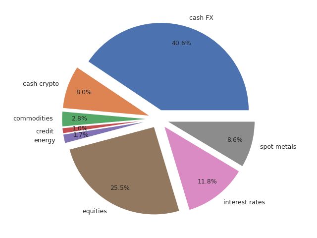
Online Learning with Radial Basis Function Networks

   performance against some offline learning models. All models are then baselined against a
   random walk model.

1.1 Our Contribution
   Our paper contributes to the research of continual learning in financial time series. This is
   important as our experiment shows that continual learning provides a benefit with multi-
   step forecasting, above and beyond sequential learning. If we compare the local learning
   of the radial basis function network with the global learning technique of the feed-forward
   neural network, the latter suffers from catastrophic forgetting. The radial basis function
   network that we formulate, is naturally designed to measure the similarity between test
   samples and continuously updated prototypes that capture the characteristics of the feature
   space. As such, the model is somewhat robust in mitigating catastrophic forgetting.
        Although closely related to kernel Ridge regression, our experiment results show that
   the radial basis function networks, which make use of clustering algorithms, and therefore
   have condensed hidden processing units, are more beneficial than treating each training
   vector as separate basis functions. Indeed, considering the regret bounds of section 4, then
   the regret with respect to the expert with forward looking bias, scales with the number of
   experts. Thus, care should be taken as to how those experts are formulated and chosen.
   Furthermore, if one makes use of the Nyström approximation to the kernel Gram matrix,
   as shown in algorithm 2, random sub-sampling of the feature space is of less benefit than
   employing clustering or pseudo-clustering algorithms to construct a kernel Gram matrix
   for use in modelling non-stationary data, such as financial time series.
        In terms of selecting the structure of the radial basis function network itself, namely se-
   lection of the hidden processing units, we have demonstrated quantitative procedures to do
   so, which are less expensive than procedures based on cross-validation or generalised cross-
   validation alone. For the radial basis function network that makes use of kmeans++, we
   consider several possible cluster structures and select the one that maximises the silhouette
   score, see section 3.2.1. For the radial basis function network that makes use of Gaus-
   sian mixture models, we use the meta-algorithm and modified expectation-maximisation
   procedure outlined by Figueiredo and Jain (2002) and discussed in section 3.2.2, to se-
   lect mixtures that provide both mixture selection and model estimation. In addition, the
   specific formulation annihilates mixtures that are not supported by the data.
        Finally, we show a feature selection meta-algorithm that combines two algorithms,
   namely forward stepwise selection and variance inflation factor minimisation. The former
   is used to select features that have explanatory power with respect to the response, even
   in a high dimensional feature space setting, and the latter is used to prune any correlated
   features back, which are likely to result in greater prediction variance.

2. Preliminaries
   We begin with a discussion of the baseline model and the preliminary models that we use
   in our experimentation. Also discussed is a feature selection meta-algorithm that we make
   use of.

2.1 The Random Walk Model
   As described in Harvey (1993), the simplest non-stationary process is the random walk
   model
                                           yt = yt−1 + t .

                                                  3
Borrageiro, Firoozye and Barucca
This is the model we use as a baseline in the experiments we conduct. The first differences
of this model, yt − yt−1 , are stationary, which leads to a general class of models known as
autoregressive integrated moving average (arima). Repeatedly substituting for past values
gives
t−1
X
yt = y0 + t−i .
i=1
The expectation of the random walk model is
E[yt ] = y0 ,
indicating a constant mean over time. The variance of a random walk process
V ar[yt ] = tσ 2 ,
and covariance
Cov[yt , yt−τ ] = |t − τ ]σ 2 ,
is however, non-stationary. It is common within econometrics to take log first differences,
as this has a variance stabilising effect. Let us denote the h-step ahead log return as
h
X
yt+h = log(Yt+h /Yt ) = log(Yi /Yi−1 ),
i=t+1
where, in the context of financial time series for example, Yt would typically represent a
quoted price at time t. When forecasting using the random walk model in log returns space,
the mean square prediction error (mspe) for the h0 th forecast horizon becomes
t−h t−h
1 X 1 X 2
mspeh = (yi+h − ŷ0 )2 = y .
t − h i=1 t − h i=1 i+h
A large amount of academic literature shows that it is difficult to beat the random walk
model when forecasting returns of financial time series. For example, Meese and Rogoff
(1983) show that the monetary, econometric model is unable to outperform a random
walk model when forecasting currency exchange rates, which implies that exchange rates
behave in a purely random and unpredictable manner. This phenomenon is known as
the Meese–Rogoff puzzle. Engel (1994) worked further on this puzzle. He fits a Markov-
switching model to 18 exchange rates at sampled quarterly frequencies, and finds that the
model fits well in-sample for many exchange rates. However, by the mean square prediction
error criterion, the Markov model does not generate superior forecasts to a random walk
for the forward exchange rate. He finds some evidence to support that the forecasts of the
Markov-switching model are superior at predicting the direction of change of the exchange
rate. More recently, Ince et al. (2019) provide exchange rate forecasting by combining
vector autoregression models with multi-layer feed-forward neural networks. Their models
are able to outperform the random walk baseline on currency returns sampled monthly
and forecasted one step ahead. They conclude that employing alternative artificial neural
network structures such as radial basis function networks and recurrent neural networks
remain as relevant future research topics.
2.2 The Autoregressive(1) Model
As Harvey (1993) discusses, the autoregressive model of order 1
yt = φ1 yt−1 + t , t = 1, ..., T,
4Online Learning with Radial Basis Function Networks
is closely related to the random walk model. We denote this model as ar(1). Substituting
repeatedly for lagged values of yt gives
t−1
X
yt = φi t−i + φt y0 .
i=1
The expectation of the ar(1) model is
t−1
X
E[yt ] = E φi t−i + E[φt y0 ] = φt y0 .
i=1
For |θ| ≥ 1, the mean value of the process depends on the starting value, y0 . For |θ| < 1,
the impact of the starting value is negligible asymptotically. The variance of the ar(1)
process is
t−1
X ∞
X
γ[0] = E φi t−i = σ 2 φ2i = σ 2 /(1 − φ2 ).
i=1 i=1
2.3 Feature Selection
Linear regression is a model of the form
p(y|x, θ) = N (y|wT x, σ 2 ),
where y is the response, x is the vector of independent variables, and the parameter set θ =
[w, σ 2 ], must be estimated. The assumption is that the conditional probability p(y|x, θ),
is normally distributed. How should we select the predictor set x, where x ⊂ X ? In
the spirit of Occam’s razor, we seek a subset of minimally correlated predictors, with
maximal explanatory power. There are various feature selection algorithms, which Hastie
et al. (2009) discuss in detail. Here, we show a feature selection meta-algorithm that
combines two algorithms, namely forward stepwise selection and variance inflation factor
minimisation. The former is used to select features that have explanatory power with
respect to the response, even in a high dimensional feature space setting, and the latter
is used to prune any correlated features back. Correlated features are likely to result in
greater prediction variance. In the algorithm that follows, κ is the maximum variance
5Borrageiro, Firoozye and Barucca
inflation factor that is permitted, X is the n × d predictor matrix, and y is the n × 1 target
vector.
Algorithm 1: forward stepwise selection with variance inflation factors
Require: κ
Initialise: S = [1, 2, ..., d], r = v = [0, ..., 0] ∈ Rd
Input: X, y
Output: S ∈ Rp , 0 < p ≤ d
1 for j ← 1 P to d do
n
2 ȳ = n1 i=1 yi
1
Pn
3 x̄j = Pn i=1 Xij
n
(y −ȳ)(Xij −x̄j )
4 θj = Pn i
i=1
2
i=1 (Xij −x̄j )
// rj is the r-squared of a regression of y onto Xj .
Pn 2
2 i=1 (yi −θj Xij )
5 rj = Ry|X =1− P n 2
j i=1 (yi −ȳ)
2
// RX j |X−j
denotes the r-squared of a regression of Xj onto the
// remaining predictors, excluding the j 0 th one.
6 vj = 1−R21
Xj |X−j
7 end
8 Sort r from smallest to largest and use its sort index to sort S.
9 while ∀v >= κ do
10 for j ← 1 to m do
11 if vj >= κ then
12 remove Sj
13 recompute v
14 end
15 end
16 end
2.4 Kernel Ridge Regression
The Ridge regression model of Hoerl (1962) minimises the cost function
n d
1X 1X T
Jθ = (yi − θ T xi )2 + λθ θ j . (1)
2 i=1 2 j=1 j
The regression parameters can be estimated sequentially in an online manner
t
X t
−1 X
θ̂ t = xt xTt + λId x t yt . (2)
i=1 i=1
Ridge regression is amenable to being kernelised. Following Murphy (2012), let us define a
0 0
kernel function to be a real-valued function of two arguments, K(x, x ) ∈ R, for x, x ∈ X , X
being some abstract space. Typically the kernel function is symmetric and non-negative.
A suitable kernel function for measuring similarity between vectors, is the radial basis
function
0 1 0 T −1 0
K(x, x ) = exp − (x − x ) Σ (x − x ) , (3)
2
The scalar variance version
k x − x0 k2
K(x, x0 ) = exp − , (4)
2σ 2
6Online Learning with Radial Basis Function Networks
is seemingly more popular, most likely as the full covariance matrix can show greater
prediction variance when used to generate features for a supervised learner. Let us the
define the kernel Gram matrix
K(x0 , x0 ) . . . K(x0 , xn )
K= ..
.
.
K(xn , x0 ) . . . K(xn , xn )
Equations 1 and 2 can be thought of as a primal optimisation problem. We are then able
to make use of the so-called kernel trick, which replaces all innner products of the form
x, x0 with kernel functions K(x, x0 ). In the dual optimisation problem, we define the dual
variables as
α = (K + λIn )−1 y,
which allows us to rewrite the primal variables as
n
X
θ = XT α = αi xi .
i=1
The test time predictive mean is thus
n
X n
X
ŷt = fˆ(xt ) = θ T xt = αi xTi xt = αi K(xi , xt ).
i=1 i=1
As described by Vovk (2013), kernel Ridge regression was first coined by Cristianini
and Shawe-Taylor (2000), and is a special case of support vector regression (Vapnik, 1998).
Vovk goes on to show that kernel Ridge regression has certain performance guarantees that
do not require any stochastic assumptions to be made. Specifically, he shows that for any
sequence of time steps, the model satisfies
n n
(yt − ŷt )2
X X
2 2
= min (yt − ŷt ) + λ k f kF ,
t=0
1 + λ1 K(xt , xt ) − λ1 kTt (Kt−1 + λIn )−1 kt f ∈F
t=0
where kt is the vector with components
K(x0 , xt )
kt = ..
.
.
K(xn , xt )
In addition, assuming |yt | ≤ ymax , and yˆt is similarly clipped |yˆt t | ≤ ymax , then the sum
of squared errors is bounded as:
n Xn
X 1
(yt − ŷt )2 ≤ min (yt − ŷt )2 + λ k f k2F + 4ymax
2
ln det In + Kt .
t=0
f ∈F
t=0
λ
A practical difficulty with kernel Ridge regression, is that model fitting scales as O(n3 ).
Williams and Seeger (2001) show that an approximation to the eigen-decomposition of the
Gram matrix can be computed by the Nyström method, which is used for the numerical
solution of eigen-problems. This is achieved by carrying out an eigen-decomposition on a
smaller system of size m < n, and then expanding the results back up to n dimensions.
The computational complexity of a predictor using this approximation is O(m2 n). On
experiments they conduct with a Gaussian process classifier, they demonstrate that the
7Borrageiro, Firoozye and Barucca
Nyström approximation to the kernel Gram matrix allows a very significant speed-up of
computation, without sacrificing accuracy. Pseudo-code for the algorithm is shown next.
Algorithm 2: the Nyström approximation to the kernel Gram matrix
Require: p, m, with p ≤ m < n
Input: X ∈ Rn×d
Output: Z ∈ Rm×p , typically with d < p
1 Construct the kernel Gram matrix K̃ ∈ Rm×m using random sampling.
2 Compute a singular value decomposition K̃ = ŨΛ̃ŨT , where Ũ is orthonormal, and Λ̃ is a
diagonal matrix of ranked eigenvalues, with λ̃0 ≥ λ̃1 ≥ ... ≥ 0.
3 Take the first p columns of Ũ and the first p eigenvalues of Λ̃ to form M̃ = Ũ:p Λ̃:p , with
M̃ ∈ Rm×p .
4 Reconstitute the kernelised predictor matrix Z = K̃M̃, and pass this to the supervised
learner of your choice.
3. The Radial Basis Function Network
The radial basis function network is a single layer network, where the hidden processing
units play the role of K, the kernel Gram matrix of kernel Ridge regression, see figure 1.
However, the number of hidden processing units k in the radial basis function network,
is usually k
n. The hidden processing units are commonly estimated via a clustering
algorithm, rather than randomly selecting a subset of n training vectors as per the Nyström
approximation to the kernel Gram matrix. Following Bishop (1995), the k th output of the
radial basis function network is defined as:
m
X
yk (x) = θkj φj (x) + θk0 ,
j=1
where θkj is the weight going from the j th basis function (hidden processing unit) to the k th
output. In the case of a real-valued output, k = 1. The bias θk0 can be absorbed into the
summation by defining an extra basis function φ0 with an activation set to 1. Nonlinearity
is introduced into the network via the Gaussian basis function
!
k x − µj k22
φj (x) = exp − ,
2σj2
where x is a d-dimensional input vector, µj is the centre of the basis function φj (.) and σj2
is its width. Let Φ denote the set of hidden processing units with functions φj (x) that have
been aggregated together. Bishop shows that the width σj2 can be replaced by a covariance
matrix Σj , leading to basis functions of the form
1 T −1
φj (x) = exp − (x − µj ) Σj (x − µj ) . (5)
2
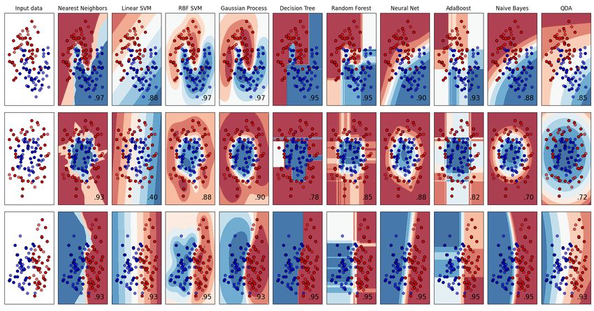
Figure 2 demonstrates a comparison of a several classifiers on synthetic datasets. As
Bishop (1995) discusses, a multi-layer perceptron separates classes using hidden units which
form hyperplanes in the input space. Alternatively, separation of class distributions can be
modelled by local radial basis kernel functions. The activations of the radial basis functions
can be interpreted as the posterior probabilities of the presence of corresponding features
in the input space, and the weights can be interpreted as the posterior probabilities of class
membership, given the presence of the features.
8Online Learning with Radial Basis Function Networks
Figure 1: architecture of the radial basis function network
Figure 2: comparison of a several scikit-learn classifiers on synthetic datasets
3.1 Literature Review
Girosi and Poggio (1990) show that radial basis function networks have a ”best approxima-
tion” property, that is, in the set of approximating functions corresponding to all possible
choices of parameters, there is one function which has minimum approximating error. Sem-
inal papers on radial basis function networks include those of Broomhead and Lowe (1988)
and Moody and Darken (1989). Moody and Darken’s approach to network training, is
extremely fast. It involves an unsupervised learning step, using a clustering algorithm
9Borrageiro, Firoozye and Barucca
such as k-means (Lloyd, 1982) to learn the hidden processing unit means µ, and a su-
pervised learning model such as Ridge regression which maps the hidden processing units
Φ, to the output, y. They make use of a scalar variance term as in equation 4, rather
than the full covariance as per equation 3. This method involves computing a ”global first
nearest-neighbor” heuristic, which uses a uniform average width σ = ∆xαβ for all hid-
den processing units, where ∆xαβ is the Euclidean distance in input space between unit α
and its nearest-neighbor β, and indicates a global average over such pairs. The fitting
complexity for Moody and Darken’s algorithm is O(knr) for the kmeans part, where k is
the number of clusters and r is the number of fitting iterations, and O(n2 p + p3 ) for the
linear regression part.
Billings et al. (1996) consider a modified method of Moody and Darken’s to network
training. They consider a large input space in X and a large hidden network space in µ,
relying on orthogonal least squares (Markovsky and Van Huffel, 2007) and forward stepwise
selection to select the hidden processing units. Finally, they employ recursive least squares
(Harvey, 1993) to map the hidden processing units to the response on an online basis. They
make the link between the nonlinear autoregressive moving average model with exogenous
inputs (Chen and Billings, 1989) and the radial basis function network, demonstrating an
application to multiple input multiple output modelling (Bontempi, 2008) in simulated
dynamic time series. A downside of their approach is that there is likely to be a lot of
redundancy in the input space, and in practical real-time application, it may be wasteful
to compute many predictors, only to potentially throw them away during network training.
Kanazawa (2020) applies an offline radial basis function network based on Moody and
Darken’s technique, to macroeconomic data. He finds that the estimated impulse responses
from the model, suggest that the response of macroeconomic variables to a positive supply
shock, is substantially time variant. He also finds that the model outperforms benchmarks
based on the vector autoregression and threshold-var estimators, but only with longer
term forecasts, 10 steps ahead or more. Overall, he finds that the model can uncover the
structure of data generated from the nonlinear new Keynesian model, even from a small
sample of simulated data. We can draw parallels between this outcome and the concept of
few shot learning (Wang et al., 2017), where the learner can rapidly generalize to new tasks
containing only a few samples of supervised information. He employs the renormalised
radial basis function approach of Hastie et al. (2009)
φc (x)
hc (x) = Pk ,
j=1 φj (x)
which aims to fill any holes in regions of Rd where the kernels have no appreciable support.
Khosravi (2011) demonstrates an approach to radial basis function network training
which is similar to backpropogation for neural networks (Rumelhart et al., 1986), although
he sets some weights between the inputs and hidden layer, rather than the traditional
approach, which has weights from the hidden layer to the outputs. He calls this his weighted
rbfnet, and finds improved accuracy on the UCI letter classification dataset and the HODA
digit recognition dataset.
The radial basis function network relates to the relevance vector machine of Tipping
(1999). Originally, Tipping created this model as a sparse, Bayesian alternative to the sup-
port vector machine. The sparsity is induced by defining an automatic relevance determina-
tion Gaussian prior (MacKay 1994, Neal 1996) over the model weights. The model param-
eters are estimated via iterative reestimation of the individual weight priors α, through ex-
pectation maximisation (Dempster et al., 1977). Rasmussen and Quiñonero-candela (2005)
make the link between the relevance vector machine and the Gaussian process model, where
the former’s hyper-parameters are parameters of the latter’s covariance function. Being a
10Online Learning with Radial Basis Function Networks
local learning technique, Rasmussen and Quiñonero-candela highlight that whilst the rel-
evance vector machine provides full predictive distributions for test cases, the predictive
uncertainties have the unintuitive property that they get smaller the further you move away
from the training cases. They propose to augment the relevance vector machine by an ad-
ditional basis function centered at the test input, which adds extra flexibility at test time,
thus improving generalisation performance. Gaussian process regression has an O(n3 ) time
complexity and an O(n2 ) memory complexity, and is thus more computationally expensive
to fit than the radial basis function network formulated by Moody and Darken. Further-
more, Moody and Darken’s radial basis function network is in effect making use of transfer
learning: the knowledge of the clustering model is transferred to the supervised learner,
and the intrinsic nature of the feature space is learnt and made available to the upstream
model.
3.2 Clustering Algorithms
Assuming the Moody and Darken approach to radial basis function network formulation,
there are several clustering algorithms that are suitable for use in deriving the hidden
processing units. We discuss a few of these, which meet the following criteria:
1. The clustering algorithm can provide hidden processing unit means µ0 , ..., µk .
2. Covariance matrices Σ0 , ..., Σk and their inverses (precision matrices) can be estimated and
associated with each cluster mean.
3. The cluster means and covariances can be estimated online, sequentially.
4. The number of clusters, and in effect the network size of the radial basis function network,
can be estimated quantitatively, without a more expensive estimation procedure such as cross-
validation.
All the clustering algorithms discussed next, can have their means updated sequentially in a
manner similar to equation 6. The precision matrices, which are required in equation 5, can
be estimated in a manner similar to algorithm 4, or with exponential decay as in algorithm
3. All that is required is for the clustering algorithm or pseudo-clustering algorithm to
make an assignment to the c0 th cluster at test time.
3.2.1 Kmeans
In the classical kmeans algorithm, one selects k cluster centres a priori, and the training
data x ∈ Rd is assigned to the nearest cluster centre, with a goal of minimising the sum of
squared distances. Usually these k centres are initialised at random. Each training vector
is then assigned to the nearest center, and each center is recomputed as the mean of all
points assigned to it. These two steps of assignment and mean calculation, are repeated
until the process stabilises, or a maximum number of iterations is exceeded. The training
error is
k X
X n
Jk = δji k xi − µj k22 .
j=1 i=1
Here δji is 1 when the training exemplar xi belongs to the processing unit µj , and 0
otherwise. A further advantage of this approach is that it is amenable to online learning.
A partial or online update takes the form
∆µj = η(xi − µj ), (6)
11Borrageiro, Firoozye and Barucca
where η is a learning rate in [0, 1]. Denote the optimal, minimal training error as Jk∗ . Due
to ’unlucky’ random initialisation of the cluster means, the ratio JJk∗ is unbounded, even for
k
fixed n and k. Arthur and Vassilvitskii (2007) demonstrate a way of initializing k-means
by choosing random starting centers with very specific probabilities. They select a point
i as a centre with probability proportional to the overall potential. Let D(x) denote the
shortest distance from a data point x to the closest centre already chosen. The next centre,
0 2
denoted as µc = x0 , is then chosen with probability PnD(xD(x )
i)
2 . They are able to upper
i=1
bound the loss of their so-called kmeans++ algorithm as
E[Jk ] ≤ 8(ln k + 2)Jk∗ .
Having estimated the cluster means µj , we are able to extract the cluster covariances
k n
1 XX
Σj = δji (xi − µj )(xi − µj )T , (7)
nk − 1 j=1 i=1
Pk Pn
where nk = j=1 i=1 δji . How might we select the number of clusters k in a fast,
quantitative manner? The silhouette score of Rousseeuw (1987) provides one solution.
Denote as ai the average dissimilarity of datum i to all other objects clustered in A, ci the
average dissimilarity of i to all other objects clustered in C, and bi = min di .
C6=A
The silhouette score for the i0 th datum is
1 − ai /bi
if ai < bi
si = 0 if ai = bi ,
bi /ai − 1 if ai > bi
or equivalently
bi − a i
si = .
max(ai , bi )
Thus −1 ≤ si ≤ 1. Averaging the si over all samples allows us to select the number of
clusters k such that
k ∗ = max(s̄0 , ..., s̄J ). (8)
PJ
The approach has time complexity of j O(kj nr), where kj is the number of clusters
for the j 0 th clustering, n the number of training examples and r is the number of fitting
iterations.
3.2.2 Gaussian Mixture Models
Gaussian mixture models facilitate a probabilistic, parametric based approach to clustering,
where the data generating process is assumed to be a mixture of multivariate Normal
densities. Denote the probability density function of a k component mixture as
k
X k
X
p(x|θ) = πj p(x|θ j ) = πj N (x|µj , Σj ),
j=1 j=1
where
1 1
N (x|µ, Σ) = exp − (x − µ)T Σ|−1 (x − µ) , (9)
(2π)d/2 |Σ|1/2 2
12Online Learning with Radial Basis Function Networks
Pk
and the mixing weights satisfy 0 ≤ πj ≤ 1, j=1 πj = 1. The maximum likelihood
estimate
θ M L = arg max ln p(x|θ),
θ
and the Bayesian maximum a posteriori criterion
θ M AP = arg max ln p(x|θ) + ln p(θ),
θ
cannot be found analytically. The standard way of estimating θ M L or θ M AP is the
expectation-maximisation algorithm (Dempster et al., 1977). This iterative procedure is
based on the interpretation that x is incomplete data. The missing part for finite mixtures
is the set of labels Z = z0 , ..., zn which accompany the training data x0 , ..., xn , indicating
which component produced each training vector. Following Murphy (2012), let us define
the complete data log likelihood to be
n
X
`c (θ) = ln p(xi , zi |θ),
i=1
which cannot be computed, since zi is unknown. Thus, let us define an auxiliary function
Q(θ, θ t−1 ) = E[`c (θ)|x, θ t−1 ],
where t is the current time step. The expectation is taken with respect to the old parameters
θ t−1 and the observed data x. Denote as ric = p(zi = c|xi , θ t−1 ), the responsibility that
cluster c takes for datum i. The expectation step has the following form
πc p(xi |θ c,t−1 )
ric = Pk .
j=1 πj p(xi |θ j,t−1 )
The maximisation step optimises the auxiliary function Q with respect to θ
θ t = arg max Q(θ, θ t−1 ).
θ
The c0 th mixing weight is estimated as
n
1X rc
πc = ric = .
n i=1 n
The parameter set θ c = {µc , Σc } is then
Pn
i=1 ric xi
µc =
rc
Pn
i=1 ric (xi − µc )(xi − µc )T
Σc = .
rc
As discussed by Figueiredo and Jain (2002), expectation-maximisation is highly de-
pendent on initialisation. They highlight several strategies to ameliorate this problem,
such as multiple random starts, with final selection based on the highest maximum like-
lihood of the mixture, or kmeans based initialisation. However, in mixture models, the
distinction between model-class selection and model estimation is unclear. For example, a
3 component mixture in which one of the mixing probabilities is zero, is indistinguishable
for a 2 component mixture. They propose an unsupervised algorithm for learning a finite
13Borrageiro, Firoozye and Barucca
mixture model from multivariate data. Their approach is based on the philosophy of mini-
mum message length encoding (Wallace and Dowe, 1999), where one aims to build a short
code that facilitates a good data generation model. Their algorithm is capable of selecting
the number of components and unlike the standard expectation-maximization algorithm,
does not require careful initialization. The proposed method also avoids another drawback
of expectation-maximization for mixture fitting: the possibility of convergence toward a
singular estimate at the boundary of the parameter space. Denote the optimal mixture
parameter set
θ ∗ = arg min `F J (θ, x),
θ
where
k
nX nπk k n k(n + 1)
`F J (θ, x) = ln + ln + − ln p(x|θ).
2 j=1 12 2 12 2
This leads to a modified maximisation step
Pn n
max 0, i=1 ric − 2
πc =
Pk Pn n
j=1 max 0, r
i=1 ij − 2
f or c = 1, 2, ..., k.
The maximisation step is identical to expectation-maximisation, except that the c0 th pa-
rameter set θ c is only estimated when πc > 0, and θ c is discarded from θ ∗ when πc = 0.
A distinctive feature of the modified maximisation step is that it leads to component an-
nihilation. This prevents the algorithm from approaching the boundary of the parameter
space. In other words, if one of the mixtures is not supported by the data, it is annihilated.
3.2.3 Discriminant Analysis As A Pseudo-Clustering Algorithm
When we consider the four selection criteria stated at the start of section 3.2, quadratic
discriminant analysis, where we must estimate class-conditional means and covariances,
modelled by multivariate normal distributions, could be considered as a pseudo-clustering
algorithm. Instead of an unsupervised learning step to infer labels, we can create labels from
the regression responses, and derive the class-conditional parameter sets θ c = {µc , Σc }.
For financial time series, an obvious set of classes is {−1, 0, 1}, corresponding to the signed
mid to mid returns. There is a sound, scientific rationale for deriving class-conditional
covariates for such time series. It is well known amongst financial practitioners that down-
side volatility of returns behaves differently to up-side volatility, particularly for equities.
In the plot and tabular summary shown next, we display annualised volatility (standard
deviations) computed from 21 day sliding windows of daily mid to mid returns for the S&P
500 equity index. The data are extracted from Refinitiv. The volatilities are separated out
by negative and positive daily returns. We see that since the 1987 stock market crash, so-
called ’Black Monday’, annualised volatility is around 0.8 of a percent higher for downside
returns.
regime count mean std min q25 q50 q75 max ann vol
-1 11219 -0.78% 0.92% -20.47% -1.00% -0.51% -0.22% 0.00% 14.60%
1 12696 0.74% 0.86% 0.00% 0.23% 0.50% 0.95% 16.61% 13.72%
Table 1: .SPX annualised volatility by regime
14Online Learning with Radial Basis Function Networks
Figure 3: .SPX annualised volatility by regime
3.3 Regularisation Of Covariance Matrices And Their Inverses
A central issue for the algorithms discussed in sections 3.2.1, 3.2.2 and 3.2.3, is the es-
timation of covariance matrices, that are required by the radial basis function network.
As highlighted by Friedman (1989), equation 7 produces biased estimates of the eigen-
values; the largest ones are biased high and the smallest ones are biased toward values
that are too low. He goes on to say that the net effect of this biasing phenomenon on
discriminant analysis is to (sometimes dramatically) exaggerate the importance associated
with the low-variance subspace spanned by the eigenvectors corresponding to the smallest
sample eigenvalues. Aside from this, we need a way to reduce or mitigate completely, the
numerical issues that appear when estimating covariance matrices where n < d, the number
of predictors is larger than the number of observations. Friedman’s procedure to regularise
covariance matrices involves two steps. Let us define the pooled covariance estimate as
Σ, which is estimated from all the training data. In the first step, we shrink the class
conditional covariance toward the pooled estimate
Σc (λ) = (1 − λ)Σc + λΣ,
where 0 ≤ λ ≤ 1. In the second step, we shrink Σc (λ) toward a multiple of the identity
matrix
γ
Σc (λ, γ) = (1 − γ)Σc (λ) + trace[Σc (λ)]I,
d
with 0 ≤ γ ≤ 1. A standard way to estimate λ and γ is through cross-validation. Another
area in which stability can be gained, is to estimate the determinant of the covariance
15Borrageiro, Firoozye and Barucca
matrix of equation 9, via a spectral decomposition
k
X
T
Σc = ejc vjc vjc ,
j=1
where ejc is the j 0 th eigenvalue of Σc in decreasing value, and vjc is the corresponding
eigenvector. The stabilised determinant of the covariance matrix for the multivariate nor-
mal is then
k
X
|Σc | = max(0, ejc ).
j=1
3.4 Exponentially Weighted Recursive Least Squares
Once we have selected the hidden processing unit centres and covariances using any of the
algorithms in section 3.2, we must then map this new predictor space to the regression
target. A suitable supervised learning algorithm, is the recursive least squares estimator,
which is a special case of the Kalman filter (Harvey, 1993). In particular, we are interested
in the exponentially weighted formulation, see Liu et al. (2010), which facilitates adaptation
sequentially in time. The algorithm we show below, includes a variance stabilisation update,
which ameliorates the build-up of large values along the diagonal of the precision matrix P,
which may occur if the response y has low variance. See for example Gunnarsson (1996) for
a further discussion on the regularisation of recursive least squares. Similar regularisation
approaches suitable for online learning and nonstationary data are studied by Moroshko
et al. (2015).
Algorithm 3: exponentially weighted recursive least squares
Require: λ // the Ridge penalty
1 0
τ < 1 // an exponential forgetting factor
Initialise: θ = 0, P = Id /λ
Input: xt ∈ Rd×1 , yt
Output: ŷt
2 r = 1 + xTt Pt−1 xt /τ
3 k = Pt−1 xt /(rτ )
4 θ t = θ t−1 + k(yt − θ Tt−1 xt )
5 Pt = Pt−1 /τ − kkT r
6 Pt = Pt τ // variance stabilisation
7 ŷt = θ Tt xt
4. Ensemble Learning
We have shown that feature selection can be achieved through the meta-algorithm 1. In
addition, the hidden processing units of the radial basis function network, with centres and
covariances chosen by the clustering algorithms of section 3.2, can be thought of as a form
of model selection. It is possible to add another layer of model selection, by combining the
forecasts of the individual models. Here we explore two forms of such ensemble learning:
weighted average forecasters and so-called follow the best expert ensembles. We begin
first with some background material in the theory of model prediction with expert advice.
Following Cesa-Bianchi and Lugosi (2006), let us define a sequential decision maker whose
goal is to predict an unknown sequence y1 , y2 , ... of an outcome space Y. The ensemble
16Online Learning with Radial Basis Function Networks
forecaster’s predictions p̂1 , p̂2 , ... belong to a decision space D. After each forecast round, the
predictive performance of each forecaster is compared to a set of reference experts, which
we denote as ŷt = ŷt,1 , ..., ŷt,m . Let us define a non-negative loss function ` : D × Y → R.
The forecaster’s goal is to minimise the cumulative regret with respect to each expert
n
X
Rn,m = `(yt , p̂t ) − `(ŷt,m , p̂t ) = L̂n − Ln,m .
t=1
The weighted average forecaster predicts at time t according to
Pn Pm
t=1 P i=1 wt−1,i ŷt,i
p̂t = P n m .
t=1 j=1 wt−1,j
Assuming ` is convex in its first argument, and that it takes values in [0, 1], then after n
prediction rounds, for any sequence y1 , y2 , ..., ym ∈ Y, the regret of the weighted average
forecaster satisfies
√
L̂n − min Ln,m ≤ nm.
j=1,...,m
4.1 Precision Weighted Ensemble
A close relative to the weighted average forecaster, is the precision weighted ensemble. Let
us construct a next step ahead forecaster, which is weighted by the inverse of the squared
errors made by an ensemble of experts. Denote as before the expert forecasts as ŷt , where
t rounds have been observed. We can use the Sherman-Morrison formula (Sherman and
Morrison, 1950), as shown by Duda et al. (2001), to derive a precision matrix sequentially.
In our case, we are interested in a precision matrix of forecast errors. A complete algorithm
is shown next.
Algorithm 4: precision weighted ensemble
Require: λ, a regularisation penalty, with λ ≥ 0
Initialise: P0 = I/λ
Input: yt , ŷt
Output: p̂t
1 et = yt − ŷt−1
2 ēt = t−1 1
t ēt + t et
3 A = Pt−1 (et − ēt )(et − ēt )T Pt−1
4 B = (et − ēt )T Pt−1 (et − ēt )
t2
5 c = t+1
6 Pt = t+1 t Pt−1 − B+c
A
7 wt = diag(Pt )/trace(Pt )
8 p̂t = wtT ŷt
Financial time series are generally non-stationary, as indicated by the jump-diffusion
process hypothesis. We can swap out the simple moving average update of line 2 in algo-
rithm 4, for an exponential update
ēt = ēt−1 − η(ēt−1 − et ),
where 0 < η ≤ 1. In addition, the precision matrix could be updated in a similar manner
to exponentially weighted recursive least-squares, algorithm 3.
17Borrageiro, Firoozye and Barucca
4.2 Follow The Best Expert
A simple forecasting strategy that is available to an ensemble, is one in which the the
expert that minimises the cumulative loss over the past t − 1 rounds, is followed at time
t. As discussed by Cesa-Bianchi and Lugosi (2006), consider a class of M experts, and
define the forecaster that predicts the same as the expert that minimises the cumulative
historical loss
t−1
X
p̂t = ŷt,m if m = arg min
0
`(ŷi,m0 , yi ).
m ∈M
i=1
Consider as well, the forecaster with forward looking bias
t
X
p∗t = ŷt,m if m = arg min
0
`(ŷi,m0 , yi ).
m ∈M
i=1
In the case of a square loss
`(y, p) =k y − p k2 ,
we obtain the simple solution
t−1
1 X
p̂t = yi ,
t − 1 i=1
and
t
1X
p∗t = yi .
t i=1
Then, for any y ∈ D,
`(y, p̂t ) − `(y, p∗t ) =k y − p̂t k2 − k y − p∗t k2 ≤ 4 k p̂t − p∗t k .
For the accumulated loss after n rounds, we have the upper bound regret
n
X 8
L̂n − inf Ln,m ≤ ≤ 8(1 + ln n).
m∈M
t=1
t
5. The Research Experiment
We consider the goal of multi-step forecasting with financial time series. Multi-step fore-
casting has practical use within electronic trading. The market maker isn’t certain of when
his risk might be hedged as he is uncertain as to when the liquidity takers will trade. The
speculator incurs uncertainty too. She is likely to trade when her predictive signal indicates
a larger potential profit than the cost of executing a trade. Common to both is the variable
holding times of risk. With this in mind, multi-step forecasting provides a benefit when the
optimal forecast horizon is unknown a priori. We begin with a description of the data and
the models that we use in our research experiment, and follow this up with a description
of the experiment’s design.
5.1 Data
Refinitiv, formerly Thomson Reuters, is a global provider of financial market data and
infrastructure. We extract minutely sampled data for various asset classes, including cur-
rency pairs, equities, interest rates, credit, metals, commodities, energy and crypto. These
18Online Learning with Radial Basis Function Networks
are predominately cash instruments, but also include futures. The sampled prices are usu-
ally the last traded price in that interval. In some cases they are last quoted limit order
book prices observed in that time interval. So as to ensure the largest amount of product
coverage, we include instruments for which their exchange trading session is open between
8am and 4pm GMT. Thus, for example, we have to exclude some of the available Asian and
American exchange traded instruments. Refinitiv restricts us to around 40000 historical
quotes per Refinitiv information code (ric), which we invariably must trim back to meet the
opening hours we are interested in. All said, our experiment includes roughly one month
of minutely sampled data. Appendix A provides details of the rics that we are able to use.
5.2 Offline Learning Models
The offline learning models are:
• random walk model - this is the baseline model, described in section 2.1.
• ar(1) - the autoregressive order 1 model described in section 2.2.
• ridge - the Ridge regression model described in section 2.4.
• kernel ridge - the kernel Ridge regression model described in section 2.4. Here we use the
Nyström approximation to the kernel Gram matrix, algorithm 2.
5.3 Online Learning Models
Note that with all the radial basis function networks shown next, the hidden processing
units are mapped to the response via exponentially weighted recursive least-squares, al-
gorithm 3. All covariance matrices are regularised as per Friedman (1989)’s paper, as
discussed in section 3.3. The online learning models are:
• ewrls - an exponentially weighted recursive least-squares model.
• rbfnet km - the radial basis function network, with hidden processing units formed by the
kmeans++ algorithm as described in section 3.2.1. Note that the number of means and
associated precision matrices are chosen by the silhouette score of equation 8.
• rbfnet gmm - a radial basis function network formed by Gaussian mixture models as outlined
in section 3.2.2. Specifically, we select the number of mixtures, and therefore the number of
hidden processing units, as per Figueiredo and Jain (2002)’s algorithm.
• rbfnet rda - a radial basis function network formed of regularised quadratic discriminant
analysis components. The labelled classes are inferred as per section 3.2.3.
• pwe - all online learning models form an ensemble of experts which are weighted by algorithm
4.
• fte - all online learning models form an ensemble of experts, in which all of the weight is given
to the best expert that is followed, as described in section 4.2.
5.4 Experiment Design
These are the steps required in order to replicate and conduct the experiment.
1. The first step is to select a set of candidates from Refinitiv, from which we can extract
historical, minutely sampled data, and whose quotes are active during GMT 8am to 4pm.
19Borrageiro, Firoozye and Barucca
2. The second step is to set various hyper-parameters for the experiment, which are fixed in order
to minimise computational cost. These include a maximum multi-step forecast horizon of 15
minutes, an exponential decay parameter τ = 0.999 for the exponentially weighted recursive
least-squares algorithm 3, and a maximum variance inflation factor κ = 5 for feature selection
algorithm 1. We also fix the covariance shrinkage penalty λ = 0.001 and eigenvalue debiasing
γ = 0.001 for the regularisation of covariance matrices as discussed in section 3.3.
3. Half the data is set aside for offline training, and the other half for testing. The online learning
models use all the available information up to time t − 1 in the test set, when making forecasts
at time t.
4. In the offline learning phase, initial feature selection is performed using the forward step-wise
variance inflation factor minimisation algorithm 1.
5. For all the models that require Ridge penalties, we split the training set into randomly sampled
training and validation subsets. In the training subset, we fit the models with varying Ridge
penalties, using the analytical least-squares solution, equation 2. We then select the models
whose Ridge penalties minimise the validation subset generalised cross-validation error
1 T −1 T
h = diag X X X + λId X
d
n−1 2
1 X yi+1 − ŷi
gcv = .
n − 1 i=1 1−h
6. During offline training, the structure of the various radial basis function networks is determined
by the underlying clustering algorithms which are discussed in section 3.2.
7. Once all the online learning models are fitted, they are aggregated and made available to the
two ensemble learners of section 4.
8. Finally, individual model performance is evaluated in the test set using a normalised mean-
square prediction error. Let us define the model’s mean-square prediction error for the h0 th
forecast horizon as
t−h
1 X
mspemodel,h = (yi+h − ŷi )2 .
t − h i=1
The normalised mean square prediction error for the h0 th forecast horizon, where the normal-
isation occurs with respect to the random walk baseline model of section 2.1, is thus
1
Pt−h 2
t−h i=1 (yi+h − ŷi )
nmspemodel,h = 1
P t−h
.
2
t−h i=1 (yi+h )
One interpretation of the normalised mean-square prediction error, is the percentage improve-
ment in accuracy over the baseline model in predicting the response.
6. Results
The tables that follow, show normalised mean square prediction error by model and fore-
cast horizon. If this measure is below 1, then we outperform the random walk baseline.
If it is above 1, then we underperform the baseline. We also perform a Wald test for the
null hypothesis that the normalised mean square prediction error is no different from 1,
which is tested at the 5% critical value. We see that several patterns emerge. Firstly,
when considering the model averaged normalised mean-square prediction errors, none of
20Online Learning with Radial Basis Function Networks
the offline learning models perform better than the random walk baseline. Secondly, fea-
ture selection has helped these offline models perform better than the ar(1) offline model.
We cannot however see a benefit of nonlinear modelling in the form of kernel Ridge regres-
sion over regular Ridge regression here. Thirdly, all online learning models outperform the
baseline. The best performing models are the online radial basis function networks formed
of kmeans++ and Gaussian mixture model clusters. The online radial basis function net-
work formed of class-conditional means and covariances as per the regularised quadratic
discriminant analysis algorithm outlined in section 3.2.3, performs less well than the online
exponentially weighted recursive least-squares model. It is likely that too much learning
capacity is taken out of this radial basis function network, as there are now just three hid-
den processing units corresponding to the signed mid-to-mid returns class labels −1, 0, 1.
This model still performs better on average than the random walk baseline, although we
cannot reject the hypothesis that the observed normalised mean square prediction error is
no different from 1, according to the Wald test.
Both online ensembles outperform the random walk baseline. The precision weighted
ensemble has slightly better results than the follow the expert ensemble. It is likely that
the forecasts of the individual online models are quite highly correlated. This results
in the ensembles performing slightly worse than the best experts. We suggest that the
ensembles would have every chance of performing best if less-correlated, highly predictive
experts were supplied to them. In many respects, this is the ’holy grail’ of the prediction of
sequences in financial time series, as experts are in fact often correlated. In table 3, we see
the normalised mean square prediction error summarised by forecast horizon and model.
There isn’t a noticeable degradation or improvement over the random walk baseline, given
a change in forecast horizon. In other words, the results across the various forecast horizons
are stable. Finally, table 4 shows the percentage of experiments for which the individual
models outperformed the random walk baseline. All online learning models outperform
the baseline in over 70% of cases. The online radial basis function networks formed of
kmeans++ and Gaussian mixture model clusters, are tied with exponentially weighted
recursive least-squares at 76.8%. The precision weighted ensemble has the highest score,
outperforming the baseline in 78% of all cases.
ar(1) kernel ridge ridge fte pwe rbfnet gmm rbfnet km rbfnet rda ewrls
n targets 82 82 82 82 82 82 82 82 82
count 1230 1230 1230 1230 1230 1230 1230 1230 1230
mean 2.055 1.942 1.850 0.897 0.865 0.834 0.833 0.986 0.870
std 2.220 1.659 1.424 0.570 0.537 0.459 0.461 0.758 0.560
min 0.392 0.253 0.264 0.197 0.222 0.237 0.232 0.201 0.221
25% 0.862 0.914 0.985 0.571 0.568 0.535 0.527 0.618 0.518
50% 1.475 1.543 1.415 0.763 0.770 0.747 0.747 0.819 0.731
75% 2.130 2.343 2.275 1.043 0.951 0.937 0.937 1.108 0.981
max 13.054 12.079 7.256 3.054 3.313 2.590 2.323 5.882 3.039
se 0.063 0.047 0.041 0.016 0.015 0.013 0.013 0.022 0.016
t-value 16.665 19.922 20.931 -6.351 -8.781 -12.656 -12.686 -0.665 -8.160
crit-value 0.050 0.050 0.050 0.050 0.050 0.050 0.050 0.050 0.050
p-value 0.000 0.000 0.000 0.000 0.000 0.000 0.000 0.253 0.000
reject H0 1 1 1 1 1 1 1 0 1
Table 2: summarised experiment results by model
21Borrageiro, Firoozye and Barucca
h ar(1) kernel ridge ridge fte pwe rbfnet gmm rbfnet km rbfnet rda ewrls
1 2.057 1.944 1.852 0.896 0.864 0.833 0.832 0.985 0.869
2 2.057 1.944 1.852 0.896 0.865 0.834 0.832 0.985 0.869
3 2.056 1.943 1.851 0.896 0.865 0.834 0.833 0.985 0.869
4 2.056 1.943 1.851 0.896 0.865 0.834 0.833 0.985 0.869
5 2.056 1.943 1.851 0.896 0.865 0.834 0.833 0.985 0.869
6 2.055 1.943 1.851 0.896 0.865 0.834 0.833 0.985 0.869
7 2.055 1.943 1.850 0.897 0.865 0.834 0.833 0.986 0.870
8 2.055 1.942 1.850 0.897 0.865 0.835 0.833 0.986 0.870
9 2.055 1.942 1.850 0.897 0.866 0.835 0.833 0.986 0.870
10 2.054 1.942 1.850 0.897 0.866 0.835 0.834 0.986 0.870
11 2.054 1.942 1.849 0.897 0.866 0.835 0.834 0.986 0.870
12 2.054 1.941 1.849 0.897 0.866 0.835 0.834 0.986 0.870
13 2.054 1.941 1.849 0.897 0.866 0.835 0.834 0.986 0.870
14 2.053 1.941 1.849 0.897 0.866 0.835 0.834 0.986 0.870
15 2.053 1.941 1.848 0.898 0.866 0.836 0.834 0.987 0.871
Table 3: summarised experiment results by horizon and model
model outperformance
ridge 28.0%
ar(1) 29.3%
kernel ridge 29.3%
rbfnet rda 70.7%
fte 74.4%
rbfnet gmm 76.8%
rbfnet km 76.8%
ewrls 76.8%
pwe 78.0%
Table 4: percentage of cases where the baseline is outperformed
7. Discussion
Whilst the radial basis function networks formed of kmeans++ and Gaussian mixture
models use more involved procedures, with the first clustering algorithm comparing multiple
network structures and selecting the one which maximises a silhouette score, and the second
algorithm starting with a large mixture and pruning it back until the change in modified
log-likelihood function improves very little, these algorithms provide a quantitative basis
for radial basis function network hidden processing unit selection. The meta-algorithms
are still less expensive from a time complexity perspective to cross-validation, or even
generalised cross-validation.
We settled on using exponentially weighted recursive least-squares to map the hidden
processing units of the radial basis function network to the outputs. Although not shown
in the final results, we did also experiment with lasso regression (Tibshirani, 1996). The
specific algorithm employed was cyclic coordinate descent (Hastie et al., 2015). We found
that lasso produced very little or no weight shrinkage of the weights going from the hidden
22You can also read