Investigation of Basin Characteristics: Implications for Sub-basins Level Flood Peak and Vulnerability Assessment

Investigation of Basin Characteristics: Implications
for Sub-basins Level Flood Peak and Vulnerability
Assessment
Rajeev Ranjan (  engrajeevcivil12@gmail.com )
 Indian Institute of Remote Sensing Dehradun Uattarkhand IN https://orcid.org/0000-0003-4939-1340
Pankaj R. Dhote
 Indian Institute of Remote Sensing
Praveen K. Thakur
 Indian Institute of Remote Sensing
Shiv P. Aggarwal
 Indian Institute of Remote Sensing

Research Article

Keywords: Flood vulnerability, Hydrological modelling, Indicator-based method, GIS, Flood peak

DOI: https://doi.org/10.21203/rs.3.rs-588510/v1

License:   This work is licensed under a Creative Commons Attribution 4.0 International License.
Read Full License

1 Investigation of Basin Characteristics: Implications for Sub-

 2 basins Level Flood Peak and Vulnerability Assessment

 3

 4 Rajeev Ranjan1, Pankaj R. Dhote1, Praveen K. Thakur1, Shiv P. Aggarwal1
 1
 5 Indian Institute of Remote Sensing, ISRO, Dehradun, Uttarakhand, India, 248001

 6

 7 Corresponding author: Pankaj R. Dhote (pdh@iirs.gov.in)

 8

 9 Abstract

10 Flood vulnerability is a significant component in assessing the probable degree of damage to

11 various exposures in hazard conditions. In this study, a semi-distributed event-based hydrological

12 model and indicator-based method were applied to evaluate the sub-basin level flood vulnerability

13 using the Geographical Information System (GIS). The flood peak discharge of each sub-basin

14 corresponding to the 2014 extreme flood of the Jhelum river was related with different sub-basins

15 characteristics (terrain, hydrological, land use and soil) using a theoretical framework under an

16 indicator-based method. The calibrated (2014) and validated (1992, 1997) hydrological model

17 showed Nash-Sutcliffe Efficiency (NSE) of 0.98 and (0.99, 0.99) at relatively upstream gauging

18 station Sangam against optimized Curve Number (CN) scaling factor of 0.98. The Anantnag and

19 Kulgam districts, exhibiting multiple sub-basins contributing to the Sangam gauging station, are

20 falling into a highly vulnerable category located in the Jhelum basin's southern part, Greater

21 Himalayan Range. It was also revealed that sub-basins at the upstream of the Jhelum basin are more

 1

22 vulnerable compared to downstream area, where sub-basin W810 (Greater Himalayan), Anantnag

23 district draining at Sangam gauging site is found as most vulnerable among the all other sub-basins.

24 However, hydrological characteristics control the most vulnerable sub-basin peak discharge rather

25 than other characteristics such as terrain, soil, or Land Use. Outcomes of the study will be helpful

26 in prioritizing the flood mitigation planning not only with respect to the hydrological boundary

27 (sub-basin level) but also with administrative district boundaries. The proposed method is generic

28 and can be applied to any flood-prone river basin.

29 Keywords: Flood vulnerability, Hydrological modelling, Indicator-based method, GIS, Flood peak

30

31 1. Introduction

32 Flooding is recurrent phenomena amongst all-natural catastrophe (earthquake, landslides, forest

33 fires etc.) (Dhar and Nandargi 2003; Jonkman 2005; Aggarwal et al. 2009; Ahmad et al. 2018) that

34 solemnly affects society leading to loss of lives and properties. Natural catastrophes like debris

35 flows and floods are the serious threat for the livelihood of the hilly and mountainous region

36 (Watson and Haeberli 2004; Meraj et al. 2015). In the recent past years, Himalayan regions have

37 encountered major appalling calamitous floods such as floods in Tirthan River, Himachal Pradesh

38 flood (2005); Kosi River, Bihar flood (2008); a flash flood in Leh (2010); floods in Ganga River

39 (2010); Brahmaputra River, Assam flood (2012; a flash flood in Kedarnath, Uttarakhand (2013);

40 and flood in Jhelum River, Jammu and Kashmir (2014) (Bhatt et al. 2017; Dhote et al. 2019; Thakur

41 et al. 2019). Flood is a menace to sustainable development in the Himalayan regions (Ives 2004;

42 Bhatt et al. 2017). There is a need for sub-basin level flood peak characterization using hydrological

43 and geospatial model inputs to facilitate prompt environmental planning in flood-prone areas. This

 2

44 will establish the direct link between physical phenomenon (flood) and the land attributes

45 (Halwatura and Najim 2013) and atmospheric parameters to minimize the flood damage.

46 The unavailability or limited availability of observational data are the big hindrance in the path of

47 solving real world physical problems using model-based approach (Chaponnière et al. 2008;

48 Keshari et al. 2010; Romshoo et al. 2012; Meraj et al. 2015). The empirical methods, unit

49 hydrograph, rational formulas, watershed models and flood frequency technique are the

50 conventional techniques to estimate the peak design floods (Halwatura and Najim 2013; Aggarwal

51 et al. 2019). The basin characteristics and the required hydrological responses in the basin are the

52 measures for model selection (Hunukumbura et al. 2008; Chouksey et al. 2017). The commonly

53 used Hydrological models for the estimation of precipitation based hydrological responses are,

54 Hydrologic Engineering Centre – Hydrological Modelling System (HEC-HMS), SWAT (Soil

55 Water and Assessment Tool), VIC (Variable Infiltration Capacity), Geomorphological

56 Instantaneous Unit Hydrograph (GIUH), University of British Colombia Watershed Model

57 (UBCWM) etc. (Morid et al. 2002; Milewski et al. 2009; Beyene et al. 2010; Loukas and Vasiliades

58 2014; Nikam et al. 2018; Thakur et al. 2020). U.S. army corps has developed the physical

59 hydrological model i.e. HEC-HMS ( Engineers 2008; Feldman 2000; Scharffenberg & Fleming

60 2006). It is commonly used to simulate or analyze the event-based hydrological responses such as

61 flood discharge estimation, flood frequency, reservoir spillway capacity, flood forecasting, urban

62 flooding, stream restoration etc. ( Feldman 2000; Tang et al. 2018; Chang et al. 2017; Thakur et al.

63 2020). Huang et al. (2016) has used the event-based hydrological model to identify the dominant

64 hydrological process and suiatble model strategy for the semi-arid catchments. However, fast,

65 accurate and low-cost simulation capability of Artificial Intelligence (AI)-based data-driven

66 models, emerged as an alternative for the conventional method of stream flow simulations (Nourani

 3

67 et al. 2011; Mehdizadeh et al. 2019). Shamseldin et al. (2007) has attempted to combine the

68 modelled runoff from the different rainfall-runoff models using the comparative study of three other

69 AI-based models such as Artificial Neural Ntework (ANN), Multi-layer Perceptron (MLP), and

70 Radial Basis Functional Neural Network (RBFNN), respectively. Talei and Chua (2012) has studied

71 the influence of lag-time using the event-based rainfall-runoff modelling based on data-driven

72 techniques. He et al. (2014) have simulated the river flow using AI-based hybrid models such as

73 ANN, Adaptive Neuro fuzzy Inference System (ANFIS), and Support Vector Machine (SVM),

74 respectively. Young and Liu (2015) have implemented the hybrid of HEC-HMS (physical-based)

75 and ANN (AI-based) models to develop the rainfall-runoff model to simulate the runoff during

76 Typhoon events.

77 But, the wide applications of HEC-HMS modelling were also reported in the previous studies

78 (Álvarez et al. 2008; Aggarwal et al. 2019). Halwatura & Najim(2013) focuses on simulation of

79 runoff in a tropical catchment using HEC-HMS model. Abushandi and Merkel(2013) study

80 implemented the HEC-HMS and IHACRES (Identification of unit Hydrographs and Component

81 flows from Rainfall, Evaporation and Stream flow data) modelling to establish the rainfall runoff

82 relations in an arid region of Jordan, estimation of snow-melt using temperature index method in

83 HEC-HMS model (Bobál et al. 2015). Gebre(2015) has simulated the rainfall runoff for upper

84 Blue Nile River basin using HEC-HMS model. Some of the studies where HMS model was applied

85 are; a study by Ibrahim-Bathis and Ahmed (2016) states an integrated application of HEC-HMS

86 model and SCS-CN in ungauged Doddahalla agriculture watershed; rainfall-runoff modelling

87 accounting soil moisture in HEC-HMS model (Razmkhah et al. 2016a), and event based rainfall-

88 runoff modelling (Razmkhah 2016b; Chang et al. 2017). A review on advancements in techniques

89 of flood forecasting is done by the integration of rainfall-runoff modelling and remote sensing based

 4

90 soil moisture data (Li et al. 2016). Koneti et al. (2018) utilized HEC-HMS model to study the impact

 91 of change of Land Use Land and Land Cover change on the dynamics of runoff in Godavari River

 92 basin.

 93 Perhaps, the combination of two or more technologies is writing the script of a new era of

 94 innovations and advancements in the research areas. Integration of Geographic Information System

 95 (GIS) with such types of hydrological models not only enhancing the research outcomes but also

 96 shows the advancement of technologies in the field of hydrology. Various studies in the past have

 97 revealed the strong and valuable existence of GIS in the domain of disaster risk assessment that

 98 includes the hazard, vulnerability or susceptibility and risk assessment of catastrophes like floods

 99 and landslides using their indicators termed as “indicator-based approach” (Nasiri et al. 2016;

100 Biswas et al. 2021). Multi criteria-based Decision Making (MCDM) Model such as Analytical

101 Hierarchical Process (AHP) is one of the most famous techniques in the field of hazard assessment

102 and in the identification of susceptible or vulnerable areas with the combination of GIS (Chen et al.

103 2015). Stefanidis and Stathis (2013) have used the indicator-based approach to assess the flood

104 hazard zones in northern Greece using MCDM based AHP and GIS. . Integrated flood hazard

105 assessment based on spatial ordered weighted averaging method considering spatial heterogeneity

106 of risk preference was completed using the Indicator-based GIS approach by (Xiao et al. 2017).

107 Chen et al.(2015) made indicator-based flood hazard assessment in the Kujukuri Plain of Chiba

108 Prefecture, Japan, based on GIS and multi-criteria decision analysis. Singh et al. (2020) used GIS-

109 based multi-criteria technique to identify the flash-flood prone reaches in Beas river basin. Vignesh

110 et al. (2020) have implemented MCDM based AHP and GIS combined approach for the

111 identification of suspectibile flood zones in the flood-prone regions of Kanyakumari district using

112 the flood indicators (or influencing factors or triggering factors). Various literatures are also

 5

113 available on the application of AI-based models in the field of flood hazard predictions or or

114 susceptibility mapping such as Hong et al. (2018), in their study, used MCDM based Stepwise

115 Assessment Ratio Analysis (SWARA) and a hybrid of ANFIS (AI-based) model with Genetic

116 Algorithm (GA) and Differential Evolution (DE) algorithm for the flood susceptibility mapping of

117 Hengfeng County in Jiangxi Province, China; Falah et al. (2019) used the GIS and combined ANN

118 as an AI-based model for the flood susceptibility mapping in data-scarce urban regions of Emam-

119 Ali town, in Mashhad located in Khorasan Razavi Province, Iran; and Termeh et al. (2018) has done

120 flood susceptibility using the ensemble of AI-based ANFIS and metaheuristic models in the Jahrom

121 Township Fars Province.

122 There are several approaches other than MCDM that have been revealed in the available literatures

123 for establishing the functional relationships among the vulnerability and their elements or indicators

124 as 1. Deductive (z-score transformation, min-max transformation, maximum value or ratio value

125 transformation, etc.) and 2. Inductive approaches (spectral normalization, weight normalization,

126 etc.) to standardize or normalize or rescale them between 0 to 1 (Clark et al. 1998; Wu et al. 2002;

127 Cutter et al. 2003; Yoon 2012; Miyato et al. 2018). However, Kumar et al.(2016); Žurovec et

128 al.(2017) and Choudhary and Badal(2018) have used one of the famous deductive approach

129 developed by Human Development Index (HDI), United Nation Development Program (UNDP’s)

130 (Xs et al. 2006) using the functional relationships between the vulnerability and their indicators.

131 Deep learning neural networks have evolved as one of the very effective techniques in this field

132 during the recent years (Huang et al. 2017; Miyato et al. 2018; Sun et al. 2020).

133 Kashmir valley, a part of Himalayan regions is vulnerable to various kinds of natural calamities

134 especially flood due to its mountainous terrain, heavy rainfall including cloud-burst and excessive

135 snow/glacier melting (Bilham et al. 2010; Ebi et al. 2007; Ganju & Dimri 2004; Maqsood et al.

 6

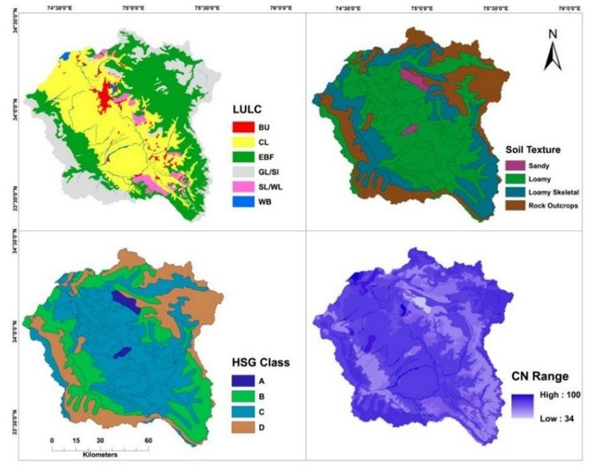
136 2010; Meraj et al. 2015; Ray et al. 2009; Romshoo et al. 2012). The total geographical area of India

137 prone to the flood is approx. 45.640 million hectares, out of which about 0.514 million hectares

138 area lie in the Jammu and Kashmir i.e. 2.3 % of its total geographical area (Planning Commission

139 2011). Climate change has increased the frequency of intense rainfall and flood events around the

140 globe including the North-West Himalayas (Mishra & Srinivasan 2013; Murari et al. 2001; IPCC

141 2007; Dhote et al. 2018; Nikam et al. 2018; Romshoo et al. 2018; Thakur et al. 2019). The history

142 revealed that in the past, Kashmir valley has encountered many causalities that caused loss of

143 livelihood and properties (Singh and Kumar 2013; Meraj et al. 2015) due to the major flood events

144 (as 879 AD, 1841, 1893, 1903, 1929, 1948, 1950, 1957, 1959, 1992, 1996, 2002, 2006, 2010, 2014

145 etc.,) ( Romshoo et al. 2018), landslides, earthquakes and avalanches (Lawrence 1895; Singh and

146 Kumar 2013). The Kashmir 2014 flood (3262.60 cumec) was similar to 1903 and 1959 floods

147 according to the people of Kashmir (Lawrence 1895; Bhatt et al. 2017; Romshoo et al. 2018) . The

148 heavy and intense rainfall from 1st Sep 2014 to 6th September 2014 led to the worst flood in the

149 Kashmir valley (Kumar and Acharya 2016; Romshoo et al. 2018). The current study emphasizes

150 on the combined utilization of hydrological modelling and indicator-based methods to assess the

151 sub-basins level flood vulnerability in the Jhelum River basin.

152

153 2. Study area and data

154 2.1 Description of the study area: Jhelum River basin

155 Fig. 1 depicts the geographical location of Jhelum river basin (9,472.14 Km2) with an outlet at the

156 Asham, Bandipora district of Jammu and Kashmir. Jhelum River originates from the spring called

157 ‘Chasma Verinag’ lies in the Anantnag district. It is commonly known as Hydaspes in Greek,

158 Vitasta in Sanskrit and Vyath in Kashmir. Jhelum River, a major tributary of Indus River acts as a

 7

159 ridge rope for the livelihood of Kashmir valley. The Jhelum River basin system comprises of

160 various tributaries, some of them flow from the Pir Panjal range and join the river on left bank while

161 remaining meet the river on right bank, draining from the Himalayan range. High elevation

162 difference can be observed in the basin varying from 1550 to 5347 m. The bowl shape of Kashmir

163 valley is filled with alluvium having steep slopes that may lead to disastrous flood, post heavy

164 rainfall storm of 1-2 hours (Dhar et al. 1982; Ganjoo 2014; Kumar and Acharya 2016).The

165 reclamation of floodplains and low lying areas for the urbanization and agriculture due to the

166 increased population density have increased the flood risk in the Jhelum basin (Census of India

167 2011; Romshoo et al. 2012). The prominent Land Use and Land covers (LULC) and soil types are

168 the measure of surface flow present in the valley, governing the sub-basins flow in the basin. The

169 region has varied LULC types such as Built-up (BU-2.19%), Crop Land (CL-37.51%), Evergreen

170 Broadleaves Forest (EBF-34.40%), Waterbody (WB-1.94%), Glacier/Snow-Ice (GL/SI-20.62%),

171 and Shrubland/Wasteland (SL/WL-3.34%), see Fig.3 and Fig.4. The percentage of Hydrological

172 Soil Group (HSG) in the study area as A-48.78%, B-25.32%, C-24.42%, and D-1.48%, depict the

173 primarily soil types in the region, see Fig.4.

174 The average annual precipitation in the valley is about 650 mm, as far as the outer hilly region

175 concerned, it receives more than the central valley (Ahmad et al. 2018). The mean temperature in

176 the valley varies from 7.5o Celsius in the winter to 19.8o Celsius in the summer season (Bhat et al.

177 2019). The Kashmir valley receives the heavy snowfall in mountainous regions and rainfall in the

178 adjoining plain areas due to two types of meteorological systems named as the barotropic southwest

179 monsoon and baroclinic extra tropical western disturbances ( Sikka 1999; Dhar and Nandargi 2005;

180 ). These disturbances repeat approximately 4 to 5 times per month during monsoon and nearly 6 to

181 7 times per month in winter (Nandargi and Dhar 2011; Kumar and Acharya, 2016). The more

 8

182 activeness of western disturbances in the winter and spring seasons as compare to summer results

183 into the most amount of precipitation during winter and spring (Bhutiyani et al. 2010; Dar et al.

184 2015).

185

186 Fig. 1. Jhelum River basin with outlet, drainages, sub-basins & gauging sites

187

188 2.2 Data and tools used

189 The Advanced Land Observing Satellite (ALOS) Phased Array type L-band Synthetic Aperture

190 Radar (PALSAR) Radiometrically Terrain Corrected (RTC) Digital Elevation Model (DEM)

191 acquired from the Alaska Satellite Facility was used in the present study for the DEM hydro-

192 preprocessing. The Indian Space Research Organisation-Geosphere Biosphere Program (ISRO-

193 IGBP) 2005, LULC and the National Bureau of Soil Survey and Land Use Planning (NBSSLUP),

194 soil data were used to prepare the Curve Number (CN) Map. The gridded daily rainfall of Indian

195 Meteorological Department (IMD) of the monsoon seasons (1992, 1997, and 2014) were used as

196 the meteorological input in the hydrological model to simulate the flood hydrographs. Tropical

197 Rainfall Measuring Mission (TRMM) 3-hourly rainfall (Sep 2014) was also used in this study to

198 find the basin lag or lag time (Tlag) in the river flow induced after the heavy rainfall event of Sep

199 2014. The observed discharge of three gauging stations i.e. Sangam, RamMunshi Bagh and Asham

200 was procured from the Irrigation and Flood control Department, Jammu and Kashmir for calibration

201 and validation of the model. The detail overview of database used in the present study is shown in

202 the Table 1. Tools and software used in the study for the processing of input data are as: (1) HEC-

203 Geospatial Hydrologic Modeling System (GeoHMS): an extension of ArcGIS 10.3 used for the

204 DEM hydro processing and the generation of basin characteristics to create the setup files for the

 9

205 HEC-HMS 4.3, (2) HEC-HMS 4.3: used for the simulation, calibration, sensitivity, and the

206 validation analysis of the model, Arc-GIS 10.3 and Erdas Imagine 2014: used for creating the

207 geospatial environment for the processing the GIS vector and raster image data, respectively.

208

209 Table 1: Datasets used in the study

210

211 3. Methodology

212 The methodology adopted to assess sub-basin level flood vulnerability is divided into two primarily

213 sections: (1) setup of hydrological model to extract sub-basin characteristics and flood peak

214 estimation; (2) identification of vulnerable sub-basins by relating flood peak discharge with sub-

215 basin characteristics using indicator-based GIS method. The outline of implemented methodology

216 is shown in Fig.2. The above two sections have been briefly explained in following subsections.

217

218 Fig. 2. Methodology flowchart

219

220 3.1 Hydrological modeling using HEC-HMS

221 3.1.1 Basin characteristics estimation using HEC-GeoHMS

222 The HEC-Geo HMS interface, an extension of ArcGIS 10.1 was used to establish semi-distributed

223 framework (Feldman 2000; ESRI 2011) for the Jhelum River basin. The user-friendly interface

224 allows the easy generation of basin characteristics for the hydrological model using topographic

225 data. The ALOS PALSAR RTC product was pre-processed that includes the processes such as fill

226 sink, flow direction, flow accumulation, stream definition, stream link, catchment grid delineation,

227 catchment polygon processing, drainage line processing and adjoint catchment processing. The

 10

228 eight direction (D8) flow model algorithm was used for the preparation of flow direction (Jenson

229 and Domingue 1988). The threshold value used for defining the streams was 100 km2, the stream

230 network was able to mimic the actual drainage pattern as seen in the satellite imagery. The gauging

231 station Asham was defined as an outlet to delineate the Jhelum River basin. For each sub-basin

232 different catchment characteristics were estimated such as river slope, river length, basin slope,

233 longest flow path, basin centroid and centroid longest flow path.

234

235 3.1.2 Hydrological model (HEC-HMS) configuration

236 The extensively used hydrological model HEC-HMS, developed by the U. S. Army Corps of

237 Engineers Hydrologic Engineering Center was used to simulate flood hydrographs in Jhelum River

238 basin ( Engineers 2008). In order to run the simulation, the model is needed to be configured with

239 well-defined processes such as (1) estimation of initial abstraction/loss (loss model), (2)

240 transformation of excess rainfall into Unit Hydrograph (UH) (transform model), (3) conversion of

241 Direct Runoff Hydrograph (DRH) into flood hydrograph (base flow model), and (4) generation of

242 flood hydrographs at various river sections (routing model); the execution of these processes depend

243 on the algorithms given in the model (Feldman 2000; Scharffenberg and Fleming 2006;).

244 The Soil Conservation Service (SCS)-Curve Number (CN) method was opted for the loss model to

245 estimate the accumulated rainfall excess (Mishra et al. 2004; Soulis and Valiantzas 2012; Prakash

246 and Abhisek 2016; Koneti et al. 2018). The SCS-CN method for the computation of accumulated

247 precipitation excess in the form of stream flow volume depends (Ibrahim-Bathis and Ahmed 2016)

248 on the soil cover i.e. HSG, cumulative rainfall, antecedent moisture and land use. SCS has

249 developed the empirical relationship between initial abstraction (Ia) and potential maximum

250 retention (S) (equation 1) (NRCS 1986).

 11

( − ) 
251 = ( − )+ 
 (1)

252 where:

253 Pe = accumulated precipitation excess at time t

254 P = accumulated rainfall depth at time t

255 Ia = the initial abstraction (initial loss)

256 S = potential maximum retention

257 = . (2)

 ( − . ) 
258 = ( − . )+ 
 (3)

259 where,

260 P ≥ 0.2S

261 = − (4)
 
262 The depression storage, interception and the infiltration during early stage of storm constitute the

263 initial abstraction (Ia) (Ponce 1994). The imperviousness of the region controls the amount of initial

264 abstraction. More is the built-up percent, more is the imperviousness and less will be the amount of

265 initial abstraction and the impervious percent of each sub-basin was calculated by the percent of

266 LULC present (NRCS 1986; Garg et al. 2017). The sub-basin wise LULC percent statistics, depict

267 the high built percent in sub-basin W910 that clearly signifies its high impervious percent and

268 hence, less initial abstraction in this sub-basin (Fig.3.). The potential maximum retention is a

269 potential measure of basin for the extraction and retention of the storm precipitation depends on the

270 CN. The mean CN value for each sub-basin was extracted from the CN raster grid as shown in the

271 Fig. 4. The CN raster was generated by the integration of soil (HSG), LULC and slope in the HEC-

 12

272 GeoHMS interface of Arc-GIS. The CN values of different LULC classes in HSG were taken from

273 the standard table called CN look up table as given in the Table 2 (NRCS 1986; Schwab et al. 2005).

274 HSG characterizes the soil types into four classes i.e., A, B, C, and D based on their hydrological

275 properties (runoff, infiltration, etc.), where D represents the soil having maximum surface runoff

276 and minimum infiltration capacity, A is the soil with minimum surface runoff and maximum

277 infiltration capacity, but C, and D, soil types lie in between A and D, respectively (NRCS 1986;

278 Subramanya 2008).

279

280 Fig. 3. LULC percent of each sub-basin

281

282 Table 2: CN values for different HSG group according to United States Department of Agriculture

283 (USDA) TR 55

284

285 The rainfall excess obtained from the loss model was transform into the surface runoff using the

286 SCS UH technique in the transform model (Feldman 2000; Reshma et al. 2010; Hari et al. 2011).

287 The mathematical formulation of SCS UH states that the peak of UH is a function of watershed

288 area and time of peak (Tp). The time of peak depends on the excess precipitation and Tlag, whereas

289 the lag time is a function of time of concentration or travel time (Tc) (NRCS 1986; Feldman 2000).

290 The TR-55 working sheet obtained during the configuration of model involves the calculation of

291 Tc. The Tc of each sub-basin is the sum of travel time obtained during the sheet flow, shallow

292 concentrated flow and channel flow that depends on the basin physical characteristics. The details

293 of the watersheds characteristics involved in the TR-55 working sheet such as sheet flow

294 characteristics, shallow concentrated flow characteristics and channel flow characteristics are

 13

295 discussed in the USDA and National Resource Conservation Soil (NRCS) TR-55 technical release

296 (NRCS 1986). The DRH peak derived from the transform model was converted into the peak of

297 flood hydrograph using the base flow model. The base flow is the delayed sub-surface flow occurs

298 above the Ground Water Table (GWT) was estimated by Straight Line method (Subramanya 2008).

299 Muskingum Cunge and lag method were opted in routing model to derive the flood hydrograph at

300 the various sections of the reach (Feldman 2000; Subramanya 2008; Hari et al. 2011; ). Muskingum

301 Cunge method is a hydraulic method of routing which involves the continuity and the momentum

302 equation along with the equation of motion of unsteady flow i.e. St. Venant equation, whereas lag

303 method routes the flow with the Tlag provided in the specific reaches before the stations (Feldman

304 2000; Subramanya 2008; Reshma et al. 2010). Tlag is the time difference in the peak of rainfall and

305 peak of discharge of the event (or delay in the event peak flow) (Subramanya 2008).

306

307 Fig. 4. LULC, Soil, HSG and CN Map of Jhelum basin

308

309 3.1.4 Construction of meteorological forcings and the simulation run

310 The meteorological forcing is one of the most important controlling indicators that governs the

311 hydrological model. The rainfall was acquired from IMD for the monsoon seasons (June-

312 September) of the year 1992, 1997, and 2014. The configured hydrological model was simulated

313 using constructed meteorological forcing for the calibration and validation. The current research

314 carried out simulations for the monsoon periods of the years 1992, 2014, and 1997 where, the model

315 calibration was done for the year 2014 and validation for the years 1992 and 1997, respectively.

316 The flood peaks discharges were estimated for each sub-basin using 2014 extreme rainfall as input

317 forcing.

 14

318

319 3.2 Identification of vulnerable sub-basins using indicator-based GIS method

320 This section includes the framework for spotting the vulnerable sub-basins. In order to locate such

321 sub-basins, the current framework is divided into two segments: 1) vulnerability approach, and

322 2) threshold selection criteria to classify the sub-basins into low and highly vulnerable.

323

324 3.2.1 Vulnerability approach

325 It is the two-steps approach: 1) the estimation of normalized scores (0-1) of vulnerability

326 indicators and sub-indicators using the functional relationship (positive and negative) between

327 the vulnerability and their indicators, and 2) the computation of sub-basin wise vulnerability.

328 Normalization is the process of making quantities comparable to each other by making them

329 unitless and rescaling to the same range (in this case, 0-1), since initially all the indicators have

330 different units and scale (Yoon 2012; Žurovec et al. 2017).

331 The present work had used an internationally recognized Human Development Index (HDI),

332 United Nation Development Program (UNDP’s), 2006 (Birkmann 2006; Xs et al. 2006) min-max

333 linear transformation, a deductive approach for the computation of normalized scores of

334 vulnerability indicators and sub-indicators (Wu et.al. 2002; Yoon 2012; Cutter et.al. 2003).

335 Previous studies have also revealed the existence of this adopted methodology framework for the

336 assessment of vulnerable areas in the different scientific fields (Yoon 2012; Behanzin et al. 2016;

337 Kumar et al. 2016; Žurovec et al. 2017; Choudhary and Badal 2018). In this approach, the

338 functional relationship is based on the theoretical understandings only, where the positive and

339 negative relation signifies the direct and inverse relation (Wu et al. 2002; Cutter et al. 2003; Yoon

340 2012). In this case, sub-basins characteristics (terrain, hydrological, land use and soil) that have

 15

341 direct or inverse relation with the sub-basins flood peaks were treated as vulnerability indicators

342 to establish the functional relationship with the vulnerability. Since, more is the food peak, more

343 will be the sub-basins vulnerability. Further, these characteristics were classified into the sub-

344 characteristics that help in demonstrating a strong theoretical functional relationship

345 understanding with vulnerability than the previous one. Slope and elevation are terrain

346 characteristics have positive (or direct) relation with the flood peaks (Cunge 1969; NRCS 1986;

347 Subramanya 2008; Yalcin 2020). CN, Long Period Average (LPA) rainfall (1970-2015), peak

348 discharge (flood peaks at Sangam, RamMunshi Bagh and Asham are 10, 100 and 200 years return

349 period, respectively during Jhelum 2014 flood events) (Bhat et al. 2019) per unit area, and CN

350 belong to the hydrological characteristics have positive relation with flood peaks except Tc that

351 has negative (or inverse) relation (NRCS 1986; Bosznay 1989; Ponce 1994; Stewart et al. 2012;).

352 Land Use characteristics such as BU, WB and GL/SI have positive relation with flood peaks

353 where EBF, CL, and WL/SL have negative relation that depends on the imperviousness of the

354 LULC ( Subramanya 2008; Brody et al. 2014; Sanyal et al. 2014; Garg et al. 2017; Mousavi and

355 Rostamzadeh 2019). For soil characteristics HSG A, B, C, and D were considered where A and

356 B have negative relation, but C and D have positive relation with the flood peaks (NRCS 1986;;

357 Kim and Lee 2008; Stewart et al. 2012; Costache et al. 2020). Characteristics and sub-

358 characteristics of sub-basins and their relationships with the flood peaks are shown in Table 3.

359 Selection criteria for these characteristics were based on the data availability and the scientific

360 literature reviews (Subramanya 2008; D’Asaro and Grillone 2012; Sanyal et al. 2014; Yan et al.

361 2015; Abdulkareem et al. 2018; Jaafar et al. 2019; Mousavi and Rostamzadeh 2019; Sadek et al.

362 2020; Costache et al. 2020).

363

 16

364 Table 3: Basin characteristics and their relationship with peak runoff

365

366 HDI, UNDP’s, 2006, mix-man linear normalization method for the positive and negative function

367 relationships of vulnerability indicators with vulnerability (Birkmann 2006; Xs et al. 2006; Yoon

368 2012) are discussed in the equations 5 and 6, respectively.

 − 
369 = − 
 (5)

 − 
370 = − 
 (6)

371 where,

372 stands for the normalized vulnerability score regarding sub-indicators (i) for the sub-basins

373 (j);

374 stands for the observed value of the same component for the same sub-basins;

375 and stand for the maximum and minimum value of the observed range of values

376 of the same component for all the sub-basins.

377 The obtained normalized values of the sub-characteristics were averaged for each sub-basin to

378 obtain normalized score of the sub-basins characteristics as:

 ∑ 
 
379 = 
 (7)

380 where,

381 being the average index of each sub-basin’s vulnerability elements, = the sum of the index

382 and = the value of the index.

383 The overall Vulnerability Index (VI) scores (Fig.10) for each sub-basin was calculated by

384 weightage linear sum of sub-basins indicators:

385 = ∑ (8)

 17

386 where,

387 is the averaged normalized score of each basin’s characteristics and is their weights used in

388 this research.

389 In this case, equal weightage (Wi = 0.25) were given to the basins characteristics to identify the

390 dominant basins characteristics also without any unfairness. Hence, the high averaged normalized

391 score values of the basin characteristics will represent their most dominant parameters influencing

392 their respective flood peaks. Higher the VI scores of sub-basins, the chance of their vulnerability

393 will be more (Birkmann 2006; Behanzin et al. 2016). The final obtained VI scores of the sub-basins

394 were used to produce the vulnerable sub-basin map (Fig.12a) using the Arc-GIS software by

395 converting the vector into polygon.

396 Identification of vulnerable districts (Fig.12b) were also done using the area percent contribution

397 of vulnerable sub-basins to each district and the calculated VI scores of respected districts shown

398 in the Table 7 and Fig. 13, respectively. The VI scores for each district ( ) was calculated using

399 the area weightage method.

400 = ∑ (9)

401 where,

402 = area percent of low or highly vulnerable sub-basins of the respective district

403 = VI scores of low or highly vulnerable sub-basins of the respective district

404

405 3.2.2 Threshold criteria

406 The current section emphasized the methods adopted for deciding the threshold VI score to classify

407 the sub-basins between low and highly vulnerable. Present research has used three different

408 scientific techniques for this purpose such as: 1) Mean method, 2) Natural breaks (Jenks) method,

 18

409 and 3) Standard deviation method, respectively to find the Optimal Threshold Value (OTV) (Chung

410 and Lee 2009; Bhattacharya et al. 2020; Singh et al. 2020), a minimum value above which the

411 maximum of given regions become vulnerable. In this case, VI score (0.457) is considered as OTV

412 (derived from the standard deviation method), see Fig.11 for the classification of sub-basins into

413 low and highly vulnerable (Fig.12).

414 Mean method of finding OTV is the average of the all the obtained data values. But Jenks (1967)

415 natural breaks classification is the method for best arrangement of values into different classes

416 identifies the breakpoints by looking for groups and patterns inherent in the data(Ayalew 2004;

417 Stefanidis and Stathis 2013; Balasubramanian et al. 2017). It minimizes and maximizes the average

418 deviation of each class from the class mean and from the other groups means, respectively i.e.

419 minimize the variance within the class but maximize the variance between classes (Jenks, 1967).

420 Standard deviation method is based on the normal distribution signifies the extent of diversion of

421 attribute’s values from mean of all the values that creates the class breaks with an equal proportion

422 of standard deviation generally one, one-half, one-third, and the one-fourth using the mean and

423 standard deviation from the mean (Stefanidis and Stathis 2013; Rahadianto et al. 2015).

424

425 4. Results and discussion

426 This section discusses the calibration and sensitivity of the hydrological model, validation of the

427 model and the identification of vulnerable sub-basins by relating their flood peak and selected

428 indicators.

429

430 4.1 Calibration and validation of the hydrological model

 19

431 Calibration is the iterative process to estimate the optimized basin parameters for satisfactory

432 agreement between the simulated and observed data. But validation is a check that measures

433 accuracy of a calibrated model, closed to the real independent forcing’s. In the present study, the

434 statistical parameters such as R2, RMSE, and NSE were used as the performance criteria for the

435 calibration and validation of the model.

436

437 4.1.1. Model calibration and its sensitivity

438 Automated method was adopted using the HEC-HMS model optimization technique (Feldman

439 2000) in order to calibrate the model. The model sensitivity (Fig.5a) towards the CN continues the

440 calibration process by an adjustment of CN scaling factor with an objective to maximize the NSE.

441 CN scaling factor is the fractional amount of change in the CN value. The surface runoff obtained

442 from the calibrated model has direct relationship with the CN. The 0 CN value means that all the

443 rain will infiltrate into the ground whereas 100 CN value means all the rainfall will flow as the

444 surface runoff that signifies the ideal pavement condition. Ideally, the CN value cannot be greater

445 than 98, since the surface will hold some little amount of rainfall (Halwatura and Najim 2013).

446 In this study, optimization trial run was implemented at the Sangam gauging station for the duration

447 similar to model simulation run (Jun 2014 to Oct 2014), but the optimization objective run was

448 scheduled daily for the event period during Sep 3, 2014 to Sep 15, 2014 against the daily observed

449 available during that period only to derive the optimized CN scaling factor. Optimized CN scaling

450 factor was then adjusted to derive the maximum NSE for the whole period of model simulation run

451 (2014) to achieve the goal of calibration at the Sangam gauging station.

452 Fig.5a depicts sensitivity of the calibrated model with the maximum NSE value 0.989 obtained

453 against the final optimized CN scaling factor, 0.98, governs the good efficiency of the model.

 20

454 Correlation coefficient (R2) of calibrated model obtained at the Sangam gauging station is 0.9935

455 (Fig.5c) signifies the good fit and the calibration curve between the observed and the simulated.

456

457 Fig.5. Calibration (2014) at Sangam: a) Model Sensitivity, b) Time Series, and c) Scattered plot

458

459 Fig.5c shows that the slope (0.9908) of the regression line at the Sangam is less than one has the

460 minimal shift towards observed discharge with respect to the 450 line, signifying that the model is

461 under predicting at Sangam. The calibrated peak flow simulated at the Sangam is 3425.90 m3/s

462 (Fig.5b) with -5.01 relative peak error percent. RMSE obtained for the calibrated model during the

463 linear regression at the Sangam gauging station is 106.53 m3/s. Calibrated outflow from the Sangam

464 is now the inflow for the other stations such as RamMunshi Bagh and Asham in its downstream.

465 CN of the sub-basins contributing to these two stations in the downstream are also optimized to

466 obtain the good fit and calibration curves (Fig.6a and 6b) between the observed and the simulated

467 at these sites. The maximum NSE obtained during this correlation process at the RamMunshi Bagh

468 and Asham is 0.8437 and 0.7368. R2 values 0.9588 and 0.9941 obtained during the correlation at

469 RamMunshi Bagh and Asham, respectively shows the good fit curve. Model is over predicting at

470 the RamMunshi Bagh and Asham since the shift in the regression line is towards the simulated one

471 from the 450 line, having slopes (1.1481 and 1.2822) greater than 1. RMSE obtained at the

472 RamMunshi Bagh and Asham during the whole process of regression is 187.75 m3/s and 78.60

473 m3/s.

474

475 Fig.6. Scattered plots (2014) at other stations: a) RamMunshi Bagh and b) Asham

476

 21

477 4.1.2 Diversion and attenuation of the flood peak

478 This section enlightened the monitoring the capacity of reaches and the constructed Flood Spill

479 Channel (FSC). However, FSC starts at Reduced Distance (RD) 68.64 km Jhelum River and FSC

480 RD 0 km in between the Padshahi Bagh (RD 66.93 km Jhelum River) and RamMunshi Bagh (RD

481 71.70 km Jhelum River) gauging sites, respectively (Fig.2). While ends at the confluence point of

482 FSC and Ferozpora (Kuzer branch) Nallah at FSC RD 32.62 km, respectively somewhere nearer to

483 the downstream of Asham gauging site (RD 106.10 km), see Fig.2. The section also monitors the

484 cause of attenuated peaks observed during the 2014 flood events, either it is due to diversion from

485 FSC or due to the reduction in the capacity of FSC and reach or both. The diversion in peak

486 discharge was also observed during the Jhelum 2014 flood from the (FSC) situated between the

487 Padshahi Bagh (RD 66.93 km) and RamMunshi Bagh (71.70 km) gauging sites. According to

488 Irrigation and flood control department, Kashmir the maximum observed diverted peak from the

489 FSC was 244 m3/s (8,600 cusec), 10.61% of peak at Padshahi Bagh (2299 cumec) gives the current

490 capacity of the FSC during 2014 (Eptisa 2018; Romshoo et al. 2018). Diversion structure added

491 between the Padshahi Bagh and RamMunshi Bagh in the configured calibrated model simulated

492 the diverted peak flow as 223.16 cumec with relative percentage error 8.54 % at the same capacity

493 of FSC observed during the 2014 flood. The details about the diversion from the FSC during the

494 Jhelum 2014 flood are discussed in the Table 4. During 2014, with respect to the inflow from the

495 Sangam (3262.61 Cumec), the maximum percentage of flow diverted from the FSC was also only

496 10.61% (244 Cumec) of Padshahi Bagh. Maximum diversion in the peak flow observed from the

497 FSC with respect to the inflow from the Sangam (peak flow 1834.08 Cumec & 1780.44 Cumec)

498 during the event years 1992 and 1997 were 36.81% & 45.17 %.

499

 22

500 Table 4: Diversion of peak discharge during Jhelum 2014 flood

501

502 It was found that observed time lag (Fig.6.) in the peaks occurred at the gauging sites in the reach

503 during the Jhelum 2014 flood. Fig.6a. shows the approx. 11 hrs. (660 min) Tlag was observed at the

504 Sangam gauging location situated in the upstream of the Jhelum. Since, according to Central Water

505 Commission (CWC), the India Standard Time (IST) for starting the discharge data recording at the

506 gauging sites is 8:00 AM (CWC 2017), where 00:00 hrs. represent 12:00 AM. It was observed that

507 RamMunshi Bagh and Asham gauging sites have also Tlag 59 hrs. (2 days 11 hrs.), and 75 hrs. (3

508 days 3 hrs.), respectively with respect to the Sangam as depicted in the Fig.6b. T lag at Asham

509 gauging station with respect to the RamMunshi Bagh was observed as 18 hrs. (108 min), see Fig.6b.

510 The reduction in the outflow peaks at the gauging locations, called attenuation (Subramanya 2008)

511 were also found in this study during the Jhelum 2014 flood event. Table 5 shows the attenuations

512 observed in the peaks at the respective gauging stations during 2014 flood event. Total 37.02% and

513 34.41% attenuation in the peaks of outflow at RamMunshi Bagh and Asham were found, with

514 respect to their respective recorded inflows in their upstream. The outflow at Asham has 58.61%

515 attenuation in its peak with respect to the inflow recorded at Sangam. Attenuation in the peak

516 discharge were also found in the observed flow during the event year 1992 at RamMunshi Bagh

517 and Asham by 36.81% and 0.55%, respectively with respect to the inflows from their respective

518 upstream reaches, where 1152.49 Cumec measured at Asham. During the year 1997, the attenuated

519 peak was also observed at both RamMunshi Bagh (976.13 Cumec, 45.17%) and Asham (824.30

520 Cumec, 15.55%).

521

522 Fig.7. a) Time lag (2014) at Sangam; b) flow (2014) at Sangam, RamMunshi Bagh & Asham

 23

523

524 Table 5: Reach lag and attenuation in the outflow at the gauging stations during Jhelum 2014 flood

525

526 4.1.3. Model validation

527 The calibrated configured model is needed to be validated for checking the stability of the

528 calibrated model (Halwatura and Najim 2013). In the current research, the model was validated

529 at the Sangam gauging site (Sangam in the upstream has higher contribution percent in the flood

530 peaks than RamMunshi Bagh and Asham in the downstream, see Fig.11 and Table 6 and 7) for

531 the monsoon seasons of the years 1992 and 1997. Since during the monsoon period of selected

532 validation years, the valley has also experienced the extreme flood events (Romshoo et al. 2018),

533 see Fig.8. The statistical analysis of model validation results (see Fig.9) that manifest the good

534 agreement of the calibrated model in predicting the real scenario in the studied basin. Correlation

535 coefficient values obtained 0.9618 and 0.9486 exhibit good linear fitting of regression line during

536 the years 1992 and 1997. Obtained slope values 0.9882 and 1.0210 for the years 1992 and 1997

537 show the shifting of regression line towards the observed and simulated, respectively. Also, the

538 RMSE obtained for the regression analysis are 86.39 Cumec and 79.64 Cumec, respectively.

539

540 Fig.8. Year wise maximum flow at Sangam

541

542 Fig.9.Validation scattered plots at Sangam: a) year 1992 and b) year 1997

543

544 4.2 Flood vulnerability assessment of the sub-basins

 24

545 The present section of the results and discussion highlights the vulnerable sub-basins that have

546 significant contribution to their flood peaks. The most dominant indicators of such sub-basins

547 influencing their flood peaks were also identified during the recognition process of these sub-basins

548 of the Jhelum River. The normalized scores of the basin characteristics and the VI score obtained

549 for each sub-basin are shown in Fig.10. It is observed that W810 (VI score - 0.645) and W950 (VI

550 score - 0.325) sub-basins are the most and the least vulnerable (Fig.12a and Table 6) sub-basins of

551 the Jhelum river contributing to the Sangam and RamMunshi Bagh gauging sites situated in the

552 upstream and downstream, respectively.

553

554 Fig.10. Sub-basins wise Vulnerability Index score plot with their classification using the color ramp

555 representation and the normalized score plot of their characteristics

556

557 Fig.11. D/S = Downstream (contributing to RamMunshi Bagh and Asham) and U/S = Upstream

558 (contributing to Sangam)

559

560 The sub-basins which has VI score below the obtained OTV 0.457, see Fig.11 were categorized as

561 highly vulnerable sub-basins that contributing significantly to their peak flood (Table 6). The OTV

562 for this classification was considered using the standard deviation classification method. Since,

563 among all the three adopted methods (mean, natural breaks, and standard deviation) for the OTV

564 selection, the standard deviation has minimum value and classify the maximum number sub-basins

565 of Jhelum river basin into the vulnerable category. All the highly vulnerable sub-basins of this

566 basin have benefaction to the Sangam gauging site situated in the upstream of the river except the

567 W610 which is contributing the Asham gauging station in the downstream the river. The most

 25

568 influencing characteristics of such sub-basins belong to their respective gauging sites are discussed

569 in the Table 6. The hydrological characteristics (averaged normalized score – 0.844) have

570 dominated over the terrain, soil and LULC characteristics in case of most vulnerable sub-basin

571 W810. W810 has the lowest Tc (3.66 hrs.), highest LPA (1076.63 mm), low area (228.07 Km2) and

572 high CN (76) comparison to the all other sub-basins signify its most vulnerable condition. Romshoo

573 et al. (2018) have also stated that the lower Tc and high slope gradients of sub-basins in the upstream

574 sides contributing to the Sangam are the indicators responsible for Jhelum 2014 flood event. The

575 lower Tc means the time required by the river flows to reach their respective junction will be very

576 low (Subramanya 2008). However, the dominant parameters of other highly vulnerable sub-basins

577 include the soil and terrain characteristics as well except LULC parameters. Fig.11 represents the

578 final map of the vulnerable sub-basins of Jhelum River stretched between maximum and minimum

579 VI scores 0.644 and 0.325, respectively depicts the high and the low vulnerable sub-basins.

580

581 Table 6: Sub-basins contributing significantly to the flood peak flows and their most dominant

582 influencing parameters

583

584 Fig.12. Vulnerability Index score map: a) sub-basins wise, and b) district wise

585

586 Fig.12b depicts the low and highly vulnerable sub-basins located in the respective districts.

587 Anantnag district has the largest area (2725.738 Km2) amongst the all other districts covering

588 only the highly vulnerable sub-basins (100%) namely, W610, W700, W810, W1020, W1090, and

589 W1130, respectively (Table 7 and Fig.13), place it in the category of highly vulnerable. Like the

590 Anantnag district, Ganderbal, Kulgam and the part of Ramban are also 100% covering the only

 26

591 highly vulnerable sub-basins as shown in the table 7 and Fig.13 made them highly vulnerable

592 districts. However, the Shupiyan district has both low (49.17 %) and highly (50.83%) vulnerable

593 sub-basins where the contribution of highly vulnerable is more that made the district highly

594 vulnerable. But, the VI score obtained for the district using the equation 9 as shown in Fig.13 has

595 made the Kulgam, the most vulnerable district and the Badgam as the least vulnerable. Badgam

596 and part of Baramulla have 100% contribution of only low vulnerable sub-basins however

597 Pulwama and Srinagar have both low and highly vulnerable sub-basins area covering where the

598 area percentage of low vulnerable sub-basins are high. The districts are also categorized into the

599 downstream (Badgam, part of Baramulla, Pulwama, Srinagar, and Ganderbal) and upstream

600 (Shupiyan, part of Ramban, Anantnag and Kulgam) parts, see Fig.13 based on the respective area

601 percentage of sub-basins (located in the upstream and downstream) in the districts for the easy

602 acquirement of information. Present study have used the indicator based approach for

603 vulnerability assessment using the indicators based on hydrological aspects of basin only.

604 However, the results may vary due to the use of only socio-economic indicators in this

605 vulnerability assessment. Hence, the integrated uses of hydrology and socio-economic based

606 indicators can be used for the future research in this field.

607

608 Table 7: Analysis of districts corresponds to the low and highly vulnerable sub-basins

609

610 Fig.13. Area contribution of sub-basins in the respective districts and district wise VI score

611

612 5. Conclusion

 27

613 A novel approach using hydrological model and indicator-based GIS method for sub-basin level

614 flood peak and vulnerability assessment has been proposed in this study.

615 1. The sub-basins W810 (Fig.2 and Fig.12b), part of Anantnag district, contributing to the Sangam

616 gauging site, is found to be the most vulnerable among the all other sub-basins, see Fig.12a.

617 The peak discharge of this basin was controlled by hydrological characteristics compared to

618 other characteristics (e.g. terrain, soil; Table 6).

619 2. Various districts such as Shupiyan, Ganderbal, Anantnag, part of Rambana and Kulgam are

620 falling under highly vulnerable category. However, Anantnag district (2725.738 Km2) acquires

621 the largest part of the highly vulnerable region of the Jhelum river basin, see Fig. 12b and Table

622 7.

623 3. It was found that 50% sub-basins falling in highly vulnerable category are contributing to the

624 accumulated flow of Sangam station making upstream side of Jhelum River more vulnerable

625 than the downstream side (Table 6 and 7).

626 4. Attenuation in the observed peak outflows were also observed during 2014 flood event due to

627 reduction in the carrying capacity of river channel and FSC (Table 4 and 5). The overflow of

628 discharge during that flood duration has caused the inundation in the regions surrounding to the

629 Jhelum River. The flood inundation for that flooded period was mapped by Bhatt et al. (2017)

630 using the Remote Sensing satellite data .The decrement in the capacity of the reach and the FSC

631 were due the siltation and accumulation of sediments carried by the regular and the heavy flood

632 flows.

633 5. These vulnerable sub-basins and the sub-basins with low Tc are needed to take care by the

634 flood management authorities to prevent the region from such type of flood events in the future.

 28

635 It is recommended to monitor the sediment flows along with the discharge on the regular basis in

636 the channel and the FSC to avoid the 2014 flood events like situation in the future. Authorities

637 should maintain (dredging for removing sediments) the existing FSCs and river channel regularly

638 and increase the number of FSCs especially in the downstream of Sangam to increase the capacity

639 of existing FSCs. In order to increase mitigation time during and before the extreme flood events,

640 the increment in Tc of highly vulnerable sub-basins is advised through sustainable watershed

641 management. It is recommended to use AI-based models and their hybrids in the future studies to

642 improvise the results of hydrological predictions.

643

644 Acknowledgement

645 Our heartfelt thanks to Irrigation and flood control department, Kashmir and India Metrological

646 Department for providing the discharge and rainfall data. We are also thankful to Director, Indian

647 Institute of Remote Sensing, ISRO, Dehradun and Disaster Management Support (DMS) office of

648 ISRO headquarters for their help, support and motivation during this entire research. This work was

649 done as part of ISRO sponsored DMS (research and development) project “Remote sensing, ground

650 observations and integrated modelling based early warning system for climatic extremes of North

651 West Himalayan region.”

652

653 Conflicts of interest/ Competing interest

654 The authors declare that they have no known competing financial interests or personal relationships

655 that could have appeared to influence the work reported in this paper.

656

657 Availability of data and material

 29

658 The data that support the findings of this study are available from the corresponding author Pankaj

659 R. Dhote, upon reasonable request.

660

661 Code availability

662 Not applicable.

663

664 Authors' contributions

665 RR:Conceptualization, analysis and prepared original draft; PRD: Conceptualization, analysis and

666 wrote paper; PKT: Reviewed paper and helped in producing figurers; SPA: Supervision and

667 reviewed paper

668

669 References

670 Abdulkareem, J.H., Sulaiman, W.N.A., Pradhan, B., and Jamil, N.R., 2018. Relationship

671 between design floods and land use land cover (LULC) changes in a tropical complex

672 catchment. Arab J Geosci, 11 (14), 1–17. https://doi.org/10.1007/s12517-018-3702-4.

673 Abushandi, E. and Merkel, B., 2013. Modelling rainfall runoff relations using HEC-HMS and

674 IHACRES for a single rain event in an arid region of Jordan. Water Resour Manage, 27(7),

675 2391-2409. https://doi.org/10.1007/s11269-013-0293-4..

676 Aggarwal S.P., Garg V., Thakur P.K., Nikam B.R., 2019. Hydrological Modelling in North

677 Western Himalaya. In: Navalgund R., Kumar A., Nandy S. (eds). Remote Sensing of

678 Northwest Himalayan Ecosystems. Springer, Singapore. https://doi.org/10.1007/978-981-

679 13-2128-3_6.

680 Ahmad, T., Pandey, A.C., and Kumar, A., 2018a. Flood hazard vulnerability assessment in

 30

681 Kashmir Valley , India using geospatial approach. Phy Chem Earth, Parts A/B/C, 105, 59–

682 71. https://doi.org/10.1016/j.pce.2018.02.003.

683

684 Álvarez, C., Juanes, J. a., García, A., Sainz, A., Puente, A., and Revilla, J. a., 2008. Surface

685 water resources assessment in scarcely gauged basins in the north of Spain. J

686 Hydrol, 356(3-4), 312-326. https://doi.org/10.1016/j.jhydrol.2008.04.019.

687 Ayalew, L., Yamagishi, H. and Ugawa, N., 2004. Landslide susceptibility mapping using GIS-

688 based weighted linear combination, the case in Tsugawa area of Agano River, Niigata

689 Prefecture, Japan. Landslides, 1(1), 73-81. https://doi.org/10.1007/s10346-003-0006-9.

690 Balasubramanian, A., Duraisamy, K., Thirumalaisamy, S., Krishnaraj, S., and Yatheendradasan,

691 R.K., 2017. Prioritization of subwatersheds based on quantitative morphometric analysis in

692 lower Bhavani basin, Tamil Nadu, India using DEM and GIS techniques. Arab J Geosci,

693 10 (24), 552. https://doi.org/10.1007/s12517-017-3312-6.

694 Behanzin, D.I., Thiel, M., Szarzynski, J., and Boko, M., 2016. GIS-Based Mapping of Flood

695 Vulnerability and Risk in the Bénin Niger River Valley. Int J Geomat Geosci, 6 (3), 1653–

696 1669.

697 Beyene, T., Lettenmaier, D.P., and Kabat, P., 2010. Hydrologic impacts of climate change on

698 the Nile River Basin: Implications of the 2007 IPCC scenarios. Climatic Change, 100 (3),

699 433–461. https://doi.org/10.1007/s10584-009-9693-0.

700 Bhat, M.S., Alam, A., Ahmad, B., Kotlia, B.S., Farooq, H., Taloor, A.K., and Ahmad, S., 2019.

701 Flood frequency analysis of river Jhelum in Kashmir basin. Quatern Int, 507, 288–294.

702 https://doi.org/10.1016/j.quaint.2018.09.039.

703 Bhatt, C.M., Rao, G.S., Farooq, M., Manjusree, P., Shukla, A., Sharma, S.V.S.P., Kulkarni,

 31