Air quality and health benefits from ultra-low emission control policy indicated by continuous emission monitoring: a case study in the Yangtze ...
←
→
Page content transcription
If your browser does not render page correctly, please read the page content below
Atmos. Chem. Phys., 21, 6411–6430, 2021
https://doi.org/10.5194/acp-21-6411-2021
© Author(s) 2021. This work is distributed under
the Creative Commons Attribution 4.0 License.

Air quality and health benefits from ultra-low emission control
policy indicated by continuous emission monitoring: a case study
in the Yangtze River Delta region, China
Yan Zhang1,2 , Yu Zhao1,3 , Meng Gao4 , Xin Bo5 , and Chris P. Nielsen6
1 StateKey Laboratory of Pollution Control and Resource Reuse and School of the Environment, Nanjing University,
163 Xianlin Rd., Nanjing, Jiangsu 210023, China
2 Jiangsu Environmental Engineering and Technology Co., Ltd., Jiangsu Environmental Protection Group Co., Ltd.,

8 East Jialingjiang St., Nanjing, Jiangsu 210019, China
3 Jiangsu Collaborative Innovation Center of Atmospheric Environment and Equipment Technology (CICAEET), Nanjing

University of Information Science and Technology, Jiangsu 210044, China
4 Department of Geography, State Key Laboratory of Environmental and Biological Analysis, Hong Kong Baptist University,

Hong Kong SAR, China
5 The Appraisal Center for Environment and Engineering, Ministry of Environmental Protection, Beijing 100012, China
6 Harvard-China Project on Energy, Economy and Environment, John A. Paulson School of Engineering and Applied

Sciences, Harvard University, 29 Oxford St., Cambridge, MA 02138, USA

Correspondence: Yu Zhao (yuzhao@nju.edu.cn)

Received: 4 August 2020 – Discussion started: 20 November 2020
Revised: 13 March 2021 – Accepted: 16 March 2021 – Published: 27 April 2021

Abstract. To evaluate the improved emission estimates from         of case 2, our base case for policy comparisons, would be less
online monitoring, we applied the Models-3/CMAQ (Com-              than 7 % for all pollutants. The result implies a minor bene-
munity Multiscale Air Quality) system to simulate the air          fit of ultra-low emission control if implemented in the power
quality of the Yangtze River Delta (YRD) region using              sector alone, which is attributed to its limited contribution to
two emission inventories with and without incorporated data        the total emissions in the YRD after years of pollution con-
from continuous emission monitoring systems (CEMSs) at             trol (11 %, 7 %, and 2 % of SO2 , NOX , and primary particle
coal-fired power plants (cases 1 and 2, respectively). The nor-    matter (PM) in case 2, respectively). If the ultra-low emis-
malized mean biases (NMBs) between the observed and sim-           sion policy was enacted at both power plants and selected in-
ulated hourly concentrations of SO2 , NO2 , O3 , and PM2.5         dustrial sources including boilers, cement, and iron and steel
in case 2 were −3.1 %, 56.3 %, −19.5 %, and −1.4 %, all            factories (case 4), the simulated SO2 , NO2 , and PM2.5 con-
smaller in absolute value than those in case 1 at 8.2 %,           centrations compared to the base case would be 33 %–64 %,
68.9 %, −24.6 %, and 7.6 %, respectively. The results indi-        16 %–23 %, and 6 %–22 % lower, respectively, depending on
cate that incorporation of CEMS data in the emission inven-        the month (January, April, July, and October 2015). Com-
tory reduced the biases between simulation and observation         bining CMAQ and the Integrated Exposure Response (IER)
and could better reflect the actual sources of regional air pol-   model, we further estimated that 305 deaths and 8744 years
lution. Based on the CEMS data, the air quality changes and        of life loss (YLL) attributable to PM2.5 exposure could be
corresponding health impacts were quantified for different         avoided with the implementation of the ultra-low emission
implementation levels of China’s recent “ultra-low” emis-          policy in the power sector in the YRD region. The analogous
sion policy. If the coal-fired power sector met the require-       values would be much higher, at 10 651 deaths and 316 562
ment alone (case 3), the differences in the simulated monthly      YLL avoided, if both power and industrial sectors met the
SO2 , NO2 , O3 , and PM2.5 concentrations compared to those        ultra-low emission limits. In order to improve regional air

Published by Copernicus Publications on behalf of the European Geosciences Union.
6412                                 Y. Zhang et al.: Air quality and health benefits from ultra-low emission control policy

quality and to reduce human health risk effectively, coor-            Evaluations of emission estimates and the changed air
dinated control of multiple sources should be implemented,         quality from emission abatement provide useful information
and the ultra-low emission policy should be substantially ex-      on the sources of air pollution and the effectiveness of pol-
panded to major emission sources in industries other than the      lution control measures. Air quality modeling is an impor-
power industry.                                                    tant tool for evaluating emission inventories, by comparing
                                                                   simulation results with available observation data. Developed
                                                                   by the US Environmental Protection Agency (US EPA), the
                                                                   Models-3/Community Multiscale Air Quality (CMAQ) sys-
1   Introduction
                                                                   tem has been widely used in China (Li et al., 2012; An et al.,
Due to swift economic development and associated growth in         2013; Wang et al., 2014; Han et al., 2015; Zheng et al., 2017;
demand for electricity, coal-fired power plants have played        Zhou et al., 2017; Chang et al., 2019). Han et al. (2015) con-
an important role in energy consumption and air pollutant          ducted CMAQ simulations with different emission invento-
emissions for a long time in China. For example, Zhao et           ries for East Asia and found that the simulated NO2 columns
al. (2008) for the first time developed a “unit-based” emis-       using the emission inventory for the Intercontinental Chem-
sion inventory of primary air pollutants from the coal-fired       ical Transport Experiment Phase B (INTEX-B; Zhang et al.,
power sector in China and found that the sector contributed        2009) agreed better with the satellite observations of the
53 % and 36 % to the national total emissions of SO2 and           Ozone Monitoring Instrument (OMI) than the simulations
NOX , respectively, in 2005. Subsequently, SO2 and NOX             using the Regional Emission Inventory in Asia (REAS v1.11;
emissions from the power sector were estimated to account,         Ohara et al., 2007). Zhou et al. (2017) applied CMAQ to eval-
respectively, for 28 %–53 % and 29 %–31 % of the total an-         uate the national, regional, and provincial emission invento-
nual emissions in China during 2006–2010 according to the          ries for the Yangtze River Delta (YRD) region, and the best
Multi-resolution Emission Inventory for China (MEIC; http:         model performance with the provincial inventory confirmed
//www.meicmodel.org, last access: 19 April 2021). To reduce        that the emission estimate with more detailed information in-
high emissions and improve air quality in China, advanced          corporated on individual power and industrial plants helped
air pollutant control devices (APCDs) have been gradually          improve the air quality simulation at relatively high horizon-
applied in the power sector including flue gas desulfuriza-        tal resolution. With air quality modeling, moreover, many
tion (FGD) for SO2 control, selective catalytic reduction          studies have explored the environmental benefits of emission
(SCR) for NOX control, and high-efficiency dust collectors         control measures taken in recent years (B. Zhao et al., 2013;
for primary particulate matter (PM) control. In recent years,      Huang et al., 2014; Li et al., 2015; Wang et al., 2015; Tan et
moreover, an ultra-low emission retrofitting policy has been       al., 2017). Wang et al. (2015) found that the implementation
widely implemented, seeking to reduce the emission levels          of the new Emission Standard of Air Pollutants for Thermal
of coal-fired power plants to those of gas-fired ones (i.e., 35,   Power Plants (GB13223-2011) could effectively reduce pol-
50, and 5 mg m−3 for SO2 , NOX , and PM concentrations in          lutant emissions in China, and the ambient concentrations of
the flue gas). The expanded use of associated technologies         SO2 , NO2 , and PM2.5 would decrease by 31.6 %, 24.3 %, and
has induced great changes in the magnitude and spatiotem-          14.7 %, respectively, in 2020 compared with a baseline sce-
poral distribution of emissions from the power sector, which       nario for 2010. Li et al. (2015) found that the simulated con-
have been analyzed and quantified by a series of studies (Y.       centrations of PM2.5 in the YRD region would decrease by
Zhao et al., 2013; Zhang et al., 2018; Liu et al., 2019; Tang et   8.7 %, 15.9 %, and 24.3 % from 2013 to 2017 in three sce-
al., 2019; Y. Zhang et al., 2019). With the updated unit-level     narios with weak, moderate, and strong emission reduction
information, for example, MEIC estimated that the power            assumptions in the Clean Air Action Plan, respectively.
sector shares of national total emissions declined from 28 %          Besides air quality, the health risk caused by air pollution
to 22 % and from 29 % to 21 % for SO2 and NOX during               exposures in China is a major concern, especially to PM2.5 , a
2010–2015, respectively. Incorporating data from continuous        dominant pollutant in haze conditions. Lim et al. (2012) has
emission monitoring systems (CEMSs), Tang et al. (2019)            identified air pollution as a primary cause of global burden
found that China’s annual power sector emissions of SO2 ,          of disease, especially in low- and middle-income countries,
NOX , and PM declined by 65 %, 60 %, and 72 %, respec-             and PM2.5 pollution was ranked the fourth leading cause of
tively, during 2014–2017, due to the enhanced control mea-         death in China. Studies have shown that PM2.5 is closely re-
sures. With a method of collecting, examining, and applying        lated to several causes of death (Dockery et al., 1993; Hoek
CEMS data, similarly, our previous work indicated that the         et al., 2013; Lelieveld et al., 2015; Butt et al., 2017; Gao
estimated emissions from the power sector would be 75 %,           et al., 2018; Maji et al., 2018). For example, Lelieveld et
63 %, and 76 % smaller than those calculated without CEMS          al. (2015) estimated that nearly 1.4 million people died each
data for SO2 , NOX , and PM, respectively (Y. Zhang et al.,        year due to PM2.5 exposure in China, 18 % of which were re-
2019).                                                             lated to the emissions from the power sector. Based on simu-
                                                                   lated PM2.5 using WRF-Chem (Weather Research and Fore-
                                                                   casting (WRF) model coupled with chemistry) and the In-

Atmos. Chem. Phys., 21, 6411–6430, 2021                                             https://doi.org/10.5194/acp-21-6411-2021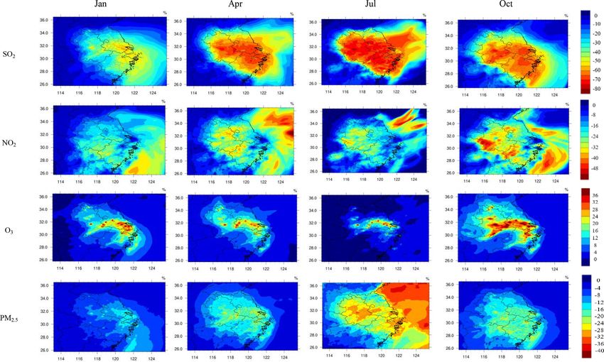
Y. Zhang et al.: Air quality and health benefits from ultra-low emission control policy                                         6413

tegrated Exposure Response (IER) model, Gao et al. (2018)
estimated that emissions from the power sector results in 15
million years of life lost per year in China. In addition to as-
sessment of health risk based on observations of actual air
pollution levels, studies have also analyzed the health ben-
efits of emission control policies (Lei et al., 2015; Li and
Li, 2018; Dai et al., 2019; Q. Zhang et al., 2019; X. Zhang
et al., 2019). Combining available observation and CMAQ
modeling, Q. Zhang et al. (2019) identified improved emis-
sion controls on industrial and residential pollution sources
as the main drivers of reductions in PM2.5 concentrations
from 2013 to 2017 in China and estimated an annual reduc-
tion of PM2.5 -related deaths at 0.41 million. Lei et al. (2015)
evaluated the health benefit of the Air Pollution Prevention
and Control Action Plan of China and found that full real-
ization of the air quality goal in this plan could avoid 89 000
premature deaths of urban residents and reduce 120 000 inpa-
tient cases and 9.4 million outpatient service and emergency
cases. Focusing more regionally, X. Zhang et al. (2019) esti-
mated the health impact of a “coal-to-electricity” policy for
residential energy use in the Beijing-Tianjin-Hebei (BTH)
region. They projected that the reduction in PM2.5 concen-
trations from the policy would avoid nearly 22 200 cases of
premature death and 607 800 cases of disease in the region in
2020. For areas with strong, industry-based economies, the
impact of air quality on public health can be more significant,
attributed both to relatively large and dense populations and
to high pollution levels. Until now, however, there have been
few studies focusing on air quality improvement and corre-         Figure 1. The modeling domain and the locations of the concerned
sponding health benefits attributed to the implementation of       provinces and their capital cities. The numbers 1–4 represent the
the latest emission control policies, notably China’s ultra-low    cities of Nanjing, Hefei, Shanghai, and Hangzhou, respectively. The
emission policy introduced above, at a regional scale.             map data, provided by the Resource and Environment Data Cloud
   As one of the most densely populated and economically           Platform, are freely available for academic use (http://www.resdc.
developed regions, the YRD region encompassing Shanghai            cn/data.aspx?DATAID=201, last access: 19 April 2021), © Insti-
and Anhui, Jiangsu, and Zhejiang provinces is a key area for       tute of Geographic Sciences & Natural Resources Research, Chi-
air pollution prevention and control in China (Huang et al.,       nese Academy of Sciences.
2011; Li et al., 2011, 2012). It is also one of the regions with
the earliest implementation of the ultra-low emission policy
on the power sector in the country. Quantification of emis-        2     Methodology and data
sion reductions as well as subsequent changes in air quality
is crucial for full understanding of the environmental benefits    2.1    Air quality modeling
of the policy. To test the possible improvement in the regional
emission inventory, this study evaluated the air quality mod-      In this study, we adopted CMAQ version 4.7.1 (UNC, 2010)
eling performance without and with CEMS data incorporated          to conduct air quality simulations and to evaluate various
in the estimation of emissions of the coal-fired power sector      emission inventories for the YRD region. The model has per-
for the YRD region. The changes in regional air quality and        formed well in Asia (Zhang et al., 2006; Uno et al., 2007; Fu
health risk resulting from the implementation of the ultra-low     et al., 2008; Wang et al., 2009). Two one-way nested domains
emission policy for key industries were quantified combin-         were adopted for the simulations, and the horizontal resolu-
ing the air quality modeling and the health risk model. The        tions were set at 27 and 9 km square grid cells, respectively,
results provide scientific support for incorporation of online     as shown in Fig. 1. The mother domain (D1, 177 × 127 cells)
monitoring data to improve the estimation of air pollutant         covered most of China and all or parts of surrounding coun-
emissions and for better design of emission control policies       tries in east, southeast, and south Asia. The second model-
based on their simulated environmental effects.                    ing region (D2, 118 × 121 cells) covered the YRD region,
                                                                   including Jiangsu, Zhejiang, Shanghai, Anhui, and parts of
                                                                   surrounding provinces. Lambert conformal conic projection

https://doi.org/10.5194/acp-21-6411-2021                                             Atmos. Chem. Phys., 21, 6411–6430, 2021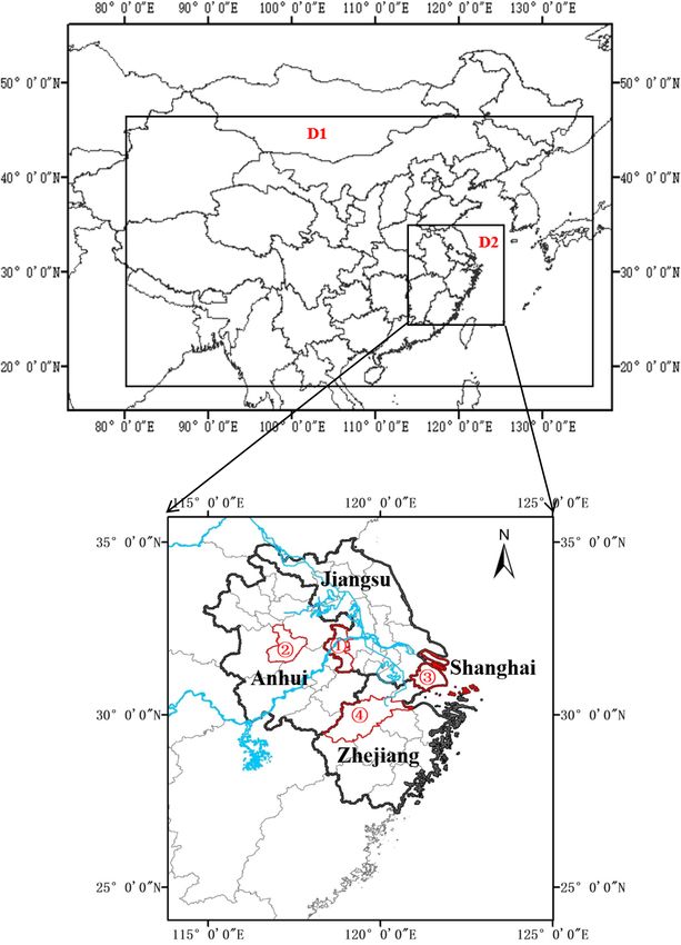
6414                                Y. Zhang et al.: Air quality and health benefits from ultra-low emission control policy

was applied for the entire simulation area centered at 34◦ N,     (Xia et al., 2016). The total emissions excluding those of the
110◦ E with two true latitudes (40◦ N and 25◦ N). The simu-       power sector of SO2 , NOX , and PM for the YRD region were
lated periods were January, April, July, and October 2015, as     estimated at 1501.0, 3468.4, and 2711.2 Gg for 2015, respec-
representative of the four seasons. The first 5 d in each month   tively. The emission inventory in Xia et al. (2016) was de-
were set as a spin-up period to provide initial conditions        veloped using activity data at the provincial level, and the
for later simulations. The Carbon Bond gas-phase mecha-           spatial distribution of emissions by sector was conducted ac-
nism (CB05) and AERO5 aerosol module were adopted in              cording to that of MEIC with the original spatial resolution
all the CMAQ modules, with details of the model configura-        of 0.25◦ × 0.25◦ in this study. The gridded emissions were
tion found in Zhou et al. (2017). The initial concentrations      further downscaled to horizontal resolutions of 27 and 9 km
and boundary conditions for the D1 mother domain were the         in D1 and D2, respectively, based on the spatial distribu-
default clean profile, while they were extracted from CMAQ        tion of population (for residential sources), industrial gross
outputs of D1 simulations for the nested D2 domain. Nor-          domestic product (for industrial sources), and the road net-
malized mean bias (NMB), normalized mean error (NME),             work (for on-road vehicles). The monthly variations of emis-
and the correlation coefficient (R) between the simulations       sions from each sector were assumed to be the same as in
and observations were selected to evaluate the performance        MEIC. Constrained by available ground observation, a larger
of CMAQ modeling (Yu et al., 2006). The hourly concen-            monthly variation in the emissions of black carbon aerosols
trations of SO2 , NO2 , O3 , and PM2.5 were observed at 230       was found for the central YRD region than that in MEIC.
state-operated ground stations of the national monitoring net-    Limited improvement in air quality model performance was
work in the YRD region and were collected from Qingyue            consequently achieved, implying that the bias from the tem-
Open Environmental Data Center (https://data.epmap.org,           poral variation was insignificant (Zhao et al., 2019). In addi-
last access: 19 April 2021).                                      tion, the Model Emissions of Gases and Aerosols from Na-
   The Weather Research and Forecasting (WRF) Model ver-          ture modeling system developed under the Monitoring Atmo-
sion 3.4 (http://www.wrf-model.org/index.php, last access:        spheric Composition and Climate project (MEGAN-MACC;
19 April 2021; Skamarock et al., 2008) was applied to pro-        Guenther et al., 2012; Sindelarova et al., 2014) was applied
vide meteorological fields for CMAQ. Terrain and land-use         as the biogenic emission inventory, and the emissions of
data were taken from global data of the US Geological Sur-        Cl, HCl, and lightning NOX were obtained from the Global
vey (USGS), and the first-guess fields of meteorological          Emissions InitiAtive (GEIA; Price et al., 1997).
modeling were obtained from the final operational global             For the power sector in the YRD region specifically, we
analysis data (ds083.2) by the National Centers for Environ-      adopted the unit-level emission estimates from our previ-
mental Prediction (NCEP). Statistical indicators including        ous study and allocated the emissions according to the ac-
bias, index of agreement (IOA), and root mean squared error       tual locations of individual units (Y. Zhang et al., 2019).
(RMSE) were chosen to evaluate the performance of WRF             As described in that study, the detailed information at the
modeling against observations (Baker et al., 2004; Zhang et       power unit level was compiled based on official environmen-
al., 2006). Ground observations at 3 h intervals of four me-      tal statistics including the geographic location, installed ca-
teorological parameters including temperature at 2 m (T2),        pacity, fossil fuel consumption, combustion technology, and
relative humidity at 2 m (RH2), and wind speed and direc-         APCDs. Besides the commonly used method, Y. Zhang et
tion at 10 m (WS10 and WD10) of 42 surface meteorolog-            al. (2019) developed a new method of examining, screening
ical stations in the YRD region were downloaded from the          and applying CEMS data to improve the estimates of power
National Climatic Data Center (NCDC). The statistical indi-       sector emissions. CEMS data were collected for over 1000
cators for WS10, WD10, T2, and RH2 in the YRD region              power units, including operation condition; monitoring time;
are summarized by month in Table S1 in the Supplement.            flue gas flow; and hourly concentrations of SO2 , NOx , and
The discrepancies between WRF simulations and observa-            PM. The emissions of individual units were calculated based
tions of these meteorological parameters were generally ac-       on the hourly concentrations of air pollutants obtained from
ceptable (Emery et al., 2001). Better agreements were found       CEMSs and the theoretical flue gas volume estimated based
for T2 and RH2 with their biases ranging −0.62 to +0.12◦          on the unit-level information mentioned above. Compared to
and −3.20 % to +6.60 %, respectively, and their IOA val-          MEIC, a larger monthly variation in emissions was found
ues were all within the benchmarks (Emery et al., 2001). In       based on the online emission monitoring. More details can
general, WRF captured well the characteristics of main me-        be found in Y. Zhang et al. (2019). In this work, five emis-
teorological conditions for the region.                           sion cases were set for the air quality simulation. Cases 1 and
                                                                  2 used estimates of power sector emissions with and with-
2.2    Emission inventories and cases                             out incorporation of CEMS data and were compared against
                                                                  each other to evaluate the benefit of online emission moni-
The anthropogenic emissions from industry, residential, and       toring information in air quality simulation. Note that case 2
transportation sectors for D1 and D2 were obtained from the       was set as the base case for further analysis of the effects of
national emission inventory developed in our previous work        emission controls. Based on the unit-level information from

Atmos. Chem. Phys., 21, 6411–6430, 2021                                            https://doi.org/10.5194/acp-21-6411-2021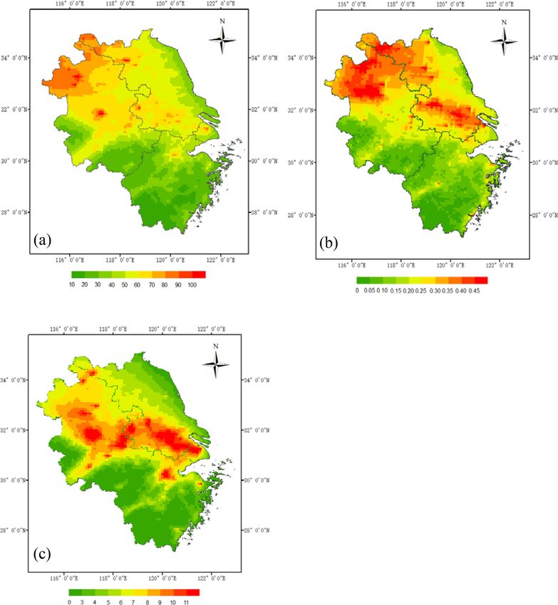
Y. Zhang et al.: Air quality and health benefits from ultra-low emission control policy                                                                                                           6415

Table 1. The air pollutant emissions by sector for cases 1–5 in the YRD (unit: Gg).

  Case                     Power                               Industry                            Residential                       Transportation                             Total
                 SO2        NOx           PM          SO2          NOx            PM         SO2        NOx          PM       SO2          NOx          PM           SO2          NOx            PM
  Case 1       606.8       863.4       376.2       1305.5       1294.6       1817.9        133.5       326.6      787.5       62.0      1847.1        105.9       2107.8       4331.7       3087.4
  Case 2       179.4       245.5        45.1       1305.5       1294.6       1817.9        133.5       326.6      787.5       62.0      1847.1        105.9       1680.5       3713.8       2756.4
  Case 3        56.0       110.0         8.8       1305.5       1294.6       1817.9        133.5       326.6      787.5       62.0      1847.1        105.9       1557.0       3578.4       2720.0
  Case 4        56.0       110.0         8.8        249.4        426.8        539.6        133.5       326.6      787.5       62.0      1847.1        105.9        500.9       2710.6       1441.7
  Case 5         0.0         0.0         0.0       1305.5       1294.6       1817.9        133.5       326.6      787.5       62.0      1847.1        105.9       1501.0       3468.4       2711.2
 Note that for case 1, the emissions of coal-fired power sector were estimated based on the emission factor method without CEMS data. For case 2, the emissions of coal-fired power sector were
 estimated based on the improved method by Y. Zhang et al. (2019), with CEMS data incorporated. For case 3, all the coal-fired power plants in the YRD region were assumed to meet the
 requirement of the ultra-low emission policy. For case 4, all the coal-fired power plants and certain industrial sources including boilers, cement, and iron and steel factories in the YRD region were
 assumed to meet the requirement of the ultra-low emission policy. For case 5, the emissions of all coal-fired power plants were set at zero.

CEMSs, case 3 assumed that only power plants would meet                                                 Compared to another widely used model Global Exposure
the requirement of the ultra-low emission policy, while case 4                                          Mortality Model (GEMM; Burnett et al., 2018), IER was ex-
assumed both power plants and selected industrial sources                                               pected to provide relatively conservative estimates for China
including boilers, cement, and iron and steel factories would                                           (Yang et al., 2021). The number of attributable deaths and
meet the requirement. As summarized in Table S2 in the Sup-                                             years of life lost (YLL) caused by long-term PM2.5 exposure
plement, the ultra-low emission limits for the flue gas con-                                            for selected emission cases were calculated for various dis-
centrations were obtained from the most recent national or                                              eases in this study. In particular, YLL represents the years of
local standards by sector (Yang et al., 2021). The model per-                                           life lost because of premature death from a particular cause
formances were compared with the base case to quantify the                                              or disease. As the number of deaths alone could not provide
air quality improvements that result from the policy. Case 5                                            a comprehensive picture of the burden that deaths impose on
removed all the emissions from the power sector and thus                                                the population, we calculated YLL caused by PM2.5 expo-
helped to specify the contribution of the power sector to air                                           sure to help describe the extent to which the lives of peo-
pollution in the YRD region.                                                                            ple exposed to air pollution were cut short. We considered
   The air pollutant emissions for all the cases are summa-                                             the four adult diseases of the GBD study, including ischemic
rized by sector in Table 1. With the CEMS data for the power                                            heart disease (IHD), stroke (STK, including ischemic and
sector incorporated, the total emissions of SO2 , NOX , and                                             hemorrhagic stroke), lung cancer (LC), and chronic obstruc-
PM for the YRD region in case 2 were estimated as 427,                                                  tive pulmonary disease (COPD), as well as acute lower res-
618, and 331 Gg smaller than those in case 1, with relative                                             piratory infection (LRI), which is a common disease among
reductions of 20 %, 14 %, and 11 %, respectively. Benefit-                                              young children.
ing from the implementation of the ultra-low emission policy                                               The health risks in the different emission cases were es-
in the coal-fired power sector, the total emissions of anthro-                                          timated following Gao et al. (2018) with the updated infor-
pogenic SO2 , NOX , and PM in case 3 would further decline                                              mation for 2015. First, the relative risk (RR) for each disease
123, 135, and 36 Gg compared to case 2, respectively. The                                               was calculated using Eq. (1):
analogous numbers for case 4 were 1180, 1003, and 1315 Gg,
and the reduction rates compared to case 2 were 70 %, 27 %,                                             RRi,j,k (Cl) =
and 48 % for SO2 , NOX and PM, respectively. The imple-
mentation of the ultra-low emission policy for both power                                                                                     γi,j,k
                                                                                                         (
                                                                                                             1 + ∂i,j,k 1 − e−βi,j,k (Cl−C0 )          , Cl ≥ C0
and industrial sectors would significantly reduce the primary                                                                                                                                        (1)
pollutant emissions for the YRD region. In case 5 where the                                                  1,                                          Cl < C0 ;
emissions from the power sector were set as zero, the total
emissions of SO2 , NOX , and PM were estimated to decrease                                              where i, j , and k represent the age, gender, and disease type,
by 11 %, 7 %, and 2 %, respectively, compared to case 2.                                                respectively; “Cl” is the annual average PM2.5 concentration
                                                                                                        simulated with WRF-CMAQ (the average of January, April,
2.3     Health effect analysis                                                                          July, and October in this work); C0 is the counterfactual con-
                                                                                                        centration; and ∂, β, and γ are the parameters that describe
We applied the IER model of the Global Burden of Disease                                                the IER functions, as reported by Cohen et al. (2017).
(GBD) study 2015 (Cohen et al., 2017) and quantified the                                                   Secondly, the population attributable fractions (PAFs)
impact of emission control policy on the human health risk                                              were calculated with RR following Eq. (2) by disease, age,
due to long-term exposure of PM2.5 in the YRD region. The                                               and gender subgroup:
model has been well developed and widely applied in quan-
tifying the impact of air pollution control policies on health                                                             RRi,j,k (Cl) − 1
                                                                                                        PAFi,j,k =                          .                                                        (2)
burden (Li et al., 2019; Yue et al., 2020; Zheng et al., 2019).                                                             RRi,j,k (Cl)

https://doi.org/10.5194/acp-21-6411-2021                                                                                           Atmos. Chem. Phys., 21, 6411–6430, 2021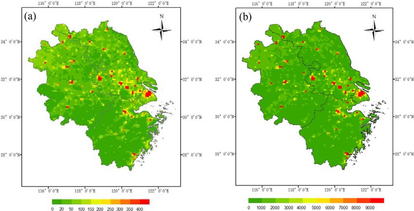
6416                                   Y. Zhang et al.: Air quality and health benefits from ultra-low emission control policy

Moreover, the mortality attributable to PM2.5 exposure              test the improvement of emission estimates. Because of the
(1M) was calculated using Eq. (2), where y0 is the current          combined influences of regional transport and chemical reac-
age–gender-specific mortality rate, and “Pop” represents the        tions of air pollutants in the atmosphere, nonlinear relation-
exposed population in the age–gender-specific group in grid         ships were found between the changes of primary emissions
cell l:                                                             and ambient concentrations of air pollutants. Compared to
                                                                    case 1, the simulated annual average concentrations of SO2 ,
1Mi,j,k,l = PAFi,j,k,l × y0i,j,k,l × Popi,j,l .             (3)     NO2 , and PM2.5 in the YRD region were 10 %, 7 %, and
                                                                    6 % lower, respectively, in case 2, while that of O3 was 7 %
The population data of the four provinces and cities in             higher, due to combined effects of emissions of volatile or-
the YRD region were obtained from statistical yearbooks             ganic compounds (VOCs) and NOX precursors (Gao et al.,
(AHBS, 2016; JSBS, 2016; SHBS, 2016; ZJBS, 2016), and               2005; Yang et al., 2012). Previous studies have shown that
the gender distribution by province is shown in Table S3            O3 formation in most of the YRD region is under the “VOCs-
in the Supplement. As the high-resolution spatial pattern           limited” regime, i.e., the generation and removal of O3 is
of age structure was unavailable, we assumed the same               more sensitive to VOCs and would be inhibited with high
age structure for all the model grids according to Gao et           NOX concentrations in the atmosphere (Zhang et al., 2008;
al. (2018). The baseline age–gender–disease-specific mortal-        Liu et al., 2010; Wang et al., 2010; Xing et al., 2011). There-
ity rates for the five diseases in China for 2015 were obtained     fore, the simulated reduced NO2 concentrations from greater
from the Global Health Data Exchange database (GHDx,                NOX emission control could elevate the O3 concentration.
https://vizhub.healthdata.org, last access: 19 April 2021), as         The model performance was evaluated with available
shown in Table S4 in the Supplement, and those by province          ground observation. The hourly concentrations were ob-
were calculated based on the provincial proportions in Xie et       served at 230 state-operated air quality monitoring stations
al. (2016). The national population with the spatial resolution     within YRD, and the averages of hourly concentrations of
at 1 km× 1 km in 2015 was provided by the LandScan global           those sites were compared with the simulations in cases 1 and
demographic dynamic analysis database developed by Oak              2, as summarized in Table 2. Similar model performances
Ridge National Laboratory (ORNL) of the US Department               were found for the two emission cases, with overestima-
of Energy. As shown in Fig. S1 in the Supplement, the pop-          tion of SO2 , NO2 , and PM2.5 as well as underestimation of
ulation densities in the YRD region are larger in Shanghai,         O3 . The NMEs between the simulated and observed SO2 ,
southern Jiangsu, and northern Zhejiang.                            O3 , and PM2.5 concentrations were all smaller than 50 % for
   Finally, the year of life lost (YLL) due to PM2.5 exposure       both cases and slightly worse simulation performances were
was calculated from the number of deaths multiplied by a            found in July compared to the other 3 months. In particular,
standard life expectancy at the age at which death occurs, as       the correlation coefficients (R) between the simulated and
shown in Eq. (4), where N represents the number of deaths in        observed SO2 in July were only 0.17 and 0.14 for cases 1 and
each age–gender-specific group, and L reflects the remaining        2, respectively, and the NMEs between the simulated and ob-
life expectancy of the group:                                       served NO2 were larger than 100 %. In addition, greater over-
         X                                                          estimation of SO2 and PM2.5 by the model was found in July
YLL =           N × Li,j .
             i,j i,j
                                                             (4)    compared to other months, likely attributable to the bias of
                                                                    WRF modeling. On the one hand, the simulated WS10 in the
The remaining life expectancies by age data were obtained           YRD region in July (2.67 m s−1 ) was slightly lower than the
from the life tables from the World Health Organization             observation (2.75 m s−1 ). The underestimation in wind speed
(WHO, https://www.who.int, last access: 19 April 2021), as          could weaken the horizontal diffusion and lead to overesti-
summarized in Table S5 in the Supplement. The life ex-              mation in air pollutant concentrations. Compared with the re-
pectancies at birth of Chinese males and females in 2015            sults from the European Centre for Medium-Range Weather
were 74.8 and 77.7 years, respectively.                             Forecasts (ECMWF, https://apps.ecmwf.int/datasets, last ac-
                                                                    cess: 19 April 2021), on the other hand, the simulated bound-
                                                                    ary layer height (BLH) was lower in WRF for all months.
3     Results and discussion
                                                                    The NMBs of the WRF and ECMWF BLH in January, April,
3.1     Evaluation of emission estimates with air quality           and October were around −15 %, while that in July reached
        simulation                                                  −24 %. The lower BLH would limit the vertical convection
                                                                    and diffusion of pollutants and thereby increase the surface
3.1.1    Model performances with and without CEMS                   concentrations of air pollutants. Similar to previous studies
         data                                                       (An et al., 2013; Liao et al., 2015; Tang et al., 2015; Gao
                                                                    et al., 2016; Wang et al., 2016; Zhou et al., 2017), underes-
Air quality simulations based on emission inventories with          timation of O3 was commonly found. The NMBs between
and without incorporation of CEMS data for the coal-fired           the simulation and observation for the two cases ranged from
power sector (cases 1 and 2, respectively) were conducted to        −34.5 % to −6.4 % and NMEs from 23.1 % to 37.1 %, re-

Atmos. Chem. Phys., 21, 6411–6430, 2021                                              https://doi.org/10.5194/acp-21-6411-2021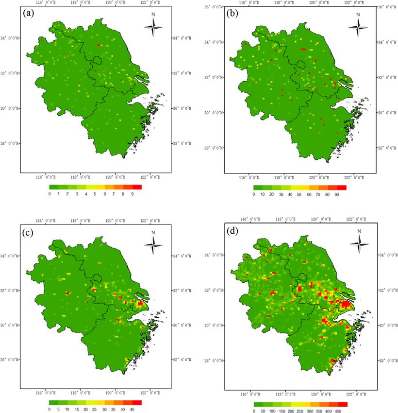
Y. Zhang et al.: Air quality and health benefits from ultra-low emission control policy                                                        6417

Table 2. Comparison of the observed and simulated hourly SO2 , NO2 , O3 , and PM2.5 concentrations by month for cases 1 and 2 in the YRD
region. In total, 230 state-operated observation sites were included in the comparison.

                            Pollutant                       R                       NMB (%)                       NME (%)
                                                  Case 1            Case 2      Case 1        Case 2        Case 1          Case 2
                            SO2          Jan         0.72               0.89↑    11.44      0.52↑∗∗          26.83         24.22↑
                                         Apr         0.36               0.45↑   −18.45      −22.62           31.65          34.81
                                         Jul         0.17                0.14    36.84   15.72↑∗∗∗           58.69         48.44↑
                                         Oct         0.59                0.57    14.59    1.15↑∗∗∗           32.49        29.22↑∗
                            NO2          Jan         0.72               0.73↑    42.74     34.92↑∗           44.25         37.88↑
                                         Apr         0.64               0.69↑    69.24   48.72↑∗∗∗           70.24       51.81↑∗ *
                                         Jul         0.71                0.71   145.42    131.65↑∗          145.42       131.65↑∗
                                         Oct         0.70                0.69    58.15     47.73↑∗           58.86        49.41↑∗
                            O3           Jan         0.74               0.75↑   −16.90    −6.40↑∗∗           30.53          28.60↑
                                         Apr         0.78                0.67   −14.88      −9.89↑           23.14           27.48
                                         Jul         0.78               0.79↑   −34.49     −28.46↑           37.11          32.77↑
                                         Oct         0.80                0.78   −30.37     −28.28↑           34.32          33.60↑
                            PM2.5        Jan         0.89               0.90↑   −0.28          1.63          16.27         15.21↑
                                         Apr         0.76                0.76    9.94      2.57↑∗∗           21.30         19.26↑
                                         Jul         0.64                0.63   30.44    24.08↑∗∗∗           37.66        34.29↑∗
                                         Oct         0.75                0.75    5.40       −11.80           23.34          22.28
                          Note that the arrows indicate that the simulation values in case 2 were improved compared to case 1. The ∗ ,
                          ∗∗ , and ∗∗∗ symbols indicate the improvements are statistically significant with confidence levels of 90 %,
                          95 %, and 99 %, respectively. The R , NMB, and NME were calculated using the following equations (where
                          P , O , (P ), and (O) represent the simulation, observation, averaged simulation, and averaged observation
                                                           Pn (P −O )                       nP
                                                                                                P −Oi
                          values, respectively): NMB =       Pn i
                                                            i=1      i
                                                                       × 100 %; NME =        Pn i
                                                                                            i=1       × 100 %;
                                    Pn                        i=1 Oi                          i=1 Oi
                                     (Pi −P )(Oi −O)
                          R = qP i=1                                .
                                n        2 Pn                   2
                                   i=1 (Pi −P )   i=1 (Oi −O)

spectively. The underestimation in O3 likely resulted from                           al., 1996; He et al., 2017) was further applied to test the
bias in the estimation of precursor emissions. Suggested by                          significance of the improvements of case 2 over case 1. (A
the positive NMBs of NO2 modeling in Table 2, the NOX                                significant difference is demonstrated if the confidence inter-
emissions were expected to be overestimated in the two                               vals of given statistical indices sampled from the two cases
cases, even for case 2 with the CEMS data incorporated                               do not overlap.) As can be seen in Table 2, the modeling
(which reflect the emission control benefits in recent years, as                     performances of the concerned species in case 2 were im-
discussed in Y. Zhang et al., 2019). In addition, underestima-                       proved significantly in most instances compared to case 1.
tion of VOC emissions is likely due to incomplete accounting                         For example, the improvement of NMB for the SO2 simula-
of emission sources, particularly for uncontrolled or fugitive                       tion was significant at the 99 % confidence level for July and
leakage (Zhao et al., 2017). As most of YRD was identified                           October and 95 % for January. The improvement of NMB
as a VOC-limited region for O3 formation (Wang et al., 2019;                         and NME for NO2 was significant at confidence levels of
Yang et al., 2021), the overestimation of NOX and underes-                           99 % and 95 %, respectively, for April. The improvement of
timation of VOCs could contribute to the underestimation in                          NMB for O3 was significant at the 95 % confidence level for
O3 concentrations with air quality modeling. The simulations                         January and that of PM2.5 at 95 % for April and 99 % for
of both cases captured well the temporal variations of PM2.5                         July. The statistical test confirms that incorporation of online
concentrations, with the R between the observed and simu-                            monitoring data in the emission inventory can improve the
lated concentrations around 0.9.                                                     regional air quality modeling for the YRD region. Besides
   In general, better modeling performance in the YRD re-                            the emission data, it should also be noted that the changes in
gion was found in case 2 than case 1. The NMBs between the                           model schemes would affect the model performance. For ex-
simulated and observed concentrations of SO2 , NO2 , O3 , and                        ample, the newer version of CMAQ incorporated the chem-
PM2.5 for the whole simulation period were −3.1 %, 56.3 %,                           istry schemes of bromine and iodine and was expected to in-
−19.5 %, and −1.4 % for case 2, which were smaller in ab-                            fluence the O3 simulation importantly. According to our re-
solute value than those for case 1 at 8.2 %, 68.9 %, −24.6 %,                        cent test in the YRD region (Lu et al., 2020), the impact of
and 7.6 %, respectively. The bootstrap sampling (Gleser et                           CMAQ version on the simulation of difference species was

https://doi.org/10.5194/acp-21-6411-2021                                                                   Atmos. Chem. Phys., 21, 6411–6430, 2021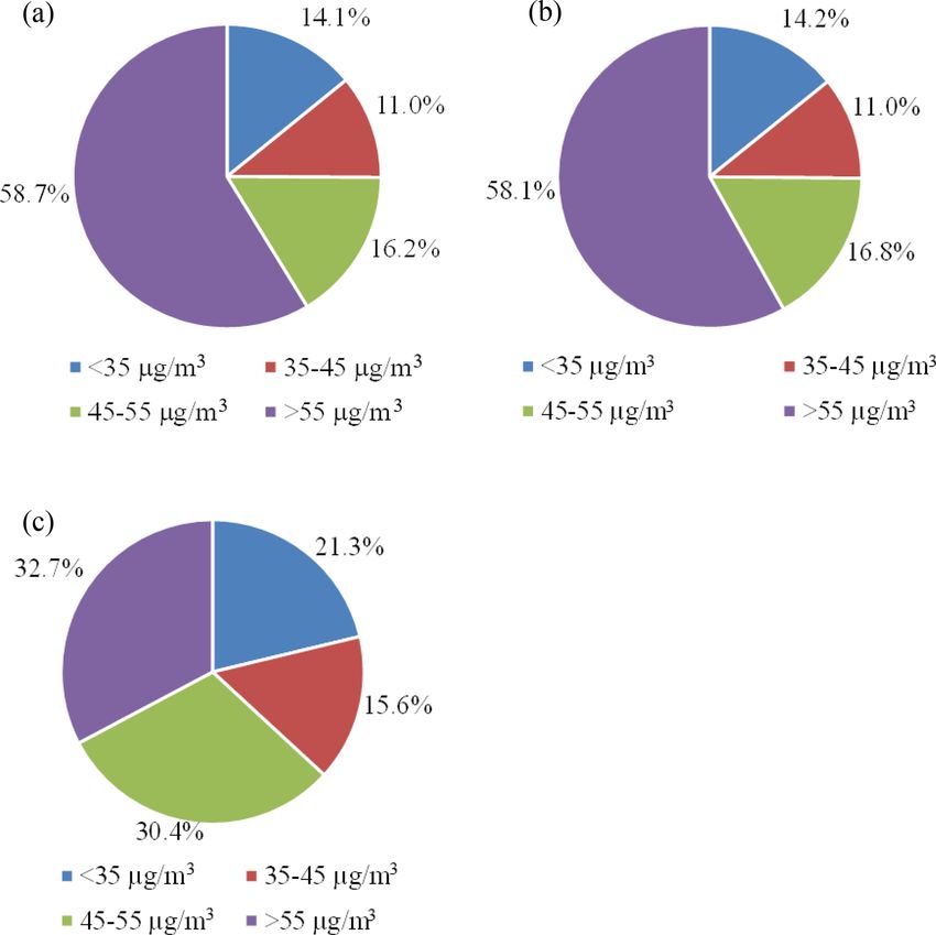
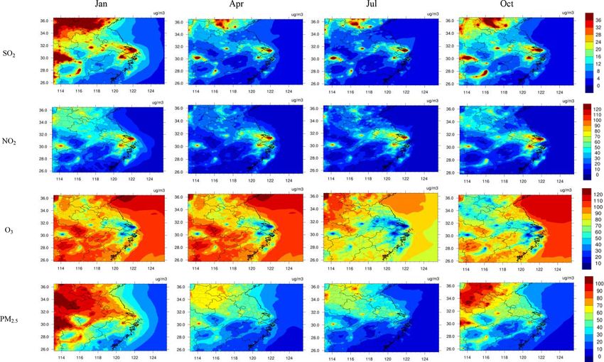
6418                                   Y. Zhang et al.: Air quality and health benefits from ultra-low emission control policy

Figure 2. The spatial distributions of the simulated monthly SO2 , NO2 , O3 , and PM2.5 concentrations for case 2 in D2 (unit: µg m−3 ).

inconclusive, implying the necessity of further intercompari-            dition, O3 concentrations could remain relatively high after
son and evaluation studies for the region.                               transport from urban to the suburban areas due to relatively
   Figure 2 illustrates the spatial patterns of the simulated            small emissions of NOX in the latter.
monthly SO2 , NO2 , O3 and PM2.5 concentrations for case 2.
For a given species, similar patterns were found for differ-             3.1.2   Benefits of the ultra-low emission controls on air
ent months. In general, the simulated concentrations of SO2 ,                    quality
NO2 , and PM2.5 were larger in central and northern Anhui,
southern Jiangsu, Shanghai, and coastal areas in Zhejiang,               Table 3 summarizes the absolute and relative changes of the
where large power and industrial plants are concentrated, as             simulated monthly concentrations of the concerned air pol-
shown in Fig. S2 in the Supplement. In the highly populated              lutants in cases 3–5 compared to the base case (case 2). The
cities (Shanghai, Nanjing, Hangzhou, and Hefei; see their lo-            average contributions of the power sector to the total am-
cations in Fig. 1), the simulated concentrations of pollutants           bient concentrations of SO2 , NO2 , and PM2.5 for the four
were significantly larger than their surrounding areas. For ex-          simulated months are estimated at 10.0 %, 4.7 %, and 2.3 %,
ample, the simulated SO2 , NO2 , and PM2.5 concentrations in             respectively, based on comparison of cases 2 and 5. The con-
Nanjing were 1.4, 1.3, and 1.2 times of those in its nearby              tributions to the concentrations were close to those of emis-
cities. The analogous numbers for Hangzhou were 2.5, 1.5,                sions at 10.7 %, 6.6 %, and 1.6 % for the three species (as
and 1.3. In contrast, the simulated O3 concentrations were               indicated in Table 1), respectively. The larger power sec-
smaller in urban areas and larger in suburban ones. For in-              tor contribution to the ambient PM2.5 concentrations than to
stance, the simulated O3 in Nanjing, Shanghai, Hefei, and                primary PM emissions reflects high emissions of precursors
Hangzhou were 0.7, 0.4, 0.6, and 0.6 times of those in their             of secondary sulfate and nitrate aerosols. In general, limited
surrounding areas, respectively. The spatial distributions of            contributions from the power sector were found for all con-
the simulated NO2 and O3 concentrations in Fig. 2 also in-               cerned species except SO2 , which is attributed to the gradu-
dicated that O3 concentrations were less in the regions with             ally improved controls in the sector. The further implemen-
higher NO2 concentrations, such as the megacity of Shang-                tation of the ultra-low emission policy in the sector, there-
hai. The simulated high concentrations of NO2 in urban areas             fore, is expected to result in limited additional benefits for
promotes titration of O3 , reducing its concentrations. In ad-           air quality. As shown in Table 3, the absolute changes of the

Atmos. Chem. Phys., 21, 6411–6430, 2021                                                     https://doi.org/10.5194/acp-21-6411-2021
Y. Zhang et al.: Air quality and health benefits from ultra-low emission control policy 6419
Table 3. The relative (%) and absolute changes (µg m−3 , in parentheses) of the simulated monthly pollutant concentrations in different cases
relative to case 2 in the YRD region.
Pollutant (case 3 − case 2) / case 2 (case 4 − case 2) / case 2 (case 5 − case 2) / case 2
Jan Apr Jul Oct Jan Apr Jul Oct Jan Apr Jul Oct
SO2 −2.7 −4.8 −6.1 −4.3 −32.9 −57.3 −64.1 −55.1 −4.3 −11.4 −12.1 −12.1
(−0.2) (−0.2) (−0.1) (−0.2) (−2.0) (−1.8) (−1.5) (−2.4) (−0.3) (−0.4) (−0.3) (−0.5)
NO2 −2.0 −2.9 −2.0 −2.5 −16.4 −21.9 −17.1 −22.8 −2.6 −5.9 −4.1 −6.2
(−0.4) (−0.4) (−0.3) (−0.4) (−3.2) (−3.0) (−2.5) (−3.7) (−0.5) (−0.8) (−0.6) (−1.0)
O3 1.7 2.2 0.8 2.2 10.4 9.7 2.6 14.0 −2.0 2.7 −1.6 4.5
(0.4) (0.9) (0.3) (0.8) (2.6) (4.1) (0.8) (4.8) (−0.5) (1.2) (−0.5) (1.5)
PM2.5 −0.1 −0.5 −1.3 −0.5 −6.2 −14.6 −21.6 −14.3 −1.7 −2.4 −4.3 −0.9
(−0.1) (−0.2) (−0.4) (−0.2) (−4.6) (−6.0) (−6.5) (−6.3) (−1.3) (−1.0) (−1.3) (−0.4)
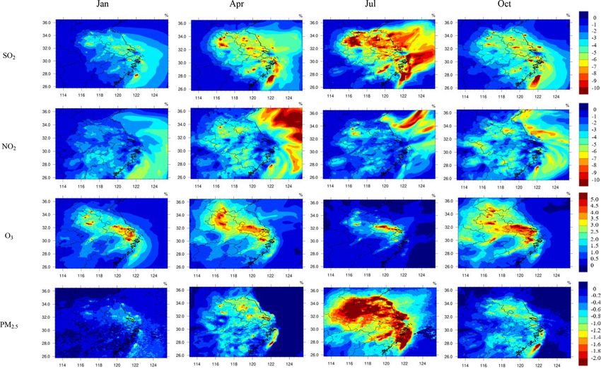
Figure 3. The spatial distributions of the relative changes (%) in the simulated monthly SO2 , NO2 , O3 , and PM2.5 concentrations between
cases 2 and 3 in D2 ((case 3 − case 2) / case 2).
simulated SO2 , NO2 , O3 , and PM2.5 concentrations in case 3 low emission policy was broadened from the power sector
compared to case 2 were all smaller than 1 µg m−3 for the to the industrial sector (case 4), which is attributed to the
4 months. Larger changes were found for primary pollutants dominant role of industry in air pollutant emissions in the
(SO2 and NO2 ) than for those of secondary ones (O3 and YRD region (Table 1). The simulated monthly concentra-
PM2.5 ): the simulated monthly concentrations of SO2 and tions of SO2 , NO2 and PM2.5 were 1.5–2.0, 2.5–3.7, and
NO2 were 2.7 %–6.1 % and 2.0 %–2.9 % lower, while PM2.5 4.6–6.5 µg m−3 lower compared to the base case, respec-
was only 0.1 %–1.3 % lower and O3 0.8 %–2.2 % higher, re- tively, or reduction rates of 32.9 %–64.1 %, 16.4 %–22.8 %,
spectively. Much larger benefits were found when the ultra- and 6.2 %–21.6 %. In contrast, the simulated O3 concentra-
https://doi.org/10.5194/acp-21-6411-2021 Atmos. Chem. Phys., 21, 6411–6430, 20216420 Y. Zhang et al.: Air quality and health benefits from ultra-low emission control policy Figure 4. The spatial distributions of the relative changes (%) in the simulated monthly SO2 , NO2 , O3 , and PM2.5 concentrations between cases 2 and 4 in D2 ((case 4 − case 2) / case 2). tion was 0.8–4.8 µg m−3 higher, with growth rates ranging over, the relatively low concentrations in summer also con- 2.6 %–14.0 %. As mentioned earlier, the YRD was identi- tributed to the largest percentage changes in SO2 and PM2.5 fied as a VOC-limited region, and reducing NOX emissions simulation for the season. without any VOC controls would enhance O3 concentrations. Figures 3 and 4 illustrate the spatial distributions of the rel- Currently, CEMSs do not report VOC concentrations in the ative changes of simulated pollutant concentrations in cases 3 flue gas, and the ultra-low emission policy does not include a and 4 compared to case 2, respectively. As shown in Fig. 3, VOC limit, either. In order to alleviate regional air pollution the overall changes across the region due to ultra-low emis- including O3 , coordinated controls of NOX and VOC emis- sion controls in the power sector only were less than 10 % sions are urgently required. These would include measures for primary pollutants SO2 and NO2 and 5 % for secondary to reduce large sources of VOCs, notably in industries other pollutants PM2.5 and O3 . Larger changes in simulated SO2 than the power industry such as the chemicals and refining concentrations were found in central and northern Anhui as industry and in solvent use (Zhao et al., 2017). well as central and southern Jiangsu, with relatively concen- The relative changes in the simulated pollutant concen- trated distribution of coal-fired power plants. The changes of trations varied by month, due to the combined influences simulated SO2 and NO2 in Shanghai were tiny, due to few re- of meteorology and secondary chemistry, and larger relative maining power plants subject to the ultra-low emission pol- changes were found for SO2 and PM2.5 in summer. As shown icy and thus few emission reductions. Compared to case 2, in Table 3, for example, the average simulated PM2.5 concen- the SO2 and NOX emissions in case 3 were estimated to be trations in July were 0.4 and 6.5 µg m−3 lower, respectively, 2.2 % and 0.8 % lower, respectively, for Shanghai, i.e., much under cases 3 and 4 compared to case 2, with the larger re- smaller than for other provinces (6.1 % and 2.5 % for An- duction than other 3 months. This could result partly from hui, 9.5 % and 4.4 % for Jiangsu, and 5.5 % and 2.7 % for the faster response of ambient concentrations to the changed Zhejiang). The results suggest that the potential of emission emissions of air pollutants with shorter lifetimes in summer. reduction and air quality improvement is limited from imple- The formation of secondary pollutants like PM2.5 would be mentation of more stringent control measures in the power enhanced in summer, with more oxidative atmospheric con- sector alone, particularly in highly developed cities where ditions under high temperature and strong sunlight. More- Atmos. Chem. Phys., 21, 6411–6430, 2021 https://doi.org/10.5194/acp-21-6411-2021
Y. Zhang et al.: Air quality and health benefits from ultra-low emission control policy                                                 6421

Figure 5. The spatial distributions of the annual PM2.5 concentrations (average of January, April, July, and October) for case 2 (a) and the
reduced annual PM2.5 concentrations for cases 3 (b) and 4 (c) in the YRD region (unit: µg m−3 ). Note the different color ranges in the panels
for easier visualization.

air pollution controls have already reached a relatively high            little regional disparity in the changed ambient SO2 levels.
level.                                                                   Compared to other areas, the relatively less reduction in the
   In case 4, where both power plants and selected industrial            simulated NO2 in central YRD resulted in significant en-
sources meet the ultra-low emission requirement, the aver-               hancement of O3 concentrations (note that much more re-
age reduction rates of simulated SO2 and NO2 concentra-                  duction in NO2 resulted in similar enhancement of O3 in
tions compared to case 2 were above 40 % and 25 %, respec-               southern Anhui for October). The comparison implies that
tively, for the whole region, and the changes of secondary               the O3 formation in central YRD was more sensitive to NOX
pollutants O3 and PM2.5 were also significantly larger than              emission abatement than other VOC-limited regions in the
those of case 3 in most of the region. The relative changes of           YRD. The result suggests a particularly great challenge of O3
SO2 were found to be more significant than other species,                pollution control in central YRD, and more efforts on VOC
as the SO2 concentrations are greatly affected by primary                emission abatement would be required for those developed
emissions. Due to the large number and wide distribution of              areas.
industrial plants throughout the YRD, moreover, there was

https://doi.org/10.5194/acp-21-6411-2021                                                    Atmos. Chem. Phys., 21, 6411–6430, 2021
6422                                 Y. Zhang et al.: Air quality and health benefits from ultra-low emission control policy

                                                                    21 % in case 4, from 11 % to 16 %, and from 16 % to 30 %,
                                                                    respectively (note that 35 µg m−3 is the annual PM2.5 con-
                                                                    centration limit in the current National Ambient Air Qual-
                                                                    ity Standard for China). Accordingly, the fraction exposed
                                                                    to PM2.5 concentrations larger than 55 µg m−3 declined from
                                                                    59 % to 33 %. The implementation of ultra-low emission pol-
                                                                    icy on both power plants and industry sources thus proved
                                                                    an effective way in limiting the population exposed to high
                                                                    PM2.5 levels.

                                                                    3.2.2   Human health risk with base case emissions

                                                                    The mortality and YLL caused by atmospheric PM2.5 ex-
                                                                    posure with the base case emissions (case 2) in the YRD
                                                                    region are shown in Table 4. The values in brackets repre-
                                                                    sent the 95 % confidence interval (CI) attributed to the un-
                                                                    certainty of IER curves (i.e., uncertainties from other sources
                                                                    were excluded in the 95 % CI estimation such as air qual-
                                                                    ity model mechanisms, emission inventories, and population
                                                                    data). With the base case emissions, the NMB of the simu-
                                                                    lated and observed annual PM2.5 concentrations (based on
Figure 6. The population fractions exposed to different levels of   the four representative months) was calculated at −1.4 %
PM2.5 in the YRD region for cases 2 (a), 3 (b), and 4 (c).
                                                                    for the YRD region. Therefore, the influence of the bi-
                                                                    ases between the simulations and observations on the esti-
                                                                    mated health risks was negligible and thus not considered in
3.2     Evaluation of health benefits                               this study. The total attributable deaths due to all diseases
                                                                    caused by PM2.5 exposure in the YRD region were esti-
3.2.1    PM2.5 exposures in the YRD region                          mated at 194 000 (114 000–282 000), with STK, IHD, and
                                                                    COPD causing the most deaths, accounting for 29 %, 32 %,
Figure 5 illustrates the spatial distributions of PM2.5 con-        and 22 % of the total, respectively. With larger populations
centrations for the base case (case 2) and the differences          in Anhui and Jiangsu (32 % and 37 % of the regional total,
of cases 3 and 4 compared to the base case. The reduc-              respectively), more deaths caused by PM2.5 exposure were
tion of PM2.5 concentrations from the implementation of the         found in these two provinces, at 34 % and 41 % of the total
ultra-low emission policy in the power sector was less than         deaths, respectively. Among all the diseases, STK was found
1 µg m−3 over the YRD region (Fig. 5b). Larger reductions           to cause the largest number of mortalities (19 600) in Anhui
(above 0.4 µg m−3 ) were found in northern Anhui and north-         with PM2.5 exposure, IHD in Jiangsu (31 300), and COPD
ern and southern Jiangsu provinces, as those regions are the        in Shanghai (4400) and Zhejiang (10 800). The total YLL
energy base of eastern China, with abundant coal mines and          caused by PM2.5 exposure in the YRD region was 5.11 mil-
power plants with large installed capacities. With the policy       lion years (3.16–7.18 million years). More YLL caused by
expanded to certain industrial sectors, the simulated average       PM2.5 exposure was found in Anhui and Jiangsu, account-
PM2.5 concentrations were 5.8 µg m−3 lower for the whole            ing for 34 % and 37 % of the total in the YRD region, re-
region (Fig. 5c). In particular, the difference was greater than    spectively. YLL values caused by COPD were the largest in
10 µg m−3 along the Yangtze River, as there are many indus-         all the provinces, with 0.66 million, 0.19 million, 0.56 mil-
trial parks located along the river containing a large number       lion, and 0.47 million years estimate for Anhui, Shanghai,
of big cement, iron and steel, and chemical industry plants.        Jiangsu, and Zhejiang, respectively. The spatial distribution
Stringent emission controls at those plants would result in         of attributable deaths and YLL caused by PM2.5 exposure
significant benefits in air quality for local residents.            was basically consistent with that of population in the YRD
   We further calculated the fractions of the population with       region, with correlation coefficients of 0.94 and 0.96, respec-
different annual average PM2.5 exposure levels in cases 2–4,        tively. As shown in Fig. 7, higher health risks attributed to
as shown in Fig. 6. Compared to case 2, slight differences          PM2.5 pollution in the base case (case 2) were commonly
in the population distribution by exposure level were found         found in the areas with larger population densities, includ-
in case 3, while the differences were much more significant         ing the areas along the Yangtze River, central Shanghai and
in case 4. The population fractions exposed to the average          some urban areas in Anhui. We further compared the pop-
annual concentrations of PM2.5 smaller than 35, 35–45, and          ulation deaths attributable to PM2.5 exposure calculated in
45–55 µg m−3 were estimated to grow from 14 % in case 2 to          this study with the reported total deaths in provincial sta-

Atmos. Chem. Phys., 21, 6411–6430, 2021                                              https://doi.org/10.5194/acp-21-6411-2021
Y. Zhang et al.: Air quality and health benefits from ultra-low emission control policy 6423
Table 4. The estimated mortality and YLL attributable to PM2.5 exposures in case 2 over the YRD region.
STK IHD COPD LC LRI Total
Deaths (× 103 persons)
Anhui 19.6 (10.7–29.0) 19.1 (11.0–29.8) 15.2 (9.8–21.0) 8.0 (5.5–10.3) 3.1 (2.4–3.8) 65.0 (39.4–93.9)
Shanghai 4.3 (2.3–6.5) 4.2 (2.4–6.6) 4.4 (2.7–6.1) 2.6 (1.7–3.3) 0.8 (0.6–1.0) 16.3 (9.8–23.4)
Jiangsu 23.6 (12.7–35.0) 31.3 (17.8–48.8) 12.8 (8.1–17.7) 8.1 (5.5–10.5) 3.7 (2.8–4.5) 79.5 (46.8–116.5)
Zhejiang 8.7 (4.2–13.4) 6.8 (3.6–10.4) 10.8 (6.2–15.4) 5.0 (3.1–6.9) 1.6 (1.1–2.0) 32.9 (18.2–48.2)
YRD 56.2 (29.9–83.8) 61.4 (34.7–95.5) 43.3 (26.8–60.2) 23.6 (15.8–31.0) 9.2 (7.0–11.3) 193.8 (114.2–281.9)
YLL (× 104 years)
Anhui 30.1 (16.6–44.0) 29.6 (17.3–45.6) 66.0 (42.3–91.1) 34.5 (23.7–44.4) 13.6 (10.4–16.4) 173.7 (110.3–241.5)
Shanghai 6.7 (3.6–9.8) 6.5 (3.8–10.0) 19.0 (11.9–26.2) 11.0 (7.4–14.4) 3.5 (2.7–4.3) 46.7 (29.4–64.8)
Jiangsu 36.2 (19.7–53.1) 48.6 (28.0–74.7) 55.6 (35.0–76.7) 35.0 (23.6–45.6) 16.0 (12.3–19.4) 191.4 (118.5–269.5)
Zhejiang 13.3 (6.5–20.5) 10.6 (5.7–16.0) 46.9 (26.7–66.6) 21.8 (13.6–30.0) 6.8 (4.8–8.9) 99.4 (57.2–141.9)
YRD 86.3 (46.3–127.4) 95.3 (54.7–146.4) 187.4 (115.9–260.6) 102.3 (68.3–134.4) 40.0 (30.1–48.9) 511.3 (315.5–717.7)
Figure 7. The spatial distributions of the mortality (a) and YLL (b) attributable to PM2.5 exposure in case 2 at a horizontal resolution of
9 km.
tistical yearbooks (AHBS, 2016; JSBS, 2016; SHBS, 2016; ities between them due to different estimation methods and
ZJBS, 2016) and found that the deaths caused by PM2.5 ex- health endpoints selected. Figure 8 compares the estimates
posure accounted for 18 %, 14 %, 15 %, and 11 % of the total of premature deaths caused by PM2.5 exposure in the YRD
deaths in Anhui, Jiangsu, Shanghai, and Zhejiang, respec- region in this and previous studies. Relatively close results
tively, for 2015. The numbers were larger than the estimate are found between studies for the same regions and periods.
(6.9 %) by Maji et al. (2018), which focused on 161 cities For example, Hu et al. (2017) and Liu et al. (2016) esti-
in China. As one of the most developed and industrialized mated that the premature deaths of adults (> 30 years old)
regions in China, the YRD suffered higher PM2.5 pollution due to PM2.5 exposure were 223 000 and 245 000, respec-
level than the national average, leading to the larger fraction tively, in 2013 in the YRD region. However, the health end-
of premature death due to PM2.5 exposure. Moreover, the points in these two studies were not completely consistent.
baseline disease-specific mortality rates applied in this study COPD, LC, IHD, and CEV (cerebrovascular disease) were
(from GHDx) were commonly higher than those in Maji et selected in Hu et al. (2017), while COPD, LC, IHD, and
al. (2018) except for LRI, resulting in the larger estimate of STK were chosen by Liu et al. (2016). The deaths caused
death rates exposed to PM2.5 . by PM2.5 exposure in Shanghai were estimated at 19 000,
Many studies have focused on the human health risks at- 15 000, and 16 000 in Maji et al. (2018), Song et al. (2017),
tributable to air pollution in China, with considerable dispar- and this study, respectively. The IER model and the same
https://doi.org/10.5194/acp-21-6411-2021 Atmos. Chem. Phys., 21, 6411–6430, 2021You can also read