Effects of spatial resolution on WRF v3.8.1 simulated meteorology over the central Himalaya - GMD
←
→
Page content transcription
If your browser does not render page correctly, please read the page content below
Geosci. Model Dev., 14, 1427–1443, 2021
https://doi.org/10.5194/gmd-14-1427-2021
© Author(s) 2021. This work is distributed under
the Creative Commons Attribution 4.0 License.

Effects of spatial resolution on WRF v3.8.1 simulated meteorology
over the central Himalaya
Jaydeep Singh1 , Narendra Singh1 , Narendra Ojha2 , Amit Sharma3 , Andrea Pozzer4,5 , Nadimpally Kiran Kumar6 ,
Kunjukrishnapillai Rajeev6 , Sachin S. Gunthe7 , and V. Rao Kotamarthi8
1 Aryabhatta Research Institute of observational sciencES (ARIES), Nainital, India
2 PhysicalResearch Laboratory, Ahmedabad, India
3 Department of Civil and Infrastructure Engineering, Indian Institute of Technology Jodhpur, Jodhpur, India
4 Department of Atmospheric Chemistry, Max Planck Institute for Chemistry, Mainz, Germany
5 Earth System Physics Section, International Centre for Theoretical Physics, Trieste, Italy
6 Space Physics Laboratory, Vikram Sarabhai Space Centre, Thiruvananthapuram, India
7 EWRE Division, Department of Civil Engineering, Indian Institute of Technology Madras, Chennai, India
8 Environmental Science Division, Argonne National Laboratory, Argonne, Illinois, USA

Correspondence: Narendra Singh (narendra@aries.res.in) and Andrea Pozzer (andrea.pozzer@mpic.de)

Received: 13 January 2020 – Discussion started: 3 March 2020
Revised: 13 January 2021 – Accepted: 1 February 2021 – Published: 15 March 2021

Abstract. The sensitive ecosystem of the central Himalayan       perature (warm bias by 2.8 ◦ C) and underestimates RH
(CH) region, which is experiencing enhanced stress from          (dry bias by 6.4 %) at the surface in d01. Model results
anthropogenic forcing, requires adequate atmospheric ob-         show a significant improvement in d03 (P = 827.6 hPa,
servations and an improved representation of the Himalaya        T = 19.8 ◦ C, RH = 92.3 %), closer to the GVAX observa-
in the models. However, the accuracy of atmospheric mod-         tions (P = 801.4 hPa, T = 19.5 ◦ C, RH = 94.7 %). Interpo-
els remains limited in this region due to highly complex         lating the output from the coarser domains (d01, d02) to the
mountainous topography. This article delineates the effects      altitude of the station reduces the biases in pressure and tem-
of spatial resolution on the modeled meteorology and dy-         perature; however, it suppresses the diurnal variations, high-
namics over the CH by utilizing the Weather Research and         lighting the importance of well-resolved terrain (d03). Tem-
Forecasting (WRF) model extensively evaluated against the        poral variations in near-surface P , T , and RH are also re-
Ganges Valley Aerosol Experiment (GVAX) observations             produced by WRF in d03 to an extent (r>0.5). A sensitivity
during the summer monsoon. The WRF simulation is per-            simulation incorporating the feedback from the nested do-
formed over a domain (d01) encompassing northern India at        main demonstrates the improvement in simulated P , T , and
15 km × 15 km resolution and two nests (d02 at 5 km × 5 km       RH over the CH. Our study shows that the WRF model setup
and d03 at 1 km × 1 km) centered over the CH, with bound-        at finer spatial resolution can significantly reduce the biases
ary conditions from the respective parent domains. WRF           in simulated meteorology, and such an improved represen-
simulations reveal higher variability in meteorology, e.g.,      tation of the CH can be adopted through domain feedback
relative humidity (RH = 70.3 %–96.1 %) and wind speed            into regional-scale simulations. Interestingly, WRF simu-
(WS = 1.1–4.2 m s−1 ), compared to the ERA-Interim reanal-       lates a dominant easterly wind component at 1 km × 1 km
ysis (RH = 80.0 %–85.0 %, WS = 1.2–2.3 m s−1 ) over north-       resolution (d03), which is missing in the coarse simula-
ern India owing to the higher resolution. WRF-simulated          tions; however, the frequency of southeasterlies remains un-
temporal evolution of meteorological variables is found to       derestimated. The model simulation implementing a high-
agree with balloon-borne measurements, with stronger cor-        resolution (3 s) topography input (SRTM) improved the pre-
relations aloft (r = 0.44–0.92) than those in the lower tro-     diction of wind directions; nevertheless, further improve-
posphere (r = 0.18–0.48). The model overestimates tem-

Published by Copernicus Publications on behalf of the European Geosciences Union.
1428                                     J. Singh et al.: Effects of spatial resolution on WRF v3.8.1 simulated meteorology

ments are required to better reproduce the observed local-            Anthropogenic influences and climate forcing have been
scale dynamics over the CH.                                        increasing over the Himalaya and its foothill regions since
                                                                   pre-industrial times (Bonasoni et al., 2012; Srivastava et al.,
                                                                   2014; Kumar et al., 2018). Consequently, an increase in
                                                                   the intensity and frequency of extreme weather events has
1   Introduction
                                                                   been observed over the Himalayan region (e.g., Nandargi and
The Himalayan region is one of the most complex and fragile        Dhar, 2012; Sun et al., 2017; Dimri et al., 2017) in the past
geographical systems in the world, and it has paramount im-        few decades. These events include extreme rainfall and re-
portance for climatic implications and air composition at the      sulting flash floods, cloudbursts, and landslides, and the as-
regional to global scales (e.g., Lawrence and Lelieveld, 2010;     sociated weather systems range from mesoscale to synoptic-
Pant et al., 2018; Lelieveld et al., 2018). The ground-based       scale phenomena. Unfortunately, the lack of an observational
observations of meteorology and fine-scale dynamics are            network covering the Himalaya and foothills with sufficient
highly sparse and limited. In this direction, an intensive field   spatiotemporal density inhibits the detailed understanding of
campaign known as the Ganges Valley Aerosol Experiment             the aforementioned processes as well as meteorological and
(GVAX) (Kotamarthi, 2013) was carried out over a moun-             dynamical conditions in the region. Therefore, the usage of
tainous site in the central Himalaya, which provided valuable      regional models, evaluated against available in situ measure-
meteorological observations for atmospheric research, model        ments, can fill the gap for investigating atmospheric variabil-
evaluation, and further improvements. Accurate simulations         ity in the observationally sparse and geographically complex
of meteorology are needed for numerous investigations, such        mountain terrain of the Himalaya.
as to study the regional and global climate change, snow              The biases in simulating the meteorological parameters,
cover change, trapping and transport of regional pollution,        especially in the lower troposphere, are associated with sev-
and the hydrological cycle, especially the monsoon system          eral factors, e.g., representation of topography, land use, sur-
(e.g., Sharma and Ganju, 2000; Bhutiyani et al., 2007; Pant et     face heat and moisture flux transport, and parameterization of
al., 2018). Studies focusing on this region have become more       physical processes (e.g., Lee et al., 1989; Hanna and Yang,
important due to increasing anthropogenic influences result-       2001; Cheng and Steenburgh, 2005; Singh et al., 2016). The
ing in enhanced levels of short-lived climate-forcing pollu-       Weather Research and Forecasting (WRF) model has been
tants (SLCPs) along the Himalayan foothills (e.g., Ojha et         used for experiments over complex terrain around the world,
al., 2012; Sarangi et al., 2014; Rupakheti et al., 2017; Deep      e.g., the Himalaya region (e.g., Sarangi et al., 2014; Singh
et al., 2019; Ojha et al., 2019). Although global climate mod-     et al., 2016; Mues et al., 2018; Potter et al., 2018; Norris et
els (GCMs) simulate the climate variabilities over the global      al., 2020; Wang et al., 2020), the Tibetan Plateau (e.g., Gao et
scale, their application for reproducing observations in re-       al., 2015; Zhou et al., 2018), and multiple mountain ranges in
gions of complex landscapes is limited due to coarse hori-         the western United States (e.g., Zhang et al., 2013), to eval-
zontal resolution (e.g., Wilby et al., 1999; Boyle and Klein,      uate and study meteorology and dynamics. A cold bias was
2010; Tselioudis et al., 2012; Pervez and Henebry, 2014;           reported in this model over the Tibetan Plateau and the Hi-
Meher et al., 2017). Mountain ridges, rapidly changing land        malayan region by Gao et al. (2015). The near-surface winds
cover, and low-altitude valleys often lie within a grid box        showed biases linked to unresolved processes in the model,
of typical global climate models, resulting in significant bi-     such as sub-grid turbulence and land–surface atmospheric in-
ases in model results when compared with observations (e.g.,       teractions, in addition to the boundary layer parametrization
Ojha et al., 2012; Tiwari et al., 2017; Pant et al., 2018).        (Hanna and Yang, 2001; Zhang and Zheng, 2004; Cheng and
On the other hand, regional climate models (RCMs) at finer         Steenburgh, 2005). Zhou et al. (2018) found lower biases in
resolutions allow better representation of the topographical       simulated winds after considering the turbulent orographi-
features, thus providing improved simulations of the atmo-         cally formed drag over the Tibetan Plateau.
spheric variability over regions of complex terrain. Several          The WRF model, with suitably chosen schemes, has been
mesoscale models (e.g., Christensen et al., 1996; Caya and         shown to reproduce the regional-scale meteorology (Kumar
Laprise, 1999; Skamarock et al., 2008; Zadra et al., 2008)         et al., 2012) and to some extent also the mountain–valley
have been developed and successfully applied over different        wind systems (Sarangi et al., 2014) and boundary layer dy-
parts of the world. These studies have revealed that RCMs          namics (Singh et al., 2016; Mues et al., 2018) over the Hi-
provide significantly new insights by parameterizing or ex-        malayan region. Nevertheless, local meteorology is still dif-
plicitly simulating atmospheric processes over finer spatial       ficult to simulate accurately. Mues et al. (2018) performed a
scales. Nevertheless, large uncertainties are still seen over      high-resolution WRF simulation over the Kathmandu valley
highly complex areas, indicating the effects of further unre-      of the Himalaya and reported overestimation of 2 m temper-
solved terrain features (e.g., Wang et al., 2004; Laprise, 2008;   ature and 10 m wind speed, which they attributed to insuffi-
Foley, 2010) and the need to improve the simulations.              cient resolution of the complex topography, even at a resolu-
                                                                   tion of 3 km. Although few studies have used the WRF model
                                                                   at very high resolution over the Himalayan region (e.g., Can-

Geosci. Model Dev., 14, 1427–1443, 2021                                            https://doi.org/10.5194/gmd-14-1427-2021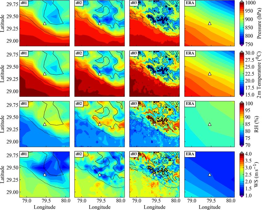
J. Singh et al.: Effects of spatial resolution on WRF v3.8.1 simulated meteorology                                            1429

non et al., 2017; Mues et al., 2018; Potter et al., 2018; Zhou      et al., 1997). For resolving the boundary layer processes the
et al., 2018, 2019; Norris et al., 2020; Wang et al., 2020), the    first-order Yonsei University (YSU) scheme based on non-
model performance over complex terrains like the Himalaya           local closure (Hong et al., 2006) is used, including an ex-
still requires improvement, which can be achieved through           plicit entrainment layer with the K-profile in an unstable
an extensive evaluation at sub-kilometer resolution against         mixed layer. The planetary boundary layer (PBL) height is
an intensive field campaign. The main objectives of the study       determined from the Richardson number (Rib ) method in
are as follows:                                                     this PBL scheme. Convection is parameterized by the Kain–
                                                                    Fritsch (KF) cumulus parameterization (CP) scheme, ac-
    1. to examine the model performance over the CH at vary-        counting for sub-grid-level processes in the model such as
       ing resolutions (15, 5 and 1 km) by evaluating several       precipitation, latent heat release, and the vertical redistribu-
       model diagnostics against the observations made during       tion of heat and moisture as a result of convection (Kain,
       the GVAX campaign;                                           2004). With the increase in model grid resolution to less
    2. to investigate the effect of feedback from the nest to the   than 10 km (known as “grey area”), the CP scheme is usu-
       parent domain, as this might allow configuring a model       ally turned off, and cloud and precipitation processes are re-
       setup covering the larger Indian region with more accu-      solved by the microphysics (MP) scheme (Weisman et al.,
       rate results over the Himalaya; and                          1997). In the present study, the CP scheme is used for d01,
                                                                    while it is turned off for d02 and d03. The Thomson mi-
    3. downscaling to a sub-kilometer (333 m) resolution with       crophysics scheme containing prognostic equations for cloud
       the implementation of a very high-resolution (3 s) topo-     water, rainwater, ice, snow, and graupel mixing ratios is used
       graphical input into the model to examine the potential      (Thompson et al., 2004). Parameterization of surface pro-
       of simulations in reproducing local-scale dynamics.          cesses is done with the MM5 Monin–Obukhov scheme and
                                                                    unified Noah land surface model (LSM) (Chen and Dudhia,
   The subsequent section (Sect. 2) describes the model             2001; Ek et al., 2003; Tewari et al., 2004). The Noah LSM
setup, followed by the experimental design and a discus-            includes a single canopy layer and four soil layers at 0.1, 0.2,
sion of datasets used for model evaluation. Section 3 pro-          0.6, and 1 m within 2 m of depth (Ek et al., 2003).
vides a comparison of model results with the ERA-Interim               The model is configured with three domains of 15 km
reanalysis (Sect. 3.1), radiosonde observations (Sect. 3.2),        (d01), 5 km (d02), and 1 km (d03) horizontal grid spacing us-
and ground-based measurements (Sect. 3.3). Analysis of              ing Mercator projection centering at Manora Peak (79.46◦ N,
domain feedback is presented in Sect. 3.4, and the effect           29.36◦ E; ∼ 1936 m a.m.s.l.) in the central Himalaya. The to-
of implementing high-resolution topography is investigated          pography within the model domains is highly complex, as
in Sect. 3.5, followed by the summary and conclusions in            evident from the ridges (Fig. 1). The outer domain d01 in-
Sect. 4.                                                            cludes the northern part of the Thar Desert, part of Indo-
                                                                    Gangetic Plain (IGP), and the Himalayan mountains, while
2     Methodology                                                   the innermost domain d03 consists of mostly mountainous
                                                                    terrain. The model has 51 atmospheric vertical levels with
2.1    Model setup and experimental design                          the top at 10 hPa. For d01, 100 east–west and 86 north–south
                                                                    grid points are used to account for the effect of synoptic-
The WRF model version 3.8.1 has been used in the present            scale meteorology, e.g., the Indian summer monsoon. The
study. WRF is a mesoscale, non-hydrostatic, numerical               d02 has 88 east–west and 76 north–south grid points cover-
weather prediction (NWP) model with advanced physics and            ing a sufficient spatial region around the observational site to
numerical schemes for simulating meteorology and dynam-             consider the effects of mesoscale dynamics, e.g., changes in
ics. WRF-ARW uses an Eulerian mass-based dynamical core             wind pattern due to orography. The innermost domain, d03,
with terrain-following vertical coordinates (Skamarock et al.,      has 126 east–west and 106 north–south grid points to resolve
2008). ERA-Interim reanalysis from the European Centre for          local effects, e.g., convection, advection, turbulence, and or-
Medium-Range Weather Forecasts (ECMWF), available at                thographic lifting.
a temporal resolution of 6 h and a horizontal resolution of            For d01, boundary conditions are provided from the ERA-
0.75◦ × 0.75◦ with 37 vertical levels from the surface to the       Interim reanalysis, as explained earlier. Model simulations
top at 1 hPa (Dee et al., 2011), has been used to provide the       have been performed for the 4 months of the summer mon-
initial and lateral boundary conditions to the WRF model.           soon: 1 June 2011 to 30 September 2011 (JJAS). This sim-
Static geographical data from the Moderate Resolution Imag-         ulation period is chosen considering the availability of con-
ing Spectroradiometer (MODIS), available at 30 s horizontal         tinuous observations from 11 June 2011 and to allow a suffi-
resolution, are utilized for land use and land cover.               cient spin-up time of 10 d for the model to achieve its equi-
   The Goddard scheme is used for shortwave radiation               librium state (Angevine et al., 2014; Seck et al., 2015; Jerez
(Chou and Suarez, 1994), while longwave radiation is sim-           et al., 2020). Only the outer domain d01 is nudged with the
ulated by the rapid radiative transfer model scheme (Mlawer         global reanalysis for temperature, water vapor, and the zonal

https://doi.org/10.5194/gmd-14-1427-2021                                              Geosci. Model Dev., 14, 1427–1443, 2021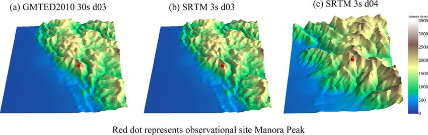
1430                                       J. Singh et al.: Effects of spatial resolution on WRF v3.8.1 simulated meteorology

Figure 1. Topography represented in the WRF model domains (a) with three horizontal resolutions, namely domain d01 (15 × 15 km),
domain d02 (5 × 5 km), and domain d03 (1 × 1 km). Each box inside a panel corresponds to the nested domain. The triangle in the innermost
box indicates the location of the GVAX campaign site, i.e., Manora Peak in Nainital. The bottom panels (b, c, d) indicate the topography of
each individual domain (left to right). The finest nest inside d03 (d) is d04 at the resolution of 333 m (discussed in Sect. 3.5).

and meridional (u and v) components of the wind using a                 (Naja et al., 2016). The continuous vertical profiles of the
nudging coefficient of 0.0006 (6 × 10⁻⁴ ) at all vertical levels        meteorological parameters except wind speed and direction
(e.g., Kumar et al., 2012). Several of the configuration op-            were available from the end of June 2011 through the en-
tions, e.g., physics and meteorological nudging, are selected           tire study period, whereas valid and quality wind data were
following earlier applications of this model over this region           available only for September 2011. Hence, in this study, ra-
(e.g., Kumar et al., 2012; Ojha et al., 2016; Singh et al., 2016;       diosonde measurements from 1 July 2011 onwards are used
Sharma et al., 2017).                                                   for the model evaluation of meteorological parameters, ex-
                                                                        cept wind speed and direction, which are evaluated only for
2.2    Observational data                                               September. A total of 309 valid profiles of temperature and
                                                                        relative humidity and 104 profiles of wind are used. Statis-
We utilize observations during an intensive field campaign –            tical metrics such as the mean bias (MB), root mean square
the Ganges Valleys Aerosol Experiment (GVAX) – to eval-                 error (RMSE), and correlation coefficient (r) are used for the
uate model simulations. The GVAX campaign was carried                   model evaluation, and a description of these metrics is given
out using the Atmospheric Radiation Measurement (ARM)                   in the Supplement.
Climate Research Facility of the U.S. Department of En-
ergy (DOE) from 10 June 2011 to 31 March 2012 at ARIES,
Manora Peak in Nainital (e.g., Kotamarthi, 2013; Singh et al.,          3     Results and discussion
2016; Dumka et al., 2017). This observational site (79.46◦ N,
29.36◦ E; 1940 m above sea level) is located in the central             3.1    Comparison with ERA-Interim reanalysis
Himalaya, as shown in Fig. 1. The surface-based meteoro-
logical measurements of ambient air temperature, pressure,              Here, we have used the ERA-Interim data for comparison
relative humidity, precipitation, and wind (speed and direc-            with WRF output. We first compare the WRF-simulated spa-
tion) were made using an automatic weather station at 1 min             tial distribution of meteorological parameters (surface pres-
temporal resolution. The instantaneous values of the observa-           sure, 2 m air temperature, 2 m RH, and 10 m WS) with the
tions are compared with hourly instantaneous model output               ERA-Interim reanalysis over the common region of all the
at the nearest grid point.                                              domains averaged for the entire simulation period (Fig. 2).
   The vertical profiles of temperature, pressure, rela-                The three contours of the topographic height of 500, 1500,
tive humidity, and horizontal wind (speed and direction)                and 2000 m are used to relate the meteorological features
were obtained by four launches (00:00, 06:00, 12:00, and                to the resolved topography in three domains. The common
18:00 UTC) of the radiosonde each day during the campaign               area in all domains includes the low-altitude IGP region in

Geosci. Model Dev., 14, 1427–1443, 2021                                                  https://doi.org/10.5194/gmd-14-1427-2021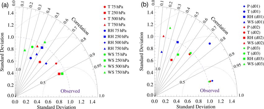
J. Singh et al.: Effects of spatial resolution on WRF v3.8.1 simulated meteorology                                          1431

the south (elevation of less than 400 m; Fig. 1) and elevated      d01 (77 %–93 %), d02 (74 %–95 %), and d03 (70 %–96 %)
mountains of the central Himalaya in the north. Also, for a        are generally comparable. The mountain slopes provide up-
consistent comparison, model-simulated values are taken at         lift to the moist monsoonal air that on ascent subsequently
the same time intervals as in ERA-Interim data (i.e., every        saturates and increases the relative humidity to about 90 %
6 h). From the comparison presented in Fig. 2, it is evident       as observed over the grid encompassing the site. Contour
that the meteorological parameters simulated by the model          lines (1500 and 2000 m in Fig. 2) depict the low pressure
are dependent on the model grid resolution. The existence          and temperature with the higher relative humidity feature of
of the sharp-gradient topographic height (SGTH) of about           the peaks, and these features are sharper as the resolution in-
1600 m from the foothill of the Himalaya to the observa-           creases from d01 to d03.
tional site modifies the wind pattern and moisture content            The wind speed is highly dependent upon the model grid
differently at different grid resolutions, indicating the crit-    resolution and orography-induced circulations during differ-
ical role of mountain orography. The surface pressure ex-          ent seasons (Solanki et al., 2016, 2019), and this is reflected
plicitly depends upon the elevation of a location from mean        in Fig. 2. As mentioned earlier, although the topography of
sea level. The contour of the pressure parameter from ERA-         the IGP region does not vary abruptly, the magnitude of the
Interim data shows the surface pressure of about 900 hPa for       wind speed over this region and over the complex Himalayan
the observational site Manora Peak, and it varied from 550 to      region is found to change significantly at different model res-
975 hPa within this region, while WRF-simulated pressure is        olutions, thereby indicating that the wind speed is very sen-
869, 835, and 827 hPa for d01, d02, and d03, respectively.         sitive to both model resolution and topography. The wind
WRF-simulated surface pressure ranges from 821.9 hPa over          speed in d01 varies from 1.3 to 2.8 m s−1 , while the wind
the high-altitude CH region to 977.0 hPa in the IGP region         variations in domains d02 (1.2–3.4 m s−1 ) and d03 (1.3–
within d01. Simultaneously, the range of variation in the sur-     4.2 m s−1 ) show higher variability than that in ERA-Interim
face pressure is 788.1–977.5 and 760.4–977.7 hPa within d02        (1.2–2.3 m s−1 ) due to finer resolution of the WRF. Overall,
and d03, respectively, and the minimum pressure decreases          the impact of the topography resolved at higher resolution in
from d01 to d03, which is attributed to the improvement            WRF shows the contrasting differences in surface pressure,
in resolved topography on increasing model grid resolution.        temperature, relative humidity, and wind speed compared to
However, the effects of the SGTH are not observed for tem-         the coarse-resolution ERA-Interim dataset.
perature, wind, and RH in ERA-Interim contours due to the
unresolved topographic features. Simulated maps show the           3.2   Comparison with radiosonde observations
spatial homogeneity of meteorological parameters over the
flat terrain of IGP in the foothills of the Himalaya compared      The intensive radiosonde observations made during the
to the elevated central Himalayan region.                          GVAX field campaign at Manora Peak (79.46◦ N, 29.36◦ E;
   The effect of spatial resolution is clearly observed over the   ∼ 1936 m a.m.s.l.) in the central Himalaya (shown in Fig. 1)
mountainous region of the Himalaya, where the size of the          are used for the evaluation of model resolutions. The com-
mountains changes abruptly, with the modeled output show-          parison of the model-simulated profiles of temperature, rela-
ing increasingly distinct features with increasing grid reso-      tive humidity, and wind speed against the radiosonde obser-
lution. On the other hand, there are minimal differences in        vations is shown in Fig. 3.
the topography of the IGP, and hence the meteorological fea-          The inversion of temperature at the top of the troposphere
tures associated with the topography are well captured in the      occurred at ∼ 90 hPa (∼ 16 km) in observations (Figs. 3d,
model even at a coarser resolution of 15 km.                       S1), whereas radiosonde profiles show that temperature de-
   Model simulations show the topography-dependent spatial         creases with pressure from 15.5 ◦ C at 750 hPa to −78.0 ◦ C
variation in 2 m temperature in the ranges of 20.0–29.5 ◦ C        at ∼ 90 hPa. As evident from the simulated temperature pro-
in d01,17.3–29.6 ◦ C in d02, and 15.5.0–29.9 ◦ C in d03, with      files, the WRF model captured these features well and was
the lowest values simulated over the elevated mountain peaks       found to show a reduction from 15.1 to −76.6 ◦ C in these
and higher values over the temperate IGP region. The con-          pressure levels. Further, the differences between model (d01)
tours in three model domains show an explicit dependency           and radiosonde observations (Fig. 3g) range from −4 to
of 2 m temperature on the grid resolution over the mountain-       4 ◦ C. The mean RH values from the radiosonde observations
ous region. With increasing model resolution, the topogra-         (model d01) also show a decrease from 82.3 % (76.7 %) at
phy is resolved to a greater extent, and lower temperature         750 % to 25.2 % (32.0 %) at 90 hPa. The mean RH difference
is simulated at higher surface elevations, as expected. Fur-       between observations and the model (Fig. 3h) shows that the
ther, the estimation of water vapor is essentially needed for      model simulates a more humid atmosphere at higher alti-
both climate and numerical weather prediction (NWP) appli-         tudes while showing a low humidity bias at lower altitudes.
cations. Figure 2 shows that the simulated relative humidity       The wind data from radiosonde measurements available for
is above 70 % in all three domains for the monsoon season.         September 2011 were utilized to compare the model out-
The variations (minimum–maximum) in the relative humid-            put. Observations and modeled winds are ≤ 10 m s−1 within
ity in the ERA-Interim (80 %–85 %) dataset over the domains        the altitude region of the surface to about 400 hPa (∼ 7 km)

https://doi.org/10.5194/gmd-14-1427-2021                                             Geosci. Model Dev., 14, 1427–1443, 2021
1432                                       J. Singh et al.: Effects of spatial resolution on WRF v3.8.1 simulated meteorology

Figure 2. Contours in the first three columns show WRF results for the three domains (first column: d01, second column: d02, third column:
d03), and the fourth column shows corresponding parameters from the ERA-Interim reanalysis. The first row shows mean surface pressure
during the monsoon (JJAS), the second row shows 2 m temperature (in ◦ C), the third row shows 2 m relative humidity (RH; %), and the
bottom row shows 10 m wind speed (WS; m s−1 ) along with three elevation contours at 500 m (dashed), 1500 m (thin solid), and 2000 m
(thick solid).

until the middle of September (day of the year 258). Wind              (r = 0.71) but shows poor correlation at 75 hPa (r = 0.17)
increases (≥ 15 m s−1 ) above 400 hPa and attains maximum              near the model top.
values (≥ 25 m s−1 ) between 250 and 100 hPa after 258 d of               Lower correlations for temperature and wind speed near
the year (15 September 2011). However, simulated winds are             the surface (750 hPa) could be due to terrain-induced effects,
slightly lower and less widespread compared to observations.           which are most significant in the local boundary layer. The
The comparison of the wind profiles with the same x axis               surface-level winds and turbulence are some of the bound-
(shown in Fig. S2) as other meteorological parameters shows            ary layer features affected mainly by the surface and terrain
that lower relative humidity (0.80) than that at lower alti-             Figure 5 shows the vertical profiles of the following statis-
tudes, i.e., 750 hPa (r
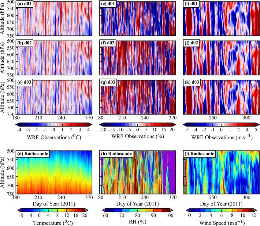
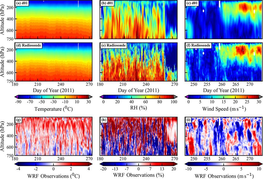
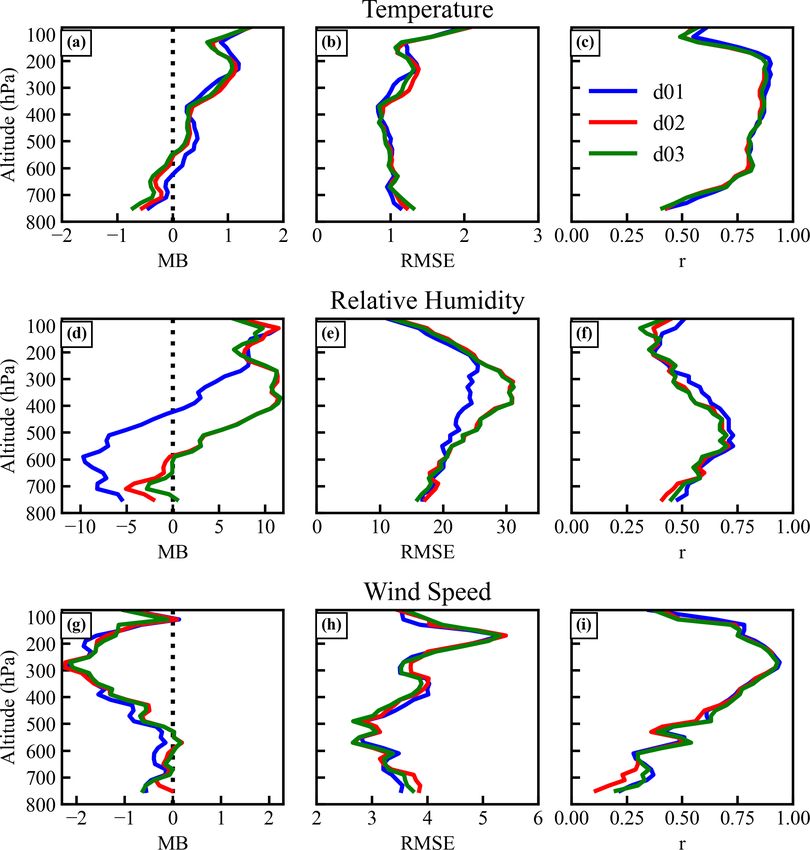
J. Singh et al.: Effects of spatial resolution on WRF v3.8.1 simulated meteorology                                                    1433

Figure 3. The comparison of simulated vertical profiles of (a) temperature (◦ C), (b) relative humidity (RH; %), and (c) wind speed (m s−1 )
in d01 with the radiosonde observations (d, e, f). The x axis in (a), (b), (d), (e), (g), and (h) shows the day of the year in 2011 starting
from 1 July (182nd day) to 30 September (273rd day). The vertical profiles of wind speed (c, f) are plotted only for September 2011. The
third row (g, h, i) shows the difference in temperature, relative humidity, and wind speed between the WRF d01 simulation and radiosonde
observations.

speed. The magnitudes of the MB values throughout the tro-              The effect of model resolution is not very significant for tem-
posphere are estimated to be within about 1 ◦ C, 12 %, and              perature and wind profiles above 800 hPa; nevertheless, the
2.5 m s−1 for temperature, relative humidity, and wind speed,           mean bias for RH is lower (∼ 5 %) in the 800–600 hPa al-
respectively. Additionally, RMSE values are about 1 ◦ C,                titude range and higher in the 450–300 hPa altitude range
15 %–30 %, and 2.5–5 m s−1 for temperature, relative humid-             in the d02 and d03 simulations. This might be due to deep
ity, and wind speed, respectively. As discussed earlier, corre-         convection in the model at a higher resolution. Overall, the
lations between model results and observations are found to             model captured the vertical structures of meteorological pa-
be stronger in the middle and upper troposphere than in the             rameters; however, a better representation of complex ter-
lower troposphere. For temperature, the r values are higher             rain is insufficient to improve the model performance aloft.
than 0.75 between 600 and 200 hPa, whereas they decrease                On top of the better representation of topography as con-
to 0.4 at lower altitudes, i.e., near 800 hPa. Correlations in          sidered here, it highlights the need for future studies eval-
the lower troposphere are notably weaker (r = ∼ 0.25) in the            uating various physics scheme. Nevertheless, model biases
case of wind speed. The results suggest that the model cap-             have been significantly reduced for surface-level meteorol-
tures the day-to-day variabilities well in the meteorological           ogy with higher resolution, and the details are discussed in
parameters in the middle and upper troposphere and to a mi-             the subsequent section.
nor extent in the lower troposphere. Relatively weaker cor-
relations in the lower troposphere are suggested to be as-              3.3    Comparison with ground-based observations
sociated with more pronounced effects of the uncertainties
caused by the underlying complex mountain terrain and re-               The model-simulated 2 m temperature (T 2), 2 m relative hu-
sulting unresolved local effects. Wind fields near the surface          midity (RH2), and 10 m wind speed (WS10) for the obser-
are strongly impacted by interactions between the terrain and           vational site, Manora Peak, are compared with the ground-
boundary layer in addition to orographic drag in a model-               based measurements made during the GVAX campaign in
ing study over the Tibetan Plateau (Zhou et al., 2018) and              Fig. 6 and summarized in Table 1. The diurnal variations in
in measurements over the Himalaya (Solanki et al., 2019).               T 2, RH2, and WS10 simulated by the WRF model are com-
An increase in bias with altitude was reported by Kumar                 pared with observations, whereas the surface pressure does
et al. (2012) for dew point temperature. Besides the model              not show a significant diurnal variation (not shown here).
physics, the higher uncertainties in radiosonde humidity ob-            Model simulation d01 shows a positive bias of 68 hPa in sur-
servations might have also contributed to these differences.            face pressure, with a strong correlation (r = 0.97) with ob-

https://doi.org/10.5194/gmd-14-1427-2021                                                    Geosci. Model Dev., 14, 1427–1443, 2021
1434                                        J. Singh et al.: Effects of spatial resolution on WRF v3.8.1 simulated meteorology

Figure 4. Difference between model (d01: first row, d02: second row, d03: third row) and radiosonde observations for temperature (a, b,
c), relative humidity (e, f, g), and wind speed (i, j, k) profiles up to 500 hPa. The fourth row provides the vertical profiles of radiosonde
measurements. The x axis in panels (a–h) shows the day of the year in 2011 from 1 July (182nd day) to 30 September (273rd day). Wind
speed (m s−1 ) profiles in panels (i–l) are provided for September 2011.

servations (mean = ∼ 801 hPa). A significant improvement                 and spatial scales. The average 10 m wind speed (WS10)
is achieved (MB = 26 hPa) in d03 as a result of the finest-              during the monsoon over the measurement station is about
resolution simulation (Fig. 6 and Table 1). The WRF-model-               2.1 ± 1.4 m s−1 , which is quite comparable to that simulated
simulated T 2 shows a warm bias in all three domains. The                in d01 (2.1 ± 1.1 m s−1 ), whereas it is overestimated in d02
simulated T 2 for d01 varies from 16.2 to 28.7 ◦ C, with a               by 0.9 m s−1 and in d03 by 0.5 m s−1 (Tables 1 and S1). In
higher mean value of 22.3 ± 2.1 ◦ C compared to the observed             the case of the WS10, the correlation is 0.18 for d01 and
mean value of 19.5 ± 1.6 ◦ C and a correlation of r = 0.75 be-           d02, which improves to 0.24 in d03. The diurnal variation of
tween d01 and observations. This warm bias is seen to de-                WS10 (Fig. 6c) is not well captured, especially during noon-
crease from d01 (2.8 ◦ C) to 0.2 ◦ C with increasing model res-          time.
olution in the d03 simulation (Table S1). The mean value                    Due to the complex terrain and the grid size of the model,
of the RH2 in d01 is about 88.2 ± 9.7 %, which is 6.4 %                  the simulated altitude of the observational site could differ
lower than the observed value of 94.7 ± 9.5 % with a cor-                from reality. In this study, the model underestimated sta-
relation of about 0.45 (Fig. 7b). MB and RMSE values of                  tion altitude by about 588, 480, and 270 m in d01, d02, and
RH2 show a decrease with increasing model resolution (Ta-                d03. We performed an additional evaluation to explore and
ble S1). As relative humidity also depends on temperature,               achieve possible improvement by linearly interpolating the
the diurnal variation in 2 m specific humidity (Q2; g kg−1 )             vertical profile of meteorological parameters to the actual al-
has also been analyzed (Fig. S3). Q2 is observed in the range            titude of the station (Fig. 6d–f), as done in a few previous
of 5.5–21.5 g kg−1 with a mean value of 16.8 ± 2.0 g kg−1 .              studies (e.g., Mues et al., 2018). The altitude adjustment was
It is found that the agreement in Q2 is relatively better                made as per the equation of linear interpolation given in the
(MB = −0.7 g kg−1 ; r = 0.77 in d03) when the statistical                Supplement (Eq. 4). The analysis shows that the correlation
metrics are compared with those for RH2 (Table S1). The                  coefficient values between the model and observations do not
wind speed plays a vital role in transport processes and con-            show any clear improvement in model output (e.g., for T 2
trols the dynamics of the atmosphere at different temporal               the correlation coefficient is 0.35) on adjusting the altitude

Geosci. Model Dev., 14, 1427–1443, 2021                                                    https://doi.org/10.5194/gmd-14-1427-2021
J. Singh et al.: Effects of spatial resolution on WRF v3.8.1 simulated meteorology                                                    1435

Table 1. The mean (±standard deviation) along with the minimum and maximum values of the meteorological parameters surface pressure
(P ; hPa), 2 m temperature (T 2; ◦ C); 2 m relative humidity (RH2; %), and 10 m wind speed (WS10; m s−1 ) in the model simulations and
observations for the full observation period. An additional evaluation is presented, accounting for the difference in model surface altitude
and the actual altitude of measurements (referred to as “with altitude adjustment”).

        Parameter                 Without altitude adjustment                    With altitude adjustment              Observation
                                  d01             d02            d03             d01             d02            d03
        P (hPa)           869.6 ± 2.6     835.3 ± 2.5    827.6 ± 2.4    801.3 ± 2.4.6    801.3 ± 2.4    801.4 ± 2.4    801.1 ± 2.4
        Min/max           862.8/875.1     828.3/840.8    821.2/833.1     795.0/806.7     795.0/806.7    795.2/806.8    795.1/806.8
        T 2 (◦ C)          22.3 ± 1.8      20.4 ± 1.8     19.8 ± 1.1       18.4 ± 0.8     18.4 ± 0.9     18.3 ± 0.9     19.5 ± 1.1
        Min/max             16.2/28.7       15.1/26.0      14.0/25.0        16.1/20.9      15.5/21.8      15.6/22.1      14.8/25.6
        RH2 (%)            88.2 ± 9.7      94.3 ± 6.4     92.3 ± 7.9     86.2 ± 10.9      93.8 ± 8.5     91.5 ± 9.7     94.7 ± 9.5
        Min/max              53.3/100        67.6/100       52.3/100         43.9/100       51.3/100       47.9/100       31.6/100
        WS10 (m s−1 )       2.1 ± 1.1       3.0 ± 1.4      2.6 ± 1.7        3.4 ± 2.6      4.8 ± 3.1      4.0 ± 3.1      2.1 ± 1.4
        Min/max               0.0/8.6        0.1/11.4        0.1/11.7        0.0/20.2       0.1/23.9       0.1/22.1       0.0/10.0

                                                                        not achieved (Table S1); instead, the absolute values of biases
                                                                        increase from 0.2 to 1.2, 2.4 to 3.1, 0.5 to 1.9, and 0.7 to 1.6
                                                                        in T 2, RH2, WS10, and Q2 in simulation d03. Besides ther-
                                                                        mal and mechanical interactions of mountain surfaces with
                                                                        the atmosphere, local processes such as evaporation and tran-
                                                                        spiration affect the near-surface meteorological conditions. A
                                                                        reduction in wind speed during the daytime is associated with
                                                                        the competing effects of mountain–valley circulations due to
                                                                        heating of the slopes versus synoptic-scale flows (Solanki
                                                                        et al., 2019). To resolve such sub-grid-scale processes, we
                                                                        emphasize that very high-resolution simulations are needed,
                                                                        as conducted in this study, in order to simulate the meteoro-
                                                                        logical variability in a satisfactory way. The analysis further
                                                                        highlights the need for accurate representation of the com-
                                                                        plex topographical features rather than altitude-adjusted esti-
                                                                        mations, which led to very limited improvements in this case.
                                                                        However, we will discuss the evaluation without altitude ad-
                                                                        justment unless stated otherwise.
                                                                           We evaluate the MB values (Tables 1 and S1) in model
                                                                        simulations considering the benchmarks suggested by Emery
                                                                        et al. (2001). In the d03 simulation, MB values for both
                                                                        T 2 (0.2 ◦ C) and Q2 (−0.7 g kg−1 ) are found to be well
Figure 5. The vertical profiles of the mean bias (MB), root mean        within the range of benchmark values: ±0.5 ◦ C for T 2 and
square error (RMSE), and correlation coefficient (r) for tempera-
                                                                        ±1.0 g kg−1 for Q2. It is important to note that biases in T 2
ture, relative humidity, and wind speed in the different domains d01
(blue), d02 (red), and d03 (green).
                                                                        in the coarser simulations d01 (2.8 ◦ C) and d02 (0.9 ◦ C) are,
                                                                        however, higher compared to the benchmarks. MB values in
                                                                        T 2 estimated for this representative Himalayan site are found
                                                                        to be slightly lower (+0.2 ◦ C) (−1.2 ◦ C with altitude adjust-
except for WS10. After adjusting the altitude, the tempera-             ment) than those over the Tibetan Plateau (−2 to −5 ◦ C)
ture variability is suppressed by the model at diurnal (Fig. 6a,        (Gao et al., 2015) and over mountainous regions in the Eu-
d) and day-to-day timescales; i.e., r drops from 0.67 to 0.36           rope (Zhang et al., 2013). The warmer bias in our case is due
in d03. The comparison of temperature among the three do-               to underestimation of the Himalayan altitude, whereas the
mains for additional model layers has also been analyzed                model overestimated terrain height over the Tibetan Plateau
(Fig. S4). The diurnal amplitudes are seen to be smaller at             region, giving contrasting results. Further, the RMSE in wind
higher model layers. Additionally, the differences among dif-           speed is lower (1.6–2.0 m s−1 ) than that over the Kathmandu
ferent simulations (d01, d02, and d03) also decrease at higher          valley (2.2 m s−1 ; Mues et al., 2018) and similar to the bench-
layers. As expected, the altitude adjustment does reduce the            mark (2.0 m s−1 ). Mar et al. (2016) also reported a similar
bias in pressure. Nevertheless, reductions in mean biases are

https://doi.org/10.5194/gmd-14-1427-2021                                                    Geosci. Model Dev., 14, 1427–1443, 2021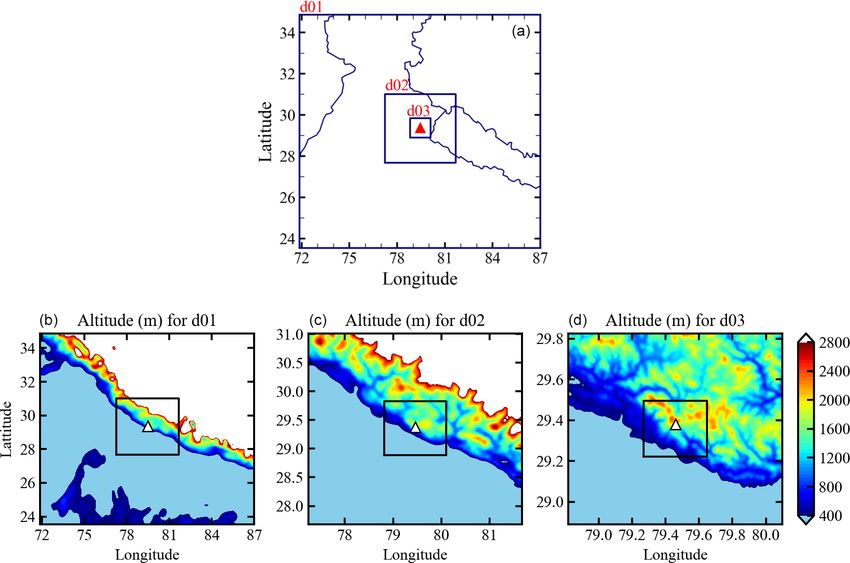
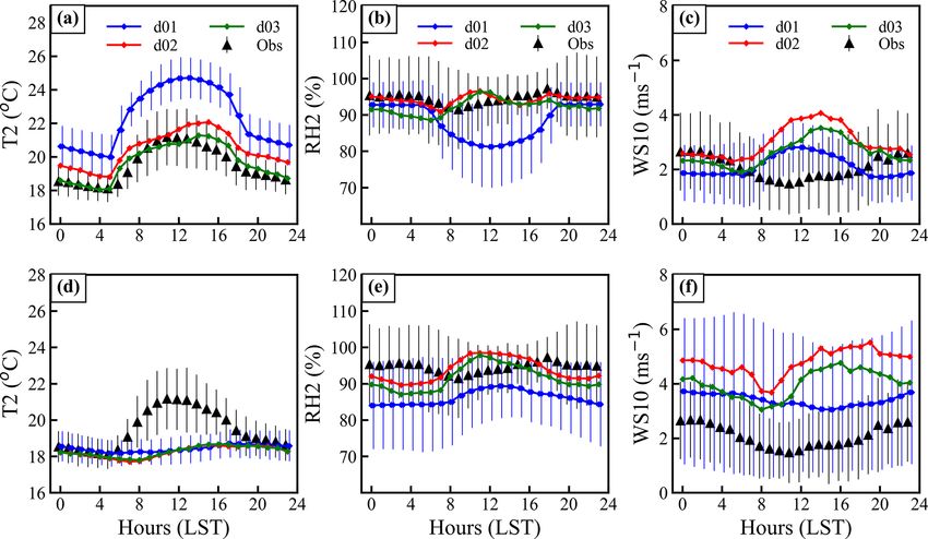
1436                                       J. Singh et al.: Effects of spatial resolution on WRF v3.8.1 simulated meteorology

Figure 6. Mean diurnal variations of (a) 2 m temperature (T 2), (b) 2 m relative humidity (RH2), and (c) 10 m wind speed (WS10) from
model simulations (d01, d02, and d03) and observations. Altitude-adjusted variations are also shown (d–f). The bars represent the standard
deviation and are shown only for domain d01 and the observations in order to avoid overlap.

bias (2 m s−1 ) in the 10 m wind speed over Europe and an              vations show that winds blowing from the north, northeast,
average correlation of ∼ 0.4–0.6 over the Alps. Nevertheless,          south, and southwest are very weak (
J. Singh et al.: Effects of spatial resolution on WRF v3.8.1 simulated meteorology 1437
Figure 7. Taylor diagram with the correlation coefficient, normalized standard deviation, and normalized root mean square difference
(RMSD) error for (a) model performance at the different pressure levels shown in Fig. 3 for d01. (b) The model-simulated surface pres-
sure, 2 m temperature, RH, and 10 m wind speed for different domains as shown in Fig. 6a–c.
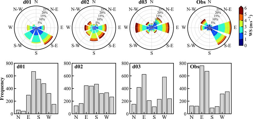
Figure 8. Comparison of the wind speed and direction represented by the wind rose (top panel) and the frequency distribution of the wind
direction (bottom panel) for model simulations over the three domains (d01, d02, d03) and observations (obs) during June–September 2011.
Different colors and radii of wind roses show the wind speed and frequency of occurrences, respectively.
lated meteorological parameters (T 2, RH2, and WS10) for Table 2. Comparison of the simulated meteorology for surface pres-
the outermost domain with surface observations is presented sure (P ), 2 m temperature (T 2), 2 m relative humidity (RH2), 10 m
in Fig. 9 for both WRF-WF and WRF-F simulations, thus wind speed (WS10), and 2 m specific humidity (Q2) to the obser-
showing the effect of feedback within the outermost domain. vations in the outermost domain d01 for two model simulations:
The comparison of mean values (Table 2) shows a de- WRF-WF and WRF-F.
crease in model bias for T 2, RH2, and Q2 by 0.5 ◦ C, 0.3 %,
Parameters Observed WRF-WF WRF-F
and 0.2 g kg−1 , respectively, due to feedback from finer-
resolution simulations. Additionally, correlations are found P (hPa) 801.4 ± 2.4 869.6 ± 2.6 858.9 ± 2.5
to show improvements for RH2 and Q2 by 0.15 and 0.12, T 2 (◦ C) 19.5 ± 1.6 22.3 ± 2.1 21.9 ± 1.4
respectively, due to feedback; hence, the diurnal variation of RH2 (%) 94.7 ± 9.5 88.2 ± 4.9 88.6 ± 4.9
relative humidity is closer to the observations (Fig. 9). Never- WS10 (m s−1 ) 2.1 ± 1.4 2.1 ± 1.1 1.7 ± 1.3
theless, smaller changes were seen in correlations for WS10 Q2 (g kg−1 ) 16.8 ± 2.0 17.3 ± 2.0 17.0 ± 2.1
(by 0.05) and T 2 (by −0.02) (Fig. S5). Variations in wind
speed and direction also show significant improvements, es-
pecially in the dominant flow direction, e.g., east, west, and over the mountainous region than over the flat terrain of the
northwest (Fig. S6). IGP. The feedback from the nested domain to the parent do-
Effects of the feedback on surface pressure, 2 m tempera- main mostly modifies the meteorology over the mountainous
ture, and relative humidity in the domain d01 are shown by region, as shown by the topography contours in Fig. 10. The
Fig. 10. Feedback effects are seen to be more pronounced analyses of biases and correlations suggest an improvement
https://doi.org/10.5194/gmd-14-1427-2021 Geosci. Model Dev., 14, 1427–1443, 20211438 J. Singh et al.: Effects of spatial resolution on WRF v3.8.1 simulated meteorology
Figure 9. Diurnal variation of the T 2, RH2, and WS10 from d01 without feedback (WRF-WF) and with feedback (WRF-F). The bars
represent the standard deviation and are shown only for domain d01 and observations in order to avoid overlap.
Figure 10. The effect of the two-way nesting on d01 is shown. The difference between the simulations with feedback (WRF-F) and without
feedback (WRF-WF) is shown for surface pressure, 2 m temperature, and 2 m relative humidity along with three elevation contours at 500 m
(dashed), 1500 m (thin solid), and 2000 m (thick solid).
in the model-simulated pressure, temperature, and humidity similar resolution using GMTED2010 (GMTED hereafter).
through feedback from well-resolved nests. This further un- For this experiment, model simulation is performed only for
derpins the fact that better representations of the Himalaya September 2011. This simulation is carried out without feed-
over local scales can be adopted to simulate meteorology at back and compared with the observation to check the effect
the regional scale with lower biases over complex terrain of implementing high-resolution topography.
in the given domain. Nevertheless, further modeling stud- The comparison of the topographic height between
ies along with more observations are needed to improve the GMTED and SRTM3s in Fig. S7 shows that the differ-
model performance. We extended the efforts to improve the ences are larger over the mountainous region, which vary
wind speed and direction simulated over the complex topog- from −100 to +100 m. The differences are suppressed within
raphy by implementing a high-resolution (3 s) topographical d02 and d03 as the topography input is changed from
input in the model to evaluate finer-resolution features over the GMTED to SRTM3s datasets. The topography in d04
the Himalaya in the following section. (Fig. 11c) becomes resolved better and is marked by sharp
variations of mountain ridges and valleys using the SRTM3s
3.5 Inclusion of high-resolution (3 s) SRTM topography compared to d03, which are smoothed out with GMTED
(Fig. 11a) or with SRTM3s interpolated to 1 km (Fig. 11b).
After including the SRTM3s topography, the MB value for
Simulations described in previous sections were per-
wind speed in d03 is found to show a slight reduction
formed using the 30 s (∼ 1 km) topographic data from the
(∼ 0.04 m s−1 ). Also, the flow from various directions exhib-
GMTED2010 (Danielson and Gesch, 2011), which is compa-
ited an improvement of 1 %–2 % with the use of SRTM3s
rable to the highest resolution of the WRF simulation (d03).
(Table S2).
In order to evaluate the influences of topographical features
In d04, surface pressure is seen to be simulated more real-
on the wind flow at finer scales, the topography input avail-
istically (809 hPa), and the dry bias in 2 m relative humidity
able at very high resolution (3 s or ∼ 90 m) from the Shuttle
is improved by ∼ 2 % (Fig. S8 and Table S2). Simulations of
Radar Topography Mission (SRTM3s) (Farr et al., 2007) has
diurnal wind variations remain challenging (not shown here)
been utilized. However, retaining the same model configu-
even at the finest resolutions considered (d04) utilizing the
ration as earlier, an additional innermost nest d04 having a
updated topographic data (SRTM3s). Further, to understand
resolution of ∼ 333 m, as depicted in Fig. 1 (bottom right
the effect of SRTM3s data on d04, the wind direction is com-
panel), is included. Simulations with SRTM data at 1 km res-
pared with that in d03 and observations. The variations in
olution did not differ significantly from the simulation with a
Geosci. Model Dev., 14, 1427–1443, 2021 https://doi.org/10.5194/gmd-14-1427-2021J. Singh et al.: Effects of spatial resolution on WRF v3.8.1 simulated meteorology 1439
Figure 11. The topography from GMTED at 30 s in domain d03 (a), SRTM at 3 s in domain d03 (b), and SRTM at 3 s in domain d04 (c).
The model elevations of the observational site in d03 and d04 are 1670 and 1876 m, respectively.
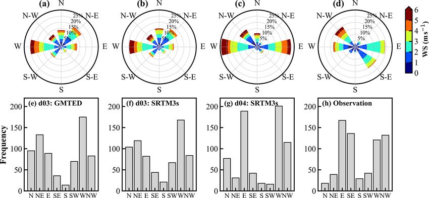
winds are analyzed and shown by a wind rose (Fig. 12a–d) comparison of model results to an intensive field campaign,
and frequency distribution (Fig. 12e–h). The fraction of the and downscaling to a sub-kilometer resolution with 3 s reso-
northeasterly component in d04 with SRTM3s (5 %) is found lution SRTM topography data that resolves individual peaks
to be comparable with observations (6 %), which was over- and valleys over the CH region. The effects of spatial res-
estimated by 19 % (17 %) in d03 with GMTED (SRTM3s). olution on model-simulated meteorology have been exam-
The frequency of the southerlies improves with the increas- ined by combining the WRF model with ground-based and
ing resolution of topography and better matches the obser- in situ observations, as well as reanalysis datasets. Owing
vations. The observations show the prevalence of northwest- to the highly complex topography of the central Himalaya,
erly (19 %), easterly (24 %), westerly (18 %), and southeast- model results show strong sensitivity towards the model reso-
erly (20 %) winds, and these are also seen to be the dominant lution and adequate representation of terrain features. Model-
directions in the simulation d04, with the exception of south- simulated meteorological profiles do not show much depen-
easterly winds. dency on the resolution, except in the lower atmosphere,
Simulation of the wind directions improved from d03 to which is directly influenced by terrain-induced effects and
d04 by using the SRTM3s topography, except certain wind surface characteristics, emphasizing the need to evaluate var-
directions such as southeasterly. An improvement is noticed ious physics schemes over this region. The biases in 2 m
in simulated surface pressure, 2 m relative humidity, and temperature, relative humidity, and surface pressure show
10 m wind speed using the SRTM3s topography. Topograph- a decrease on increasing the model resolution, indicating a
ical data at different resolutions are found to show RH dif- better-resolved representation of topographical features. Di-
ferences in the range of −1 % to 1 % in d02 and −3 % to urnal variations in meteorological parameters also show bet-
3 % in d03 (Fig. S9). Differences in simulated RH could be ter agreement on increasing the grid resolution. Although the
associated with the multi-scale orographic variations, which surface pressure does not show a pronounced diurnal vari-
are found to be the key factors in meteorological simulation ation, the biases in simulated surface pressure are signifi-
over complex terrain (e.g., Wang et al., 2020). The effects of cantly reduced over fine-resolution simulations. Interpolation
the SRTM3s topographic static data have been studied pre- of coarser simulations (d01, d02) to the station altitude re-
viously over other regions of the world (e.g., Teixeira et al., duces the bias in surface pressure and temperature, but it sup-
2014; De Meij and Vinuesa, 2014). However, the lower day- presses the diurnal variability. The results highlight the sig-
time wind speed and the transition phases during morning nificance of accurately representing terrains at finer resolu-
and evening hours still remain a challenge, even after using tions (d03). The model is generally not able to reproduce the
the high-resolution (333 m × 333 m) nest. Such discrepan- frequency distribution of the wind direction, except in some
cies between the model and observations over the Himalayan of the major components in all the simulations with varying
region are suggested to be associated with still unresolved resolutions. The directionality of the simulated winds shows
terrain features, in addition to the influences of input mete- improvements over finer grid resolutions; however, reproduc-
orological fields and the model physics on simulated atmo- ing the diurnal variability still remains a challenge. Biases
spheric flows (e.g., Xue et al., 2014; Vincent and Hahmann, are stronger typically during daytime and also during transi-
2015). tions of low to high wind conditions and vice versa. This is
attributed to the uncertainties in representing the interaction
of slope winds with the synoptic mean flow and local cir-
4 Summary and conclusions culations, despite an improved representation of terrain fea-
tures. A sensitivity experiment with domain feedback turned
This study using the WRF model mainly elucidated upon the on shows that the feedback process can improve the repre-
various diagnostics it calculates for its multiple domains, the sentation of the CH in simulations covering a larger region
https://doi.org/10.5194/gmd-14-1427-2021 Geosci. Model Dev., 14, 1427–1443, 20211440 J. Singh et al.: Effects of spatial resolution on WRF v3.8.1 simulated meteorology
Figure 12. Wind roses for (a) d03 using GMTED, (b–c) d03 and d04 using SRTM3s topography data, and (d) surface observations. The
corresponding frequency distributions of the wind directions are shown in (e–f). The comparison of the wind speed and direction is shown
for the month of September in 2011.
of the northern Indian subcontinent. It is suggested that fur- Acknowledgements. We are thankful to the director of ARIES,
ther improvements in the model performance are limited due Nainital. We acknowledge NCAR for the WRF-ARW model,
to the lack of high-resolution topographical biases through ECMWF for the ERA-Interim reanalysis datasets, and the ARM
input meteorological fields and model physics. Nevertheless, Climate Research Facility of the U.S. Department of Energy (DOE)
the implementation of a very high-resolution (3 s) topograph- for the observations made during the GVAX campaign. Comput-
ing resources from the Max Planck Computing and Data Facility
ical input using the SRTM data shows the potential to reduce
(MPCDF) are profoundly acknowledged. Narendra Ojha acknowl-
the biases related to topographical features to some extent. edges the computing resources Vikram-100 HPC at the Physical
Research Laboratory (PRL) and valuable support from Duggirala
Pallamraju and Anil Bhardwaj. Constructive comments and sug-
Code and data availability. Observational data from the GVAX gestions from the anonymous reviewers and the handling editor are
campaign are freely available (https://adc.arm.gov/discovery/#v/ gratefully acknowledged.
results/s/fsite::pgh.M, Kotamarthi, 2013). WRF is an open-source
and publicly available model, which can be downloaded at http:
//www2.mmm.ucar.edu/wrf/users/download/get_source.html (Ska-
Financial support. Jaydeep Singh is the senior research fellow for
marock et al., 2008). A zip file containing (a) namelists for both
the ABLN&C:NOBLE project under ISRO-GBP.
the preprocessor (WPS) and the WRF (b) 3 s resolution topogra-
phy input prepared for the pre-processor, along with a README
The article processing charges for this open-access
file describing the necessary details to perform the simulations, has
publication were covered by the Max Planck Society.
been archived at https://doi.org/10.5281/zenodo.3978569 (Singh
and Ojha, 2020).
Review statement. This paper was edited by Juan Antonio Añel and
reviewed by three anonymous referees.
Supplement. The supplement related to this article is available on-
line at: https://doi.org/10.5194/gmd-14-1427-2021-supplement.
Author contributions. NS and AP designed and supervised the References
study. JS performed the simulations, assisted by NO and AS. JS,
NO, and AS analyzed the model results, and NKK, KR, and SSG Angevine, W. M., Bazile, E., Legain, D., and Pino, D.: Land surface
contributed to the interpretations. VRK significantly contributed to spinup for episodic modeling, Atmos. Chem. Phys., 14, 8165–
conceiving and realizing the GVAX campaign. JS and NS wrote the 8172, https://doi.org/10.5194/acp-14-8165-2014, 2014.
first draft, and all the authors contributed to the paper. Bhutiyani, M. R., Kale, V. S., and Pawar, N. J.: Long-term trends in
maximum, minimum and mean annual air temperatures across
the Northwestern Himalaya during the twentieth century, Cli-
Competing interests. The authors declare that they have no conflict matic Change, 85, 59–177, https://doi.org/10.1007/s10584-006-
of interest. 9196-1, 2007.
Bonasoni, P., Cristofanelli, P., Marinoni, A., Vuillermoz, E.,
and Adhikary, B.: Atmospheric pollution in the Hindu Kush-
Geosci. Model Dev., 14, 1427–1443, 2021 https://doi.org/10.5194/gmd-14-1427-2021J. Singh et al.: Effects of spatial resolution on WRF v3.8.1 simulated meteorology 1441 Himalaya region: Evidence and implications for the regional cli- Ek, M. B., Mitchell, K. E., Lin, Y., Rogers, E., Grun- mate, Mt. Res. Dev., 32, 468–479, 2012. mann, P., Koren, V., Gayno, G., and Tarpley, J. D.: Im- Boyle, J. and Klein, S. A.: Impact of horizontal resolution on cli- plementation of Noah land surface model advances in the mate model forecasts of tropical precipitation and diabatic heat- National Centers for Environmental Prediction operational ing for the TWP-ICE period, J. Geophys. Res.-Atmos., 115, mesoscale Eta model, J. Geophys. Res.-Atmos., 108, D228851, D23113, https://doi.org/10.1029/2010JD014262, 2010. https://doi.org/10.1029/2002JD003296, 2003. Cannon, F., Carvalho, L. M. V., Jones, C., Norris, J., Bookha- Emery, C., Tai, E., and Yarwood, G.: Enhanced meteorologi- gen, B., and Kiladis, G. N.: Effects of topographic smooth- cal modeling and performance evaluation for two Texas ozone ing on the simulation of winter precipitation in High episodes, Technical Report, Texas Natural Resource Conserva- Mountain Asia, J. Geophys. Res.-Atmos., 122, 1456–1474, tion Commission, ENVIRON International Corporation, Work https://doi.org/10.1002/2016JD026038, 2017. Assignment No. 31984-11, ENVIRON International Corpora- Caya, D. and Laprise, R.: A semi-implicit semi-Lagrangian tion, Novato, CA, 235 pp., 2001. regional climate model: The Canadian RCM, Mon. Farr, T. G., Rosen, P. A., Caro, E., Crippen, R., Duren, R., Hensley, Weather Rev., 127, 341–362, https://doi.org/10.1175/1520- S., Kobrick, M., Paller, M., Rodriguez, E., Roth, L., and Seal, 0493(1999)1272.0.CO;2, 1999. D.: The shuttle radar topography mission, Rev. Geophys., 45, Chen, F. and Dudhia, J.: Coupling an advanced land surface – RG2004, https://doi.org/10.1029/2005RG000183, 2007. hydrology model with the Penn State – NCAR MM5 mod- Foley, A. M.: Uncertainty in regional climate mod- eling system. Part I: Model implementation and sensitivity, elling: A review, Prog. Phys. Geog., 34, 647–670, Mon. Weather Rev., 129, 569–585, https://doi.org/10.1175/1520- https://doi.org/10.1177/0309133310375654, 2010. 0493(2001)1292.0.CO;2, 2001. Gao, Y., Xu, J., and Chen, D.: Evaluation of WRF mesoscale cli- Cheng, W. Y. Y. and Steenburgh, W. J.: Evaluation of surface mate simulations over the Tibetan Plateau during 1979–2011, sensible weather forecasts by the WRF and the Eta Models J. Climate, 28, 2823–2841, https://doi.org/10.1175/JCLI-D-14- over the western United States, Weather Forecast., 20, 812–821, 00300.1, 2015. https://doi.org/10.1175/WAF885.1, 2005. Hanna, S. R. and Yang, R.: Evaluations of Mesoscale Chou, M. D. and Suarez, M. J.: An efficient thermal infrared Models’ Simulations of Near-Surface Winds, Tem- radiation parameterization for use in general circulation mod- perature Gradients, and Mixing Depths, J. Appl. Me- els, NASA Technical Memorandum No. 104606 Vol. 3, NASA, teorol., 40, 1095–1104, https://doi.org/10.1175/1520- Washington D. C., USA, 85 pp., 1994. 0450(2001)0402.0.CO;2, 2001. Christensen, J. H., Christensen, O. B., Lopez, P., van Meijgaard, Hong, S. Y., Noh, Y., and Dudhia, J.: A new vertical dif- E., and Botzet, M.: The HIRHAM4 regional atmospheric climate fusion package with an explicit treatment of entrain- model, DMI Scientific report 4, DMI, Copenhagen, Denmark, 51 ment processes, Mon. Weather Rev., 134, 2318–2341, pp., 1996. https://doi.org/10.1175/MWR3199.1, 2006. Danielson, J. J. and Gesch, D. B.: Global multi-resolution terrain Jerez, S., López-Romero, J. M., Turco, M., Lorente-Plazas, elevation data 2010 (GMTED2010) (No. 2011-1073), US Geo- R., Gómez-Navarro, J. J., Jiménez-Guerrero, P., and Mon- logical Survey, Reston, Virginia, USA, 26 pp., 2011. távez, J. P.: On the Spin-Up Period in WRF Simula- Dee, D. P., Uppala, S. M., Simmons, A. J., Berrisford, P., Poli, tions Over Europe: Trade-Offs Between Length and Sea- P., Kobayashi, S., Andrae, U., Balmaseda, M. A., Balsamo, G., sonality, J. Adv. Model. Earth Syst., 12, e2019MS001945, Bauer, D. P., and Bechtold, P.: The ERA-Interim reanalysis: Con- https://doi.org/10.1029/2019MS001945, 2020. figuration and performance of the data assimilation system, Q. J. Kain, J. S.: The Kain-Fritsch convective pa- Roy. Meteor. Soc., 137, 553–597, https://doi.org/10.1002/qj.828, rameterization: an update, J. Appl. Meteo- 2011. rol., 43, 170–181, https://doi.org/10.1175/1520- Deep, A., Pandey, C. P., Nandan, H., Purohit, K. D., Singh, N., 0450(2004)0432.0.CO;2 ,2004. Singh, J., Srivastava, A. K., and Ojha, N.: Evaluation of ambi- Kotamarthi, V. R.: Ganges Valley Aerosol Experiment (GVAX) ent air quality in Dehradun city during 2011–2014, J. Earth Syst. Final Campaign Report DOE/SC-ARM-14-011, available at: Sci., 128, 96, https://doi.org/10.1007/s12040-019-1092-y, 2019. https://adc.arm.gov/discovery/#v/results/s/fsite::pgh.M (last ac- De Meij, A. and Vinuesa, J. F.: Impact of SRTM cess: January 2021), 2013. and Corine Land Cover data on meteorological pa- Kumar, A., Singh, N., Anshumali, and Solanki, R.: Evaluation and rameters using WRF, Atmos. Res., 143, 351–370, utilization of MODIS and CALIPSO aerosol retrievals over a https://doi.org/10.1016/j.atmosres.2014.03.004, 2014. complex terrain in Himalaya, Remote Sens. Environ., 206, 139– Dimri, A. P., Chevuturi, A., Niyogi, D., Thayyen, R. J., Ray, K., 155, https://doi.org/10.1016/j.rse.2017.12.019, 2018. Tripathi, S. N., Pandey, A. K., and Mohanty, U. C.: Cloud- Kumar, R., Naja, M., Pfister, G. G., Barth, M. C., and Brasseur, bursts in Indian Himalayas: a review, Earth-Sci. Rev., 168, 1–23, G. P.: Simulations over South Asia using the Weather Research https://doi.org/10.1016/j.earscirev.2017.03.006, 2017. and Forecasting model with Chemistry (WRF-Chem): set-up Dumka, U. C., Kaskaoutis, D. G., Sagar, R., Chen, J., and meteorological evaluation, Geosci. Model Dev., 5, 321–343, Singh, N., and Tiwari, S.: First results from light scatter- https://doi.org/10.5194/gmd-5-321-2012, 2012. ing enhancement factor over central Indian Himalayas dur- Laprise, R.: Regional climate modelling, J. Comput. Phys., 227, ing GVAX campaign, Sci. Total Environ., 605/606, 124–138, 3641–3666, https://doi.org/10.1016/j.jcp.2006.10.024, 2008. https://doi.org/10.1016/j.scitotenv.2017.06.138, 2017. https://doi.org/10.5194/gmd-14-1427-2021 Geosci. Model Dev., 14, 1427–1443, 2021
You can also read