Implementation of Yale Interactive terrestrial Biosphere model v1.0 into GEOS-Chem v12.0.0: a tool for biosphere-chemistry interactions - GMD
←
→
Page content transcription
If your browser does not render page correctly, please read the page content below
Geosci. Model Dev., 13, 1137–1153, 2020
https://doi.org/10.5194/gmd-13-1137-2020
© Author(s) 2020. This work is distributed under
the Creative Commons Attribution 4.0 License.

Implementation of Yale Interactive terrestrial Biosphere
model v1.0 into GEOS-Chem v12.0.0: a tool for
biosphere–chemistry interactions
Yadong Lei1,2 , Xu Yue3 , Hong Liao3 , Cheng Gong2,4 , and Lin Zhang5
1 Climate  Change Research Center, Institute of Atmospheric Physics, Chinese Academy of Sciences, Beijing, 100029, China
2 University of Chinese Academy of Sciences, Beijing, China
3 Jiangsu Key Laboratory of Atmospheric Environment Monitoring and Pollution Control, Collaborative Innovation Center of

Atmospheric Environment and Equipment Technology, School of Environmental Science and Engineering, Nanjing
University of Information Science & Technology (NUIST), Nanjing, 210044, China
4 State Key Laboratory of Atmospheric Boundary Layer Physics and Atmospheric Chemistry (LAPC),

Institute of Atmospheric Physics, Chinese Academy of Sciences, Beijing, 100029, China
5 Laboratory for Climate and Ocean–Atmosphere Studies, Department of Atmospheric and Oceanic Sciences,

School of Physics, Peking University, Beijing, 100871, China

Correspondence: Xu Yue (yuexu@nuist.edu.cn)

Received: 30 September 2019 – Discussion started: 30 October 2019
Revised: 20 January 2020 – Accepted: 5 February 2020 – Published: 12 March 2020

Abstract. The terrestrial biosphere and atmospheric chem-         10.9 %–14.1 % in the eastern USA and eastern China. The
istry interact through multiple feedbacks, but the models         online GC-YIBs model provides a useful tool for discerning
of vegetation and chemistry are developed separately. In          the complex feedbacks between atmospheric chemistry and
this study, the Yale Interactive terrestrial Biosphere (YIBs)     the terrestrial biosphere under global change.
model, a dynamic vegetation model with biogeochemi-
cal processes, is implemented into the Chemical Transport
Model GEOS-Chem (GC) version 12.0.0. Within this GC-
YIBs framework, leaf area index (LAI) and canopy stomatal         1   Introduction
conductance dynamically predicted by YIBs are used for dry
deposition calculation in GEOS-Chem. In turn, the simulated       The terrestrial biosphere interacts with atmospheric chem-
surface ozone (O3 ) by GEOS-Chem affect plant photosyn-           istry through the exchanges of trace gases, water, and energy
thesis and biophysics in YIBs. The updated stomatal conduc-       (Hungate and Koch, 2015; Green et al., 2017). Emissions
tance and LAI improve the simulated O3 dry deposition ve-         from the terrestrial biosphere, such as biogenic volatile or-
locity and its temporal variability for major tree species. For   ganic compounds (BVOCs) and nitrogen oxides (NOx ) affect
daytime dry deposition velocities, the model-to-observation       the formation of air pollutants and chemical radicals in the
correlation increases from 0.69 to 0.76, while the normal-        atmosphere (Kleinman, 1994; Li et al., 2019). Globally, the
ized mean error (NME) decreases from 30.5 % to 26.9 % us-         terrestrial biosphere emits ∼ 1100 Tg (1 Tg = 1012 g) BVOC
ing the GC-YIBs model. For the diurnal cycle, the NMEs            annually, which is approximately 10 times more than the to-
decrease by 9.1 % for Amazon forests, 6.8 % for coniferous        tal amount of VOC emitted worldwide from anthropogenic
forests, and 7.9 % for deciduous forests using the GC-YIBs        sources including fossil fuel combustion and industrial activ-
model. Furthermore, we quantify the damaging effects of O3        ities (Carslaw et al., 2010). Meanwhile, the biosphere acts
on vegetation and find a global reduction of annual gross pri-    as a major sink through the dry deposition of air pollu-
mary productivity by 1.5 %–3.6 %, with regional extremes of       tants, such as surface ozone (O3 ) and aerosols (Petroff, 2005;
                                                                  Fowler et al., 2009; Park et al., 2014). Dry deposition ac-

Published by Copernicus Publications on behalf of the European Geosciences Union.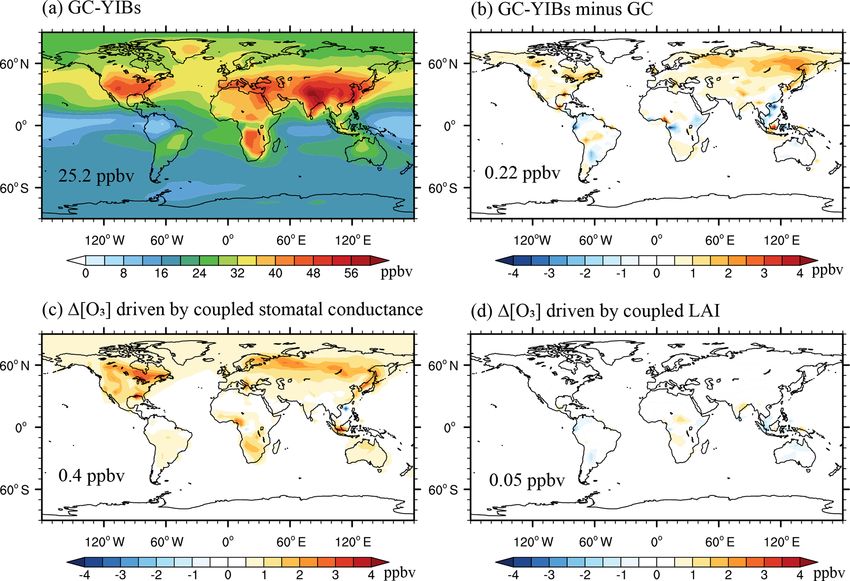
1138                                                               Y. Lei et al.: A tool for biosphere–chemistry interactions

counts for ∼ 25 % of the total O3 removed from the tropo-          php/GEOS-Chem_12#12.0.0, last access: 10 January 2020).
sphere (Lelieveld and Dentener, 2000).                             The GEOS-Chem (GC) model has been widely used in
    In turn, atmospheric chemistry can also affect the terres-     episode prediction (Cui et al., 2016), source attribution
trial biosphere (McGrath et al., 2015; Schiferl and Heald,         (D’Andrea et al., 2016; Dunker et al., 2017; Ni et al., 2018;
2018; Yue and Unger, 2018). Surface O3 has a negative im-          Lu et al., 2019), future pollution projection (Yue et al., 2015;
pact on plant photosynthesis and crop yields by reducing gas       Ramnarine et al., 2019), health risk assessment (Xie et al.,
exchange and inducing phytotoxic damage to plant tissues           2019), and so on. The standard GC model uses prescribed
(Van Dingenen et al., 2009; Wilkinson et al., 2012; Yue and        vegetation parameters and as a result cannot depict the
Unger, 2014). Unlike O3 , the effect of aerosols on vegeta-        changes in chemical components due to biosphere–pollution
tion is dependent on the aerosol concentrations. Moderate          interactions. The updated GC-YIBs model links atmospheric
increase of aerosols in the atmosphere is beneficial to veg-       chemistry with biosphere in a two-way coupling such that
etation (Mahowald, 2011; Schiferl and Heald, 2018). The            changes in chemical components or vegetation will simulta-
aerosol-induced enhancement in diffuse light results in more       neously feed back to influence the other systems. Here, we
radiation reaching surface from all directions than solely         evaluate the dynamically simulated dry deposition and leaf
from above. As a result, leaves in the shade or at the bottom      area index (LAI) from GC-YIBs and examine the consequent
of the canopy can receive more radiation and are able to as-       impacts on surface O3 . We also quantify the detrimental ef-
similate more CO2 through photosynthesis, leading to an in-        fects of O3 on gross primary productivity (GPP) using instant
crease of canopy productivity (Mercado et al., 2009; Yue and       pollution concentrations from the chemical module. For the
Unger, 2018). However, excessive aerosol loadings reduce           first step, we focus on the coupling between O3 and vegeta-
canopy productivity because the total radiation is largely         tion. The interactions between aerosols and vegetation will
weakened (Alton, 2008; Yue and Unger, 2017).                       be developed and evaluated in the future. The next section
    Models are essential tools to understand and quantify          describes the GC-YIBs model and the evaluation data. Sec-
the interactions between the terrestrial biosphere and at-         tion 3 compares simulated O3 from GC-YIBs with that from
mospheric chemistry at the global and/or regional scales.          the original GC models and explores the causes of differ-
Many studies have performed multiple global simulations            ences. Section 4 quantifies the damaging effects of O3 on
with climate–chemistry–biosphere models to quantify the ef-        global GPP using the GC-YIBs model. The last section sum-
fects of air pollutants on the terrestrial biosphere (Mercado et   marizes progress and discusses the next steps in optimizing
al., 2009; Yue and Unger, 2015; Oliver et al., 2018; Schiferl      the GC-YIBs model.
and Heald, 2018). In contrast, very few studies have quan-
tified the O3 -induced biogeochemical and meteorological
feedbacks to air pollution concentrations (Sadiq et al., 2017;     2     Methods and data
Zhou et al., 2018). Although considerable efforts have been
made, uncertainties in biosphere–chemistry interactions re-        2.1    Descriptions of the YIBs model
main large because their two-way coupling is not adequately
represented in the current generation of terrestrial biosphere     YIBs is a terrestrial vegetation model designed to simulate
models or global chemistry models. Global terrestrial bio-         the land carbon cycle with dynamical prediction of LAI and
sphere models usually use prescribed O3 and aerosol con-           tree height (Yue and Unger, 2015). The YIBs model applies
centrations (Sitch et al., 2007; Mercado et al., 2009; Lombar-     the Farquhar et al. (1980) scheme to calculate leaf level pho-
dozzi et al., 2012), and global chemistry models often apply       tosynthesis, which is further upscaled to the canopy level by
fixed offline vegetation variables (Lamarque et al., 2013). For    the separation of sunlit and shaded leaves (Spitters, 1986).
example, stomatal conductance, which plays a crucial role          The canopy is divided into an adaptive number of layers (typ-
in regulating the water cycle and altering pollution deposi-       ically 2–16) for light stratification. Sunlight is attenuated and
tion, responds dynamically to vegetation biophysics and en-        becomes more diffusive when penetrating the canopy. The
vironmental stressors at various spatiotemporal scales (Het-       sunlit leaves can receive both direct and diffuse radiation,
herington and Woodward, 2003; Franks et al., 2017). How-           while the shaded leaves receive only diffuse radiation. The
ever, these processes are either missing or lack temporal vari-    leaf-level photosynthesis, calculated as the sum of sunlit and
ations in most current chemical transport models (Verbeke et       shaded leaves, is then integrated over all canopy layers to de-
al., 2015). The fully two-way coupling between biosphere           rive the GPP of ecosystems.
and chemistry is necessary to better quantify the responses           The model considers nine plant functional types (PFTs),
of ecosystems and pollution to global changes.                     including evergreen needleleaf forest, deciduous broadleaf
    In this study, we develop the GC-YIBs model by                 forest, evergreen broadleaf forest, shrubland, tundra, C3 and
implementing the Yale Interactive terrestrial Biosphere            C4 grasses, and C3 and C4 crops. The satellite-based land
(YIBs) model version 1.0 (Yue and Unger, 2015) into                types and cover fraction are aggregated into these nine PFTs
the chemical transport model (CTM) GEOS-Chem ver-                  and used as input (Fig. S1 in the Supplement). The initial soil
sion 12.0.0 (http://wiki.seas.harvard.edu/geos-chem/index.         carbon pool and tree height used in YIBs are from the 140-

Geosci. Model Dev., 13, 1137–1153, 2020                                              www.geosci-model-dev.net/13/1137/2020/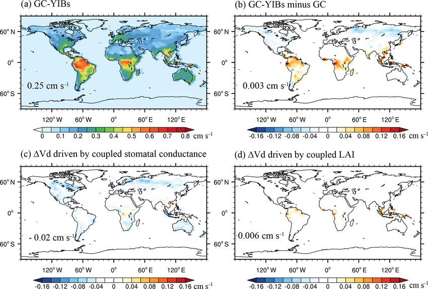
Y. Lei et al.: A tool for biosphere–chemistry interactions 1139
year spin-up processes (Yue and Unger, 2015). The YIBs is tent Cveg is updated every 10 days:
driven with hourly 2-D meteorology and 3-D soil variables
(six layers) from the Modern-Era Retrospective analysis for dCveg
= (1 − τ ) × NPP − ϕ, (6)
Research and Applications, version 2 (MERRA2). dt
The YIBs uses the model of Ball and Berry (Baldocchi et
where τ and ϕ represent partitioning parameter and litter fall
al., 1987) to compute leaf stomatal conductance:
rate, respectively; their calculation methods have been doc-
1 Anet umented in Yue and Unger (2015). Net primary productivity
gs = =m RH + b, (1) (NPP) is calculated as the residue of subtracting autotrophic
rs cs
respiration (Ra ) from GPP:
where rs is the leaf stomatal resistance (s m−1 ); m is the em-
pirical slope of the Ball–Berry stomatal conductance equa- NPP = GPP − Ra . (7)
tion and is affected by water stress; cs is the CO2 concen-
tration at the leaf surface (µmol m−3 ); RH is the relative In addition, the YIBs model implements the scheme for
humidity of the atmosphere; b (m s−1 ) represents the mini- O3 damage on vegetation proposed by Sitch et al. (2007).
mum leaf stomatal conductance when net leaf photosynthe- The scheme directly modifies photosynthesis using a semi-
sis (Anet , µmol m−2 s−1 ) is 0. For different PFTs, appropriate mechanistic parameterization, which in turn affects stom-
photosynthetic parameters are derived from the Community atal conductance. The O3 damage factor is considered as the
Land Model (CLM; Bonan et al., 2011). function of stomatal O3 flux:
The net leaf photosynthesis for C3 and C4 plants is com-
puted based on well-established Michaelis–Menten enzyme- −a FO3 − TO3 , FO3 > TO3
F= , (8)
kinetics scheme (Farquhar et al., 1980; von Caemmerer and 0, FO3 ≤ TO3
Farquhar, 1981): where a represents the sensitivity to damage and TO3 repre-
Anet = min (Jc , Je , Js ) − Rd , (2) sents the O3 flux threshold (µmol m−2 s−1 ). For a specific
PFT, the values of coefficient a vary from low to high to
where Jc , Je , and Js represent Rubisco-limited photosynthe- represent a range of uncertainties for ozone vegetation dam-
sis, RuBP-limited photosynthesis, and product-limited pho- age (Table S1 in the Supplement). TO3 is a critical threshold
tosynthesis, respectively. Rd is the rate of dark respiration. for O3 damage and varies with PFTs. The F becomes neg-
They are all parameterized as functions of the maximum car- ative only if FO3 is higher than TO3 . Stomatal O3 flux FO3
boxylation capacity (Collatz et al., 1991) and meteorological (µmol m−2 s−1 ) is calculated as follows:
variables (e.g., temperature, radiation, and CO2 concentra-
tions). [O3 ]
FO3 = , (9)
The YIBs model applies the LAI and carbon allocation ra + rb + k · rs
schemes from the TRIFFID model (Cox, 2001; Clark et al.,
where [O3 ] represents O3 concentrations at top of the canopy
2011). On the daily scale, canopy LAI is calculated as fol-
(µmol m−3 ); ra is aerodynamic resistance (s m−1 ); rb is
lows:
boundary layer resistance (s m−1 ); rs represents stomatal re-
LAI = f × LAImax , (3) sistance (s m−1 ). The Sitch et al. (2007) scheme within the
YIBs framework has been well evaluated against hundreds
where f represents the phenological factor controlled by me- of observations globally (Yue and Unger, 2018) and region-
teorological variables (e.g., temperature, water availability, ally Yue et al., 2016, 2017).
and photoperiod); LAImax represents the available maximum
LAI related to tree height, which is dependent on the vegeta- 2.2 Descriptions of the GEOS-Chem model
tion carbon content (Cveg ). The Cveg is calculated as follows:
GC is a global 3-D model of atmospheric compositions
Cveg = Cl + Cr + Cw , (4) with fully coupled O3 –NOx –hydrocarbon–aerosol chemical
mechanisms (Gantt et al., 2015; Lee et al., 2017; Ni et al.,
where Cl , Cr , and Cw represent leaf, root, and stem carbon 2018). In this study, we use GC version 12.0.0 driven by as-
contents, respectively. And all carbon components are pa- similated meteorology from MERRA2 with a horizontal res-
rameterized as the function of LAImax : olution of 4◦ latitude by 5◦ longitude and 47 vertical layers
Cl = α × LAI from the surface to 0.01 hPa.
Cr = α × LAImax , (5) In GC, terrestrial vegetation modulates tropospheric O3
Cr = β × LAImax
γ mainly through LAI and canopy stomatal conductance,
which affect both the sources and sinks of tropospheric O3
where α represents the specific leaf carbon density; β and γ through changes in BVOC emissions, soil NOx emissions,
represent allometric parameters. The vegetation carbon con- and dry deposition (Zhou et al., 2018). BVOC emissions are
www.geosci-model-dev.net/13/1137/2020/ Geosci. Model Dev., 13, 1137–1153, 2020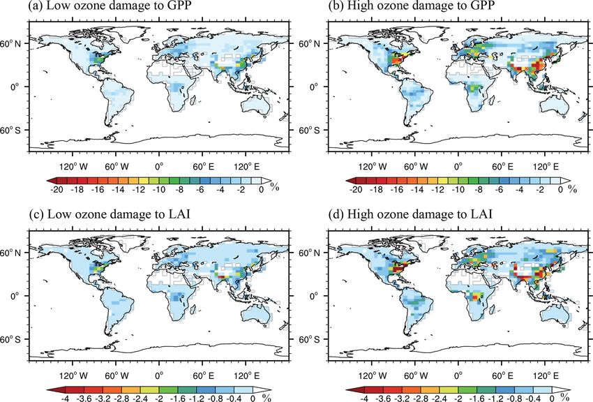
1140 Y. Lei et al.: A tool for biosphere–chemistry interactions
Table 1. Summary of simulations using the GC-YIBs model.
Name Scheme Ozone effects
monthly prescribed MODIS LAI
Offline no
original dry deposition scheme
daily dynamically predicted LAI
Online_LAI no
original dry deposition scheme
monthly prescribed MODIS LAI
Online_GS no
hourly predicted stomatal conductance
daily dynamically predicted LAI
Online_ALL no
hourly predicted stomatal conductance
daily dynamically predicted LAI
Online_ALL_HS hourly predicted stomatal conductance high
hourly predicted [O3 ] by GC model
daily dynamically predicted LAI
Online_ALL_LS hourly predicted stomatal conductance low
hourly predicted [O3 ] by GC model
where Ra (m s−1 ) is the aerodynamic resistance represent-
ing the ability of the airflow to bring gases or particles close
to the surface and is dependent mainly on the atmospheric
turbulence structure and the height considered. Rb (m s−1 )
is the boundary resistance driven by the characteristics of
the surface (surface roughness) and gas/particle (molecular
diffusivity). Ra and Rb are calculated from the meteorologi-
cal variables of global climate models (GCMs; Jacob et al.,
1992). The surface resistance Rc is determined by the affin-
ity of the surface for the chemical compound. For O3 over
vegetated regions, Vd is mainly driven by Rc (m s−1 ) during
the daytime because the effects of Ra and Rb are generally
small. Surface resistances Rc are computed using the We-
sely (1989) canopy model with some improvements, includ-
ing explicit dependence of canopy stomatal resistances on
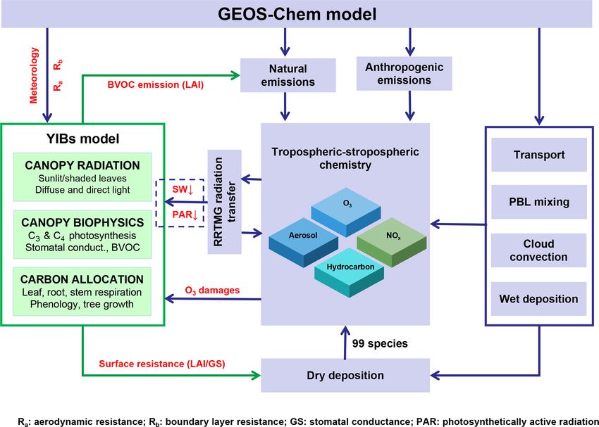
Figure 1. Diagram of the GC-YIBs global carbon-chemistry model. LAI (Gao and Wesely, 1995) and direct/diffuse PAR within
Processes with red font are implemented in this study. Processes in the canopy (Baldocchi et al., 1987):
the blue dashed box will be developed in the future.
1 1 1 1 1
= + + + , (11)
Rc Rs + Rm Rlu Rcl Rg
calculated based on a baseline emission factor parameterized where Rs is the stomatal resistance (s m−1 ), Rm is the leaf
as the function of light, temperature, leaf age, soil moisture, mesophyll resistance (Rm = 0 s m−1 for O3 ), Rlu is the upper
LAI, and CO2 inhibition within the Model of Emissions of canopy or leaf cuticle resistance, and Rcl is the lower canopy
Gases and Aerosols from Nature (MEGAN v2.1; Guenther resistance (s m−1 ). Rs is calculated based on minimum stom-
et al., 2006). Soil NOx emission is computed based on the atal resistance (rs , s m−1 ), solar radiation (G, W m−2 ), sur-
scheme of Hudman et al. (2012) and further modulated by a face air temperature (Ts , ◦ C), and the molecular diffusivities
reduction factor to account for within-canopy NOx deposi- (DH2 O and Dx ) for a specific gas x:
tion (Rogers and Whitman, 1991). The dry deposition veloc-
1 400 DH2 O
ity (Vd , m s−1 ) for O3 is computed based on a resistance-in- Rs = rs 1 + . (12)
2 T (40 − T ) Dx
series model within GC: [200 (G + 0.1)] s s
In GC, the above parameters related to Rc have prescribed
1 values for 11 deposition land types: snow/ice, deciduous
Vd = , (10) forest, coniferous forest, agricultural land, shrub/grassland,
Ra + Rb + Rc
Geosci. Model Dev., 13, 1137–1153, 2020 www.geosci-model-dev.net/13/1137/2020/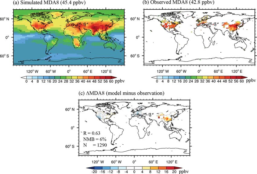
Y. Lei et al.: A tool for biosphere–chemistry interactions                                                                      1141

Table 2. List of measurement sites used for dry deposition evaluation.

                                                                                   Daytime
                    Land type            Longitude     Latitude    Season      Vd (cm s−1 )     References
                                                                   summer             0.92
                                         80.9◦ W       44.3◦ N                                  Padro et al. (1991)
                                                                   winter             0.28
                                                                   summer             0.61
                                         72.2◦ W       42.7◦ N                                  Munger et al. (1996)
                                                                   winter             0.28
                    Deciduous forest     75.2◦ W       43.6◦ N     summer             0.82
                                                                                                Finkelstein et al. (2000)
                                         78.8◦ W       41.6◦ N     summer             0.83
                                                                   spring             0.38
                                         99.7◦ E       18.3◦ N                                  Matsuda et al. (2005)
                                                                   summer             0.65
                                         0.84◦ W       51.17◦ N    Jul–Aug            0.85      Fowler et al. (2009)
                                         0.7◦ W        44.2◦ N     Jun                0.62      Lamarque et al. (2013)
                                         79.56◦ W      44.19◦ N    summer             0.91      Wu et al. (2016)
                                         61.8◦ W       10.1◦ S     wet                 1.1      Rummel et al. (2007)
                    Amazon forest
                                         117.9◦ E      4.9◦ N      wet                 1.0      Fowler et al. (2011)
                                         3.4◦ W        55.3◦ N     spring             0.58      Coe et al. (1995)
                                         66.7◦ W       54.8◦ N     summer             0.26      Munger et al. (1996)
                                                                   spring             0.31
                                                                   summer             0.48
                                         11.1◦ E       60.4◦ N                                  Hole et al. (2004)
                                                                   autumn               0.2
                                                                   winter            0.074
                    Coniferous forest
                                                                   spring             0.68
                                         8.4◦ E        56.3◦ N     summer              0.8      Mikkelsen et al. (2004)
                                                                   autumn             0.83
                                         18.53◦ E      49.55◦ N    Jul–Aug             0.5      Zapletal et al. (2011)
                                         79.1◦ W       36◦ N       spring             0.79      Finkelstein et al. (2000)
                                         120.6◦ W      38.9◦ N     summer             0.59      Kurpius et al. (2002)
                                         0.7◦ W        44.2◦ N     summer             0.48      Lamaud et al. (1994)
                                         105.5◦ E      40◦ N       summer             0.39      Turnipseed et al. (2009)

Amazon forest, tundra, desert, wetland, urban and water                  2.3   Implementation of YIBs into GEOS-Chem
(Wesely, 1989; Jacob et al., 1992).                                            (GC-YIBs)
   Although the stomatal conductance scheme of We-
sely (1989) has been widely used in chemical transport and
climate models, considerable limits still exist because this             In this study, GC model time steps are set to 30 min for
scheme does not consider the response of stomatal conduc-                transport and convection and 60 min for emissions and chem-
tance to phenology, CO2 concentrations, or soil water avail-             istry. In the online GC-YIBs configuration, GC provides the
ability (Rydsaa et al., 2016; Lin et al., 2017). Previous stud-          hourly meteorology, aerodynamic resistance, boundary layer
ies have well evaluated the dry deposition scheme used in                resistance, and surface [O3 ] to YIBs. Without YIBs imple-
the GEOS-Chem model against observations globally and re-                mentation, the GC model computes O3 dry deposition ve-
gionally (Hardacre et al., 2015; Silva and Heald, 2018; Lin et           locity using prescribed LAI and parameterized canopy stom-
al., 2019; Wong et al., 2019). They found that GEOS-Chem                 atal resistance (Rs ), and as a result ignores feedbacks from
can generally capture the diurnal and seasonal cycles except             ecosystems (details in Sect. 2.2). With YIBs embedded, daily
for the amplitude of O3 dry deposition velocity (Silva and               LAI and hourly stomatal conductance are dynamically pre-
Heald, 2018).                                                            dicted for the dry deposition scheme within the GC model.
                                                                         The online-simulated surface [O3 ] affects carbon assimila-
                                                                         tion and canopy stomatal conductance; in turn, the online-
                                                                         simulated vegetation variables such as LAI and stomatal con-
                                                                         ductance affect both the sources and sinks of O3 by altering

www.geosci-model-dev.net/13/1137/2020/                                                        Geosci. Model Dev., 13, 1137–1153, 2020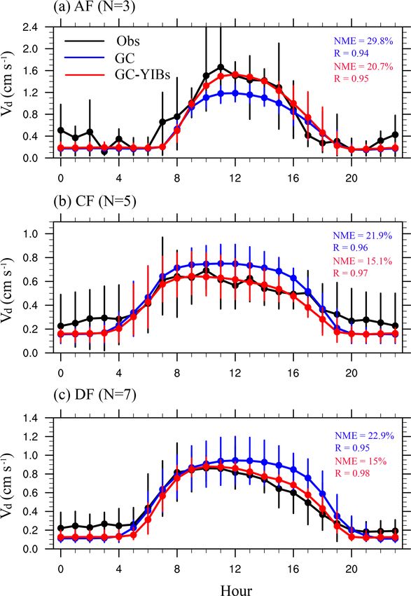
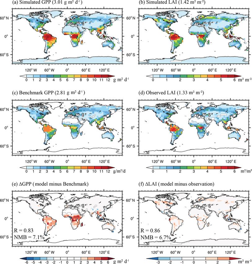
1142                                                                    Y. Lei et al.: A tool for biosphere–chemistry interactions

Figure 2. Annual gross primary productivity (GPP) and leaf area index (LAI) from offline simulations (a, b), observations (c, d), and their
differences (e, f) averaged for the period of 2010–2012. Global area-weighted GPP and LAI are shown in parentheses in the panel captions.
The correlation coefficients (R) and global normalized mean biases (NMBs) are shown in the bottom panels.

precursor emissions and dry deposition at the 1 h integration           ters. At specific grids (4◦ × 5◦ or 2◦ × 2.5◦ ), dry deposition
time step. The above processes are summarized in Fig. 1.                velocity is calculated as the weighted sum of native reso-
   To retain the corresponding relationship between vegeta-             lution (0.25◦ × 0.25◦ ). Replacing of Olson with YIBs land
tion parameters and land cover map in the GC-YIBs model,                types induces a global mean difference of −0.59 ppbv on sur-
we replace the Olson 2001 land cover map in GC with                     face [O3 ] (Fig. S3). Large discrepancies are found in Africa
satellite-retrieved land cover dataset used by YIBs (Defries et         and the southern Amazon, where the local [O3 ] decreases by
al., 2000; Hanninen and Kramer, 2007). The conversion re-               more than 2 ppbv with the new land types. However, limited
lationships between YIBs land types and GC deposition land              differences are shown in the middle-to-high latitudes of the
types are summarized in Table S2. The global spatial pattern            Northern Hemisphere (NH, Fig. S3).
of deposition land types converted from YIBs land types is
shown in Fig. S2. The Olson 2001 land cover map used in                 2.4   Model simulations
GC version 12.0.0 has a native resolution of 0.25◦ × 0.25◦
and 74 land types (Olson et al., 2001). Each of the Olson               We conduct six simulations to evaluate the performance of
land types is associated with a corresponding deposition land           GC-YIBs and to quantify global O3 damage to vegetation
type with prescribed parameters. There are 74 Olson land                (Table 1): (i) Offline, a control run using the offline GC-
types but only 11 deposition land types, suggesting that many           YIBs model. The YIBs module shares the same meteorolog-
of the Olson land types share the same deposition parame-               ical forcing as the GC module and predicts both GPP and

Geosci. Model Dev., 13, 1137–1153, 2020                                                    www.geosci-model-dev.net/13/1137/2020/
Y. Lei et al.: A tool for biosphere–chemistry interactions                                                                         1143

Figure 3. Annual surface O3 concentrations ([O3 ]) from offline simulations (a), observations (b), and their differences (c) averaged for
the period of 2010–2012. Global area-weighted surface [O3 ] over grids with available observations are shown in parentheses in the panel
captions. The correlation coefficient (R) and global normalized mean biases (NMBs) are shown in the bottom panel with indication of grid
numbers (N ) used for statistics.

Figure 4. Simulated annual surface [O3 ] from online GC-YIBs model (a) and its changes (b–d) relative to offline simulations. Changes
of [O3 ] are caused by (b) jointly coupled LAI and stomatal conductance (Online_ALL – Offline), (c) coupled stomatal conductance alone
(Online_ALL – Online_LAI), and (d) coupled LAI alone (Online_ALL – Online_GS). Global area-weighted [O3 ] or 1 [O3 ] are shown in
the panels.

www.geosci-model-dev.net/13/1137/2020/                                                    Geosci. Model Dev., 13, 1137–1153, 2020
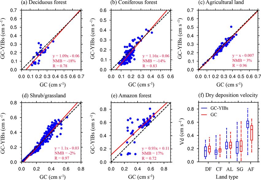
1144                                                                        Y. Lei et al.: A tool for biosphere–chemistry interactions

Figure 5. Simulated annual O3 dry deposition velocity from online GC-YIBs model (a) and its changes caused by coupled LAI and stomatal
conductance (b–d) averaged for the period of 2010–2012. The changes of dry deposition velocity are driven by (b) coupled LAI and stomatal
conductance (Online_ALL – Offline), (c) coupled stomatal conductance alone (Online_ALL – Online_LAI), and (d) coupled LAI alone
(Online_ALL – Online_GS). Global area-weighted annual O3 dry deposition velocity and changes are shown in the panels.

Figure 6. Comparisons of annual O3 dry deposition velocity between online GC-YIBs (Online_ALL simulation) and GC (Offline simulation)
models for different land types, including (a) deciduous forest (DF), (b) coniferous forest (CF), (c) agricultural land (AL), (d) shrub/grassland
(SG), and (e) Amazon forest (AF). The box plots of dry deposition velocity simulated by online GC-YIBs (blue) and GC models (red) for
different land types are shown in (f). Each point in (a–e) represents annual O3 dry deposition velocity at one grid point averaged for the period
of 2010–2012. The red lines indicate linear regressions between predictions from GC-YIBs and GC models. The regression fit, correlation
coefficient (R), and normalized mean biases (NMBs) are shown in each panel.

Geosci. Model Dev., 13, 1137–1153, 2020                                                        www.geosci-model-dev.net/13/1137/2020/
Y. Lei et al.: A tool for biosphere–chemistry interactions 1145
stomatal conductance. The last three runs are used to quan-
tify the global O3 damage on ecosystem productivity.
2.5 Evaluation data
We use observed LAI data for 2010–2012 from the MODIS
product. Benchmark GPP product of 2010–2012 is estimated
by upscaling ground-based FLUXNET eddy covariance data
using a model tree ensemble approach, a type of machine
learning technique (Jung et al., 2009). Although these prod-
ucts may have certain biases, they have been widely used
to evaluate land surface models because direct observations
of GPP and LAI are not available on the global scale (Yue
and Unger, 2015; Slevin et al., 2017; Swart et al., 2019).
Measurements of surface [O3 ] over North America and Eu-
rope are provided by the global gridded surface ozone data
set of Sofen et al. (2016), and those over China are interpo-
lated from data at ∼ 1500 sites operated by China’s Ministry
of Ecology and Environment (http://www.cnemc.cn/en/, last
access: 10 January 2020). We perform literature research to
collect data of dry deposition velocity from eight deciduous
forest, two Amazon forest, and nine coniferous forest sites
(Table 2).
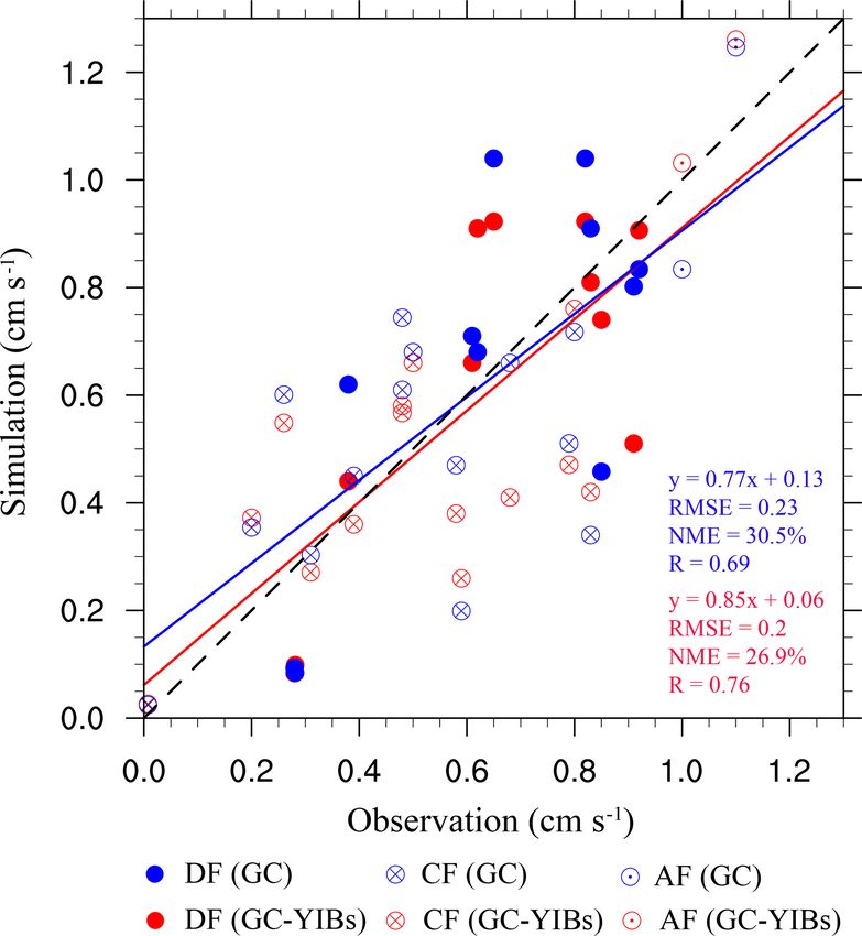
Figure 7. Comparison between observed and simulated O3 dry de-
position velocity at the observational sites. The different marker
types represent different land types. The blue and red markers rep- 3 Results
resent the simulation results from online GC-YIBs (Online_ALL
simulation) and GC (Offline simulation) models, respectively. The 3.1 Evaluation of the offline GC-YIBs model
blue and red lines indicate linear regressions between simulations
and observations. The regression fits, root-mean-square errors (RM- With the offline simulation, the simulated GPP and LAI are
SEs), normalized mean errors (NMEs), and correlation coefficients compared with observed LAI and benchmark GPP for the
(R) for GC-YIBs (blue) and GC (red) models are also shown. period of 2010–2012 (Fig. 2). Observed LAI and benchmark
GPP both show high values in the tropics and medium values
in the northern middle-to-high latitudes. Compared to ob-
servations, the GC-YIBs model forced with MERRA2 me-
LAI. However, predicted vegetation variables are not fed into teorology depicts similar spatial distributions, with spatial
GC, which is instead driven by prescribed LAI from Moder- correlation coefficients of 0.83 (p < 0.01) for GPP and 0.86
ate Resolution Imaging Spectroradiometer (MODIS) product (p < 0.01) for LAI. Although the model overestimates LAI
and parameterized canopy stomatal conductance proposed by in the tropics and northern high latitudes by 1–2 m2 m−2 , the
Gao and Wesely (1995). (ii) Online_LAI is a sensitive run us- simulated global area-weighted LAI (1.42 m2 m−2 ) is close
ing online GC-YIBs with dynamically predicted daily LAI to observations (1.33 m2 m−2 ), with a normalized mean bias
from YIBs but prescribed stomatal conductance. (iii) On- (NMB) of 6.7 %. Similar to LAI, the global NMB for GPP is
line_GS is another sensitive run using YIBs-predicted stom- only 7.1 %, though there are substantial regional biases, espe-
atal conductance but prescribed MODIS LAI. (iv) In On- cially in the Amazon and central Africa. Such differences are
line_ALL, both YIBs-predicted LAI and stomatal conduc- in part attributed to the underestimation of GPP for tropical
tance are used for GC. (v) Online_ALL_HS is the same as rainforests in the benchmark product, because the recent sim-
Online_ALL except it predicts surface O3 damage to plant ulations at eight rainforest sites with YIBs model reproduced
photosynthesis with high sensitivities. (vi) Online_ALL_ LS ground-based observations well (Yue and Unger, 2018).
is the same as Online_ALL_HS but with low O3 damage sen- We then evaluate simulated annual mean surface [O3 ] dur-
sitivities. Each simulation is run from 2006 to 2012 with the ing 2010–2012 based on an offline simulation (Fig. 3). The
first 4 years for spin up, and the results from 2010 to 2012 simulated high values are mainly located in the mid-latitudes
are used to evaluate the online GC-YIBs model. The differ- of NH (Fig. 3a). Compared to observations, simulations show
ences between Online_ALL and Online_GS (Online_LAI) reasonable spatial distribution with a correlation coefficient
represent the effects of coupled LAI (stomatal conductance) of 0.63 (p < 0.01). Although the offline GC-YIBs model
on simulated [O3 ]. Differences between Offline and On- overestimates annual [O3 ] in southern China and predicts
line_ALL then represent joint effects of coupled LAI and lower values in western Europe and western USA, the sim-
www.geosci-model-dev.net/13/1137/2020/ Geosci. Model Dev., 13, 1137–1153, 2020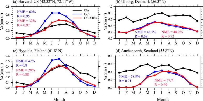
1146                                                                   Y. Lei et al.: A tool for biosphere–chemistry interactions

Figure 8. Comparison of monthly O3 dry deposition velocity at the Harvard (a), Ulborg (b), Hyytiälä (c), and Auchencorth (d) sites. The
black lines represent observed O3 dry deposition velocity. The blue and red lines represent simulated O3 dry deposition velocity from GC
(Offline simulation) and online GC-YIBs (Online_ALL simulation) models, respectively.

ulated area-weighted surface [O3 ] (45.4 ppbv) is only 6 %            ferent sensitivity experiments. The global average velocity
higher than observations (42.8 ppbv). Predicted summertime            is 0.25 cm s−1 with a regional maximum of 0.5–0.7 cm s−1
surface [O3 ] instead shows positive biases in eastern USA            in tropical rainforests (Fig. 5a), especially over the Ama-
and Europe (Fig. S4), consistent with previous evaluations            zon and central Africa, where high ecosystem productivity
using the GC model (Travis et al., 2016; Schiferl and Heald,          is observed (Fig. 2). With implementation of YIBs into GC,
2018; Yue and Unger, 2018).                                           simulated dry deposition velocity increases over tropical re-
                                                                      gions but decreases in the middle-to-high latitudes of NH
3.2    Changes of surface O3 in the online GC-YIBs                    (Fig. 5b). Larger dry deposition results in lower [O3 ] in the
       model                                                          tropics, while smaller dry deposition increases [O3 ] in boreal
                                                                      regions. Such spatial patterns are broadly consistent with 1
Surface O3 is changed by the coupling of LAI and stomatal             [O3 ] in online GC-YIBs (Fig. 4b). In a comparison, updated
conductance (Fig. 4). Global [O3 ] shows similar patterns be-         LAI induces limited changes in the isoprene and NOx emis-
tween Offline (Fig. 3a) and Online_ALL (Fig. 4a) simula-              sions (Fig. S5), suggesting that changes of dry deposition
tions. However, the online GC-YIBs predicts [O3 ] of 0.5–             velocity are the dominant drivers of O3 changes. Both the
2 ppbv higher in the middle-to-high latitudes of NH, lead-            updated LAI and stomatal conductance influence dry depo-
ing to an average [O3 ] enhancement of 0.22 ppbv compared             sition. Sensitivity experiments further show that changes in
to offline simulations (Fig. 4b). Regionally, some negative           dry deposition are mainly driven by coupled canopy stom-
changes of 1–2 ppbv can be found at the tropical regions.             atal conductance (Fig. 5c) instead of LAI (Fig. 5d), though
With sensitivity experiments Online_LAI and Online_GS                 the latter contributes to the enhanced dry deposition in the
(Table 1), we separate the contributions of LAI and stom-             tropics.
atal conductance changes to 1 [O3 ]. It is found that 1 [O3 ]            The original GC dry deposition scheme applies fixed pa-
between Online_ALL and Online_LAI (Fig. 4c) resembles                 rameters for stomatal conductance of a specific land type.
the total 1 [O3 ] pattern (Fig. 4b), suggesting that changes          The updated GC-YIBs model instead calculates stomatal
in stomatal conductance play the dominant role in regulat-            conductance as a function of photosynthesis and environ-
ing surface [O3 ]. As a comparison, 1 [O3 ] values between            mental forcings (Eq. 1). As a result, predicted dry deposition
Online_ALL and Online_GS show limited changes glob-                   exhibits discrepancies among biomes. With Offline and On-
ally (by 0.05 ppbv) and moderate changes in tropical regions          line_ALL simulations, we further evaluate the performance
(Fig. 4d), mainly because the LAI predicted by YIBs is close          of online GC-YIBs in simulating O3 dry deposition velocity
to MODIS LAI used in GC (Fig. 2). It is noticed that the av-          for specific deposition land types (Fig. 6). For agricultural
erage 1 [O3 ] in Fig. 4b is not equal to the sum of Fig. 4c           land and shrub/grassland, the simulated O3 dry deposition
and d, because of the non-linear effects.                             velocity for online GC-YIBs model is close to the GC model,
   We further explore the possible causes of differences in           with NMBs of 3 % and −2 % and correlation coefficients
simulated [O3 ] between online and offline GC-YIBs models.            of 0.96 and 0.97, respectively. However, the simulated dry
Figure 5 shows simulated annual O3 dry deposition veloc-              deposition velocity in online GC-YIBs is lower than GC by
ity from the online GC-YIBs model and its changes in dif-             18 % for deciduous forests and 14 % for coniferous forests,

Geosci. Model Dev., 13, 1137–1153, 2020                                                  www.geosci-model-dev.net/13/1137/2020/
Y. Lei et al.: A tool for biosphere–chemistry interactions 1147
prediction at the other Amazon forest site. Overall, the sim-
ulated daytime O3 dry deposition velocities in online GC-
YIBs model are closer to observations than those in the GC
model with smaller NME (26.9 % vs. 30.5 %), root-mean-
square errors (RMSEs, 0.2 vs. 0.23) and higher correlation
coefficients (0.76 vs. 0.69). Such improvements consolidate
our strategies in updating GC model to the fully coupled GC-
YIBs model.
We collect long-term measurements from four sites across
North America and western Europe to evaluate the model
performance in simulating seasonal cycle of O3 dry depo-
sition velocity (Fig. 8). The GC model well captures the
seasonal cycles of O3 dry deposition velocity in all sites
with the correlation coefficients of 0.95 at Harvard, 0.8 at
Hyytiälä, 0.68 at Ulborg, and 0.71 at Auchencorth. How-
ever, the magnitude of O3 dry deposition velocity is over-
estimated at the Harvard and Hyytiälä sites (NME of 60 %
and 42 %, respectively), but underestimated at the Ulborg
and Auchencorth sites (NME of 48.7 % and 58.9 %, respec-
tively) at growing seasons. Compared to the GC model, sim-
ulated O3 dry deposition velocity with the GC-YIBs model
shows large improvements over Harvard (Hyytiälä), where
the model-to-observation NME decreases from 60 % (42 %)
to 32 % (28 %).
Additionally, we investigate the diurnal cycle of O3 dry
deposition velocity at 15 sites (Fig. S6). Observed O3 dry de-
position velocities show a single diurnal peak with the max-
imum from 08:00 to 16:00 local time (Fig. 9). Compared to
observations, the GC model has good performance in simu-
lating the diurnal cycle with correlation coefficients of 0.94
Figure 9. Comparison of multi-site mean diurnal cycle of O3 dry
deposition velocity at the Amazon (a), coniferous (b), and decidu-
for Amazon forests, 0.96 for coniferous forests, and 0.95
ous (c) forests. Error bars represent the range of values from differ- for deciduous forests. The GC model underestimates day-
ent sites. Black lines represent observed O3 dry deposition velocity. time O3 dry deposition velocity for Amazon forests (NME
The blue and red lines represent simulated O3 dry deposition veloc- of 29.8 %) but overestimates it for coniferous and deciduous
ity by GC (Offline simulation) and online GC-YIBs (Online_ALL forests (NME of 21.9 % and 22.9 %, respectively). Compared
simulation) models, respectively. The site number (N), R, and NME to the GC model, the simulated daytime O3 dry deposition
are shown for each panel. velocities using the GC-YIBs model are closer to observa-
tions in all three biomes. The NMEs decrease by 9.1 % for
Amazon forests, 6.8 % for coniferous forests, and 7.9 % for
but larger by 17 % for Amazon forests. Such changes match deciduous forests.
the spatial pattern of dry deposition shown in Fig. 5b.
Since the changes of O3 dry deposition velocity are mainly 3.3 Assessment of global O3 damage to vegetation
found in deciduous forests, coniferous forests, and Amazon
forests, we collect 27 samples across these three biomes An important feature of GC-YIBs is the inclusion of on-
to evaluate the online GC-YIBs model (Table 2). For the line vegetation damage by surface O3 . Here, we quantify
11 samples in deciduous forests, the normalized mean er- the global O3 damage to GPP and LAI by conducting On-
ror (NME) decreases from 29 % in the GC model to 24 % line_ALL_HS and Online_ALL_LS simulations (Fig. 10).
in GC-YIBs with lower relative errors at eight sites (Fig. 7). Due to O3 damage, annual GPP declines from −1.5 % (low
Predictions with the GC-YIBs also show large improvements sensitivity) to −3.6 % (high sensitivity) on the global scale.
over coniferous forests, where 8 out of 14 samples show Regionally, O3 decreases GPP by as much as 10.9 % in the
lower (decreases from 27 % in GC to 25 % in GC-YIBs) eastern USA and up to 14.1 % in eastern China at high sensi-
errors. For Amazon forests, the GC-YIBs model signifi- tivity (Fig. 10a, b). Such strong damage is related to (i) high
cantly improves the prediction at one site (117.9◦ E, 4.9◦ N), ambient [O3 ] due to anthropogenic emissions and (ii) large
where the original error of −0.17 cm s−1 is limited to only stomatal conductance due to active ecosystem productivity in
0.03 cm s−1 . However, the new model does not improve the monsoon areas. The O3 effects are moderate in tropical areas,
www.geosci-model-dev.net/13/1137/2020/ Geosci. Model Dev., 13, 1137–1153, 20201148 Y. Lei et al.: A tool for biosphere–chemistry interactions
Figure 10. Percentage changes in (a, b) GPP and (c, d) LAI caused by the damaging effects of O3 with (a, c) low (Online_ALL_LS
simulation) and (b, d) high sensitivities (Online_ALL_HS simulation). Both changes of GPP and LAI are averaged for 2010–2012.
where stomatal conductance is also high, while [O3 ] is very from biosphere–chemistry interactions. For example, recent
low (Fig. 4a) due to limited anthropogenic emissions. Fur- studies revealed that O3 -induced damage to vegetation could
thermore, O3 -induced GPP reductions are also small in the reduce stomatal conductance and in turn alter ambient O3
western USA and western Asia. Although [O3 ] is high over level (Sadiq et al., 2017; Zhou et al., 2018). In this study,
these semi-arid regions (Fig. 4a), the drought stress decreases we implement YIBs into the GC model with fully interac-
stomatal conductance and consequently constrains the O3 tive surface O3 and the terrestrial biosphere. The dynamically
uptake. The damage to LAI (Fig. 10c, d) generally follows predicted LAI and stomatal conductance from YIBs are in-
the pattern of GPP reductions (Fig. 10a, b) but with lower stantly provided to GC, meanwhile the prognostic O3 simu-
magnitude. The reductions of GPP are slightly higher than lated by GC simultaneously affects vegetation biophysics in
our previous estimates using prescribed LAI and/or surface YIBs. With these updates, simulated O3 dry deposition ve-
[O3 ] in the simulations (Yue and Unger, 2014, 2015), likely locities and their temporal variability (seasonal and diurnal
because GC-YIBs considers O3 –vegetation interactions. The cycles) in GC-YIBs are closer to observations than those in
feedback of such an interaction to both chemistry and bio- the original GC model.
sphere will be explored in future studies. An earlier study updated the dry deposition scheme in the
Community Earth System Model (CESM) by implementing
the leaf and stomatal resistances (Val Martin et al., 2014).
4 Conclusions and discussion Compared to that work, the magnitudes of 1[O3 ] in our sim-
ulations are smaller in North America, eastern Europe, and
The terrestrial biosphere and atmospheric chemistry interact southern China. This might be because the original dry de-
through a series of feedbacks (Green et al., 2017). Among position scheme in the GC model (see validation in Fig. 7)
biosphere–chemistry interactions, dry deposition plays a key is better than that in CESM, leaving limited potential for
role in the exchange of compounds and acts as an important improvements. In GC, the leaf cuticular resistance (Rlu ) is
sink for several air pollutants (Verbeke et al., 2015). How- dependent on LAI (Gao and Wesely, 1995), while the origi-
ever, dry deposition is simply parameterized in most cur- nal calculation of Rlu in CESM does not include LAI (We-
rent CTMs (Hardacre et al., 2015). For all chemical species sely, 1989). In addition, differences in the canopy schemes
considered in the GC model, stomatal resistance Rc is sim- for stomatal conductance between YIBs and the Commu-
ply calculated as the function of minimum stomatal resis- nity Land Model (CLM) may cause different responses in
tance and meteorological forcings. Such parameterization dry deposition, which is changed by −0.12 to 0.16 cm s−1
not only induces biases, but it also ignores the feedbacks in GC-YIBs but is much larger, by −0.15 to 0.25 cm s−1 ,
Geosci. Model Dev., 13, 1137–1153, 2020 www.geosci-model-dev.net/13/1137/2020/Y. Lei et al.: A tool for biosphere–chemistry interactions 1149
in CESM (Val Martin et al., 2014). Moreover, the GC-YIBs model can predict atmospheric aerosols, which affect
is driven with prescribed reanalysis, while CESM dynami- both direct and diffuse radiation through the Rapid Ra-
cally predicts climatic variables. Perturbations of meteorol- diative Transfer Model for GCMs (RRTMG) in the GC
ogy in response to terrestrial properties may further magnify module (Schiferl and Heald, 2018). The diffuse fertil-
the variations in the atmospheric components of CESM. ization effects in the YIBs model have been fully eval-
Although we implement YIBs into GC with fully a inter- uated (Yue and Unger, 2018), and as a result we can
active surface O3 and terrestrial biosphere, it should be noted quantify the impacts of aerosols on terrestrial ecosys-
that considerable limits still exist, and further developments tems.
are required for GC-YIBs.
1. Atmospheric nitrogen alters plant growth and further 2. Multiple schemes for BVOC emissions will be added.
influences both the sources and sinks of surface O3 The YIBs model incorporates both MEGAN (Guen-
through surface–atmosphere exchange processes (Zhao ther et al., 2006) and photosynthesis-dependent (Unger,
et al., 2017). However, the YIBs model currently uti- 2013) isoprene emission schemes (Yue and Unger,
lizes a fixed nitrogen level and does not include an in- 2015). The two schemes within the GC-YIBs frame-
teractive nitrogen cycle, which may induce uncertainties work can be used and compared for simulations of
in simulating carbon fluxes. BVOC and consequent air pollution (e.g., O3 , secondary
organic aerosols).
2. The validity of 1 [O3 ], especially those at high lati-
tudes in NH, cannot be directly evaluated due to a lack
3. We will include biosphere–chemistry feedbacks to air
of measurements. Although changes of dry deposition
pollution. The effects of air pollution on the biosphere
show improvements in GC-YIBs, the ultimate effects
include changes in stomatal conductance, LAI, and
on surface [O3 ] remain unclear within the original GC
BVOC emissions, which in turn modify the sources and
framework.
sinks of atmospheric components. Only a few studies
3. [O3 ] at the lowest model level is used as an approxi- have quantified these feedbacks for O3 –vegetation in-
mation of canopy [O3 ]. The current model does not in- teractions (Sadiq et al., 2017; Zhou et al., 2018). We can
clude a sub-grid parameterization of pollution transport explore the full biosphere–chemistry coupling for both
within the canopy, leading to biases in estimating O3 O3 and aerosols using the GC-YIBs model in the future.
vegetation damage and the consequent feedback. How-
ever, development of such parameterization is limited
by the availability of simultaneous measurements of mi- Code availability. The YIBs model was developed by Xu Yue and
croclimate and air pollutants. Nadine Unger with code sharing at https://github.com/YIBS01/
YIBS_site (last access: 10 January 2020; Yue, 2015). The GEOS-
4. The current GC-YIBs is limited to a low resolution due Chem model was developed by the Atmospheric Chemistry Mod-
to slow computational speed and high computational eling Group at Harvard University led by Daniel Jacob and im-
costs for long-term integrations. The GC model, even at proved by a global community of atmospheric chemists. The source
the 2◦ × 2.5◦ resolution, takes days to simulate 1 model code for the GEOS-Chem model is publicly available at https:
year due to comprehensive parameterizations of physi- //github.com/geoschem/geos-chem (last access: 10 January 2020;
cal and chemical processes. Such a low speed constrains GEOS-Chem, 2020). The source codes for the GC-YIBs model is
the long-term spin up required by dynamical vegetation archived at https://doi.org/10.5281/zenodo.3659346 (Lei and Yue,
2020).
models. The low resolution will affect local emissions
(e.g., NOx and VOC) and transport, leading to changes
in surface [O3 ] in GEOS-Chem. The comparison re-
Supplement. The supplement related to this article is available on-
sults of 2007 show that the low resolution of 4◦ × 5◦ in- line at: https://doi.org/10.5194/gmd-13-1137-2020-supplement.
duces a global mean bias of −0.24 ppbv on surface [O3 ]
compared to the relatively high resolution at 2◦ × 2.5◦
(Fig. S7). Compared with surface [O3 ], low resolution Author contributions. XY conceived the study. YL and XY were
causes limited differences in vegetation variables (e.g., responsible for model coupling, simulations, results analysis,
GPP and LAI, not shown). and paper writing. All co-authors improved and prepared the
manuscript.
Despite these deficits, the development of GC-YIBs provides
a unique tool for studying biosphere–chemistry interactions.
In the future, we will extend our applications via the follow-
Competing interests. The authors declare that they have no conflict
ing steps.
of interest.
1. Air pollution impacts on biosphere, including both O3
and aerosol effects will be included. The GC-YIBs
www.geosci-model-dev.net/13/1137/2020/ Geosci. Model Dev., 13, 1137–1153, 20201150 Y. Lei et al.: A tool for biosphere–chemistry interactions
Acknowledgements. We would like to thank the editor and three Chem-TOMAS simulations, Atmos. Chem. Phys., 16, 383–396,
anonymous reviewers for their constructive comments which helped https://doi.org/10.5194/acp-16-383-2016, 2016.
improve the quality of the paper. Defries, R. S., Hansen, M. C., Townshend, J. R. G., Janetos, A. C.,
and Loveland, T. R.: A new global 1-km dataset of percentage
tree cover derived from remote sensing, Global Change Biol., 6,
Financial support. This research has been supported by the Na- 247–254, 2000.
tional Natural Science Foundation of China (grant no. 41975155) Dunker, A. M., Koo, B., and Yarwood, G.: Contributions of
and the National Key Research and Development Program of China foreign, domestic and natural emissions to US ozone es-
(grant nos. 2019YFA0606802 and 2017YFA0603802). timated using the path-integral method in CAMx nested
within GEOS-Chem, Atmos. Chem. Phys., 17, 12553–12571,
https://doi.org/10.5194/acp-17-12553-2017, 2017.
Review statement. This paper was edited by Havala Pye and re- Farquhar, G. D., Caemmerer, S. V., and Berry, J. A.: A Biochemical-
viewed by three anonymous referees. Model of Photosynthetic CO2 Assimilation in Leaves of C-3
Species, Planta, 149, 78–90, 1980.
Finkelstein, P. L., Ellestad, T. G., Clarke, J. F., Meyers, T. P.,
Schwede, D. B., Hebert, E. O., and Neal, J. A.: Ozone and sulfur
References dioxide dry deposition to forests: Observations and model evalu-
ation, J. Geophys. Res.-Atmos., 105, 15365–15377, 2000.
Alton, P. B.: Reduced carbon sequestration in terrestrial ecosystems Fowler, D., Pilegaard, K., Sutton, M. A., Ambus, P., Raivonen, M.,
under overcast skies compared to clear skies, Agr. Forest Meteo- Duyzer, J., Simpson, D., Fagerli, H., Fuzzi, S., Schjoerring, J.
rol., 148, 1641–1653, 2008. K., Granier, C., Neftel, A., Isaksen, I. S. A., Laj, P., Maione, M.,
Baldocchi, D. D., Hicks, B. B., and Camara, P.: A Canopy Stomatal- Monks, P. S., Burkhardt, J., Daemmgen, U., Neirynck, J., Per-
Resistance Model for Gaseous Deposition to Vegetated Surfaces, sonne, E., Wichink-Kruit, R., Butterbach-Bahl, K., Flechard, C.,
Atmos. Environ., 21, 91–101, 1987. Tuovinen, J. P., Coyle, M., Gerosa, G., Loubet, B., Altimir, N.,
Bonan, G. B., Lawrence, P. J., Oleson, K. W., Levis, S., Jung, Gruenhage, L., Ammann, C., Cieslik, S., Paoletti, E., Mikkelsen,
M., Reichstein, M., Lawrence, D. M., and Swenson, S. C.: Im- T. N., Ro-Poulsen, H., Cellier, P., Cape, J. N., Horvath, L.,
proving canopy processes in the Community Land Model ver- Loreto, F., Niinemets, U., Palmer, P. I., Rinne, J., Misztal, P.,
sion 4 (CLM4) using global flux fields empirically inferred Nemitz, E., Nilsson, D., Pryor, S., Gallagher, M. W., Vesala,
from FLUXNET data, J. Geophys. Res.-Biogeo., 116, G02014, T., Skiba, U., Brueggemann, N., Zechmeister-Boltenstern, S.,
https://doi.org/10.1029/2010JG001593, 2011. Williams, J., O’Dowd, C., Facchini, M. C., de Leeuw, G., Floss-
Carslaw, K. S., Boucher, O., Spracklen, D. V., Mann, G. W., Rae, man, A., Chaumerliac, N., and Erisman, J. W.: Atmospheric com-
J. G. L., Woodward, S., and Kulmala, M.: A review of natural position change: Ecosystems-Atmosphere interactions, Atmos.
aerosol interactions and feedbacks within the Earth system, At- Environ., 43, 5193–5267, 2009.
mos. Chem. Phys., 10, 1701–1737, https://doi.org/10.5194/acp- Fowler, D., Nemitz, E., Misztal, P., Di Marco, C., Skiba, U., Ryder,
10-1701-2010, 2010. J., Helfter, C., Cape, J. N., Owen, S., Dorsey, J., Gallagher, M.
Clark, D. B., Mercado, L. M., Sitch, S., Jones, C. D., Gedney, N., W., Coyle, M., Phillips, G., Davison, B., Langford, B., MacKen-
Best, M. J., Pryor, M., Rooney, G. G., Essery, R. L. H., Blyth, zie, R., Muller, J., Siong, J., Dari-Salisburgo, C., Di Carlo, P.,
E., Boucher, O., Harding, R. J., Huntingford, C., and Cox, P. Aruffo, E., Giammaria, F., Pyle, J. A., and Hewitt, C. N.: Effects
M.: The Joint UK Land Environment Simulator (JULES), model of land use on surface-atmosphere exchanges of trace gases and
description – Part 2: Carbon fluxes and vegetation dynamics, energy in Borneo: comparing fluxes over oil palm plantations and
Geosci. Model Dev., 4, 701–722, https://doi.org/10.5194/gmd-4- a rainforest, Philos. T. Roy. Soc. B, 366, 3196–3209, 2011.
701-2011, 2011. Franks, P. J., Berry, J. A., Lombardozzi, D. L., and Bonan, G. B.:
Coe, H., Gallagher, M. W., Choularton, T. W., and Dore, C.: Canopy Stomatal Function across Temporal and Spatial Scales: Deep-
scale measurements of stomatal and cuticular O3 uptake by Sitka Time Trends, Land-Atmosphere Coupling and Global Models,
spruce, Atmos. Environ., 29, 1413–1423, 1995. Plant Physiol., 174, 583–602, 2017.
Collatz, G. J., Ball, J. T., Grivet, C., and Berry, J. A.: Physiological Gantt, B., Johnson, M. S., Crippa, M., Prévôt, A. S. H., and
and Environmental-Regulation of Stomatal Conductance, Photo- Meskhidze, N.: Implementing marine organic aerosols into
synthesis and Transpiration – a Model That Includes a Laminar the GEOS-Chem model, Geosci. Model Dev., 8, 619–629,
Boundary-Layer, Agr. Forest Meteorol., 54, 107–136, 1991. https://doi.org/10.5194/gmd-8-619-2015, 2015.
Cox, P. M.: Description of the TRIFFID Dynamic Global Vegeta- Gao and Wesely: Modeling gaseous dry deposition over regional
tion Model, Hadley Centre Technical Note 24, Hadley Centre, scales with satellite observation, Atmos. Environ., 29, 727–737,
Met Office, Bracknell, UK, 2001. 1995.
Cui, Y., Lin, J., Song, C., Liu, M., Yan, Y., Xu, Y., and Huang, GEOS-Chem: Source code repository for the GEOS-Chem model
B.: Rapid growth in nitrogen dioxide pollution over West- of atmospheric chemistry and composition, available at: https:
ern China, 2005–2013, Atmos. Chem. Phys., 16, 6207–6221, //github.com/geoschem/geos-chem, GitHub, last access: 10 Jan-
https://doi.org/10.5194/acp-16-6207-2016, 2016. uary 2020.
D’Andrea, S. D., Ng, J. Y., Kodros, J. K., Atwood, S. A., Wheeler, Green, J. K., Konings, A. G., Alemohammad, S. H., Berry, J., En-
M. J., Macdonald, A. M., Leaitch, W. R., and Pierce, J. R.: tekhabi, D., Kolassa, J., Lee, J. E., and Gentine, P.: Regionally
Source attribution of aerosol size distributions and model eval-
uation using Whistler Mountain measurements and GEOS-
Geosci. Model Dev., 13, 1137–1153, 2020 www.geosci-model-dev.net/13/1137/2020/Y. Lei et al.: A tool for biosphere–chemistry interactions 1151 strong feedbacks between the atmosphere and terrestrial bio- Exchanges of Ozone and Aerosol-Particles above a Pine Forest, sphere, Nat. Geosci., 10, 410–414, 2017. J. Geophys. Res.-Atmos., 99, 16511–16521, 1994. Guenther, A., Karl, T., Harley, P., Wiedinmyer, C., Palmer, P. Lee, H. M., Park, R. J., Henze, D. K., Lee, S., Shim, C., Shin, H. J., I., and Geron, C.: Estimates of global terrestrial isoprene Moon, K. J., and Woo, J. H.: PM2.5 source attribution for Seoul emissions using MEGAN (Model of Emissions of Gases and in May from 2009 to 2013 using GEOS-Chem and its adjoint Aerosols from Nature), Atmos. Chem. Phys., 6, 3181–3210, model, Environ. Pollut., 221, 377–384, 2017. https://doi.org/10.5194/acp-6-3181-2006, 2006. Lei, Y. and Yue, X.: The global chemistry-vegetation model (GC- Hanninen, H. and Kramer, K.: A framework for modelling the an- YIBs), Zenodo, https://doi.org/10.5281/zenodo.3659346, 2020. nual cycle of trees in boreal and temperate regions, Silva Fenn., Lelieveld, J. and Dentener, F. J.: What controls tropospheric ozone?, 41, 167–205, 2007. J. Geophys. Res.-Atmos., 105, 3531–3551, 2000. Hardacre, C., Wild, O., and Emberson, L.: An evaluation of ozone Li, K., Jacob, D. J., Liao, H., Shen, L., Zhang, Q., and Bates, K. H.: dry deposition in global scale chemistry climate models, At- Anthropogenic drivers of 2013–2017 trends in summer surface mos. Chem. Phys., 15, 6419–6436, https://doi.org/10.5194/acp- ozone in China, P. Natl. Acad. Sci. USA, 116, 422–427, 2019. 15-6419-2015, 2015. Lin, M., Horowitz, L. W., Payton, R., Fiore, A. M., and Tonnesen, Hetherington, A. M. and Woodward, F. I.: The role of stomata in G.: US surface ozone trends and extremes from 1980 to 2014: sensing and driving environmental change, Nature, 424, 901– quantifying the roles of rising Asian emissions, domestic con- 908, 2003. trols, wildfires, and climate, Atmos. Chem. Phys., 17, 2943– Hole, L. R., Semb, A., and Torseth, K.: Ozone deposition to a tem- 2970, https://doi.org/10.5194/acp-17-2943-2017, 2017. perate coniferous forest in Norway; gradient method measure- Lin, M. Y., Malyshev, S., Shevliakova, E., Paulot, F., Horowitz, L. ments and comparison with the EMEP deposition module, At- W., Fares, S., Mikkelsen, T. N., and Zhang, L. M.: Sensitivity of mos. Environ., 38, 2217–2223, 2004. Ozone Dry Deposition to Ecosystem-Atmosphere Interactions: A Hudman, R. C., Moore, N. E., Mebust, A. K., Martin, R. V., Russell, Critical Appraisal of Observations and Simulations, Global Bio- A. R., Valin, L. C., and Cohen, R. C.: Steps towards a mechanistic geochem. Cy., 33, 1264–1288, 2019. model of global soil nitric oxide emissions: implementation and Lombardozzi, D., Levis, S., Bonan, G., and Sparks, J. P.: Predict- space based-constraints, Atmos. Chem. Phys., 12, 7779–7795, ing photosynthesis and transpiration responses to ozone: decou- https://doi.org/10.5194/acp-12-7779-2012, 2012. pling modeled photosynthesis and stomatal conductance, Bio- Hungate, B. A. and Koch, G. W.: Global Environmental Change: geosciences, 9, 3113–3130, https://doi.org/10.5194/bg-9-3113- Biospheric Impacts and Feedbacks, Enc. Atmos. Sci., 2015, 132– 2012, 2012. 140, 2015. Lu, X., Zhang, L., Chen, Y., Zhou, M., Zheng, B., Li, K., Liu, Y., Jacob, D. J., Wofsy, S. C., Bakwin, P. S., Fan, S. M., Harriss, R. C., Lin, J., Fu, T.-M., and Zhang, Q.: Exploring 2016–2017 sur- Talbot, R. W., Bradshaw, J. D., Sandholm, S. T., Singh, H. B., face ozone pollution over China: source contributions and me- Browell, E. V., Gregory, G. L., Sachse, G. W., Shipham, M. C., teorological influences, Atmos. Chem. Phys., 19, 8339–8361, Blake, D. R., and Fitzjarrald, D. R.: Summertime Photochemistry https://doi.org/10.5194/acp-19-8339-2019, 2019. of the Troposphere at High Northern Latitudes, J. Geophys. Res.- Mahowald, N.: Aerosol Indirect Effect on Biogeochemical Cycles Atmos., 97, 16421–16431, 1992. and Climate, Science, 334, 794–796, 2011. Jung, M., Reichstein, M., and Bondeau, A.: Towards global Matsuda, K., Watanabe, I., and Wingpud, V.: Ozone dry deposition empirical upscaling of FLUXNET eddy covariance obser- above a tropical forest in the dry season in northern Thailand, vations: validation of a model tree ensemble approach Atmos. Environ., 39, 2571–2577, 2005. using a biosphere model, Biogeosciences, 6, 2001–2013, McGrath, J. M., Betzelberger, A. M., Wang, S. W., Shook, E., Zhu, https://doi.org/10.5194/bg-6-2001-2009, 2009. X. G., Long, S. P., and Ainsworth, E. A.: An analysis of ozone Kleinman, L. I.: Low and High Nox Tropospheric Photochemistry, damage to historical maize and soybean yields in the United J. Geophys. Res.-Atmos., 99, 16831–16838, 1994. States, P. Natl. Acad. Sci. USA, 112, 14390–14395, 2015. Kurpius, M. R., McKay, M., and Goldstein, A. H.: Annual ozone Mercado, L. M., Bellouin, N., Sitch, S., Boucher, O., Huntingford, deposition to a Sierra Nevada ponderosa pine plantation, Atmos. C., Wild, M., and Cox, P. M.: Impact of changes in diffuse radia- Environ., 36, 4503–4515, 2002. tion on the global land carbon sink, Nature, 458, U1014–U1087, Lamarque, J.-F., Shindell, D. T., Josse, B., Young, P. J., Cionni, I., 2009. Eyring, V., Bergmann, D., Cameron-Smith, P., Collins, W. J., Do- Mikkelsen, T. N., Ro-Poulsen, H., Hovmand, M. F., Jensen, N. O., herty, R., Dalsoren, S., Faluvegi, G., Folberth, G., Ghan, S. J., Pilegaard, K., and Egelov, A. H.: Five-year measurements of Horowitz, L. W., Lee, Y. H., MacKenzie, I. A., Nagashima, T., ozone fluxes to a Danish Norway spruce canopy, Atmos. Envi- Naik, V., Plummer, D., Righi, M., Rumbold, S. T., Schulz, M., ron., 38, 2361–2371, 2004. Skeie, R. B., Stevenson, D. S., Strode, S., Sudo, K., Szopa, S., Munger, J. W., Wofsy, S. C., Bakwin, P. S., Fan, S. M., Goulden, Voulgarakis, A., and Zeng, G.: The Atmospheric Chemistry and M. L., Daube, B. C., Goldstein, A. H., Moore, K. E., and Fitz- Climate Model Intercomparison Project (ACCMIP): overview jarrald, D. R.: Atmospheric deposition of reactive nitrogen ox- and description of models, simulations and climate diagnostics, ides and ozone in a temperate deciduous forest and a subarctic Geosci. Model Dev., 6, 179–206, https://doi.org/10.5194/gmd-6- woodland .1. Measurements and mechanisms, J. Geophys. Res.- 179-2013, 2013. Atmos., 101, 12639–12657, 1996. Lamaud, E., Brunet, Y., Labatut, A., Lopez, A., Fontan, J., and Ni, R., Lin, J., Yan, Y., and Lin, W.: Foreign and domestic Druilhet, A.: The Landes Experiment – Biosphere-Atmosphere contributions to springtime ozone over China, Atmos. Chem. www.geosci-model-dev.net/13/1137/2020/ Geosci. Model Dev., 13, 1137–1153, 2020
You can also read