Long-term reliability of the Figaro TGS 2600 solid-state methane sensor under low-Arctic conditions at Toolik Lake, Alaska
←
→
Page content transcription
If your browser does not render page correctly, please read the page content below
Atmos. Meas. Tech., 13, 2681–2695, 2020
https://doi.org/10.5194/amt-13-2681-2020
© Author(s) 2020. This work is distributed under
the Creative Commons Attribution 4.0 License.

Long-term reliability of the Figaro TGS 2600 solid-state methane
sensor under low-Arctic conditions at Toolik Lake, Alaska
Werner Eugster1 , James Laundre2 , Jon Eugster3,a , and George W. Kling4
1 ETH  Zurich, Department of Environmental Systems Science, Institute of Agricultural Sciences,
Universitätstrasse 2, 8092 Zurich, Switzerland
2 The Ecosystem Center, Marine Biology Laboratory, Woods Hole, MA 02543, USA
3 University of Zurich, Institute of Mathematics, Winterthurerstrasse 190, 8057 Zurich, Switzerland
4 University of Michigan, Department of Ecology & Evolutionary Biology, Ann Arbor, MI 48109-1085, USA
a now at: School of Mathematics, The University of Edinburgh, Edinburgh, UK

Correspondence: Werner Eugster (eugsterw@ethz.ch)

Received: 24 October 2019 – Discussion started: 11 December 2019
Revised: 31 March 2020 – Accepted: 11 April 2020 – Published: 27 May 2020

Abstract. The TGS 2600 was the first low-cost solid-state        tions from TGS 2600 measurements under cold and warm
sensor that shows a response to ambient levels of CH4 (e.g.,     conditions. We conclude that the TGS 2600 sensor can pro-
range ≈ 1.8–2.7 µmol mol−1 ). Here we present an empiri-         vide data of research-grade quality if it is adequately cal-
cal function to correct the TGS 2600 signal for temperature      ibrated and placed in a suitable environment where cross-
and (absolute) humidity effects and address the long-term        sensitivities to gases other than CH4 are of no concern.
reliability of two identical sensors deployed from 2012 to
2018. We assess the performance of the sensors at 30 min
resolution and aggregated to weekly medians. Over the en-
tire period the agreement between TGS-derived and refer-         1   Introduction
ence CH4 mole fractions measured by a high-precision Los
Gatos Research instrument was R 2 = 0.42, with better re-        Low-cost trace gas sensors open new deployment opportu-
sults during summer (R 2 = 0.65 in summer 2012). Using           nities for environmental observations. Still, their long-term
absolute instead of relative humidity for the correction of      performance in real-world applications is largely unknown,
the TGS 2600 sensor signals reduced the typical deviation        and thus, scientific research with such low-cost sensors is
from the reference to less than ±0.1 µmol mol−1 over the full    challenged with a high risk of failure and questionable data
range of temperatures from −41 to 27 ◦ C. At weekly res-         quality. Hence low-cost sensors are only considered as a
olution the two sensors showed a downward drift of signal        complementary source of information on air quality (e.g.,
voltages indicating that after 10–13 years a TGS 2600 may        Lewis et al., 2018; Castell et al., 2017). Here we report on
have reached its end of life. While the true trend in CH4 mole   a 7-year (2012–2018) deployment of two low-cost Figaro
fractions measured by the high-quality reference instrument      TGS 2600 methane (CH4 ) sensors during summer and win-
was 10.1 nmol mol−1 yr−1 (2012–2018), part of the down-          ter conditions in the relatively harsh low-Arctic climate of
ward trend in sensor signal (ca. 40 %–60 %) may be due to        northern Alaska to explore the long-term stability and relia-
the increase in CH4 mole fraction because the sensor volt-       bility of CH4 mole fraction estimates. The sensors were pre-
age decreases with increasing CH4 mole fraction. Weekly          viously deployed over Toolik Lake during the ice-free season
median diel cycles tend to agree surprisingly well between       in 2011 (Eugster and Kling, 2012), where similar values be-
the TGS 2600 and reference measurements during the snow-         tween TGS-derived and reference CH4 mole fractions were
free season, but in winter the agreement is lower. We suggest    only found if measurements were integrated over at least 6 h
developing separate functions for deducing CH4 mole frac-        or if they were aggregated to mean diel cycles over the sea-
                                                                 son. Other studies have deployed the same sensor type in

Published by Copernicus Publications on behalf of the European Geosciences Union.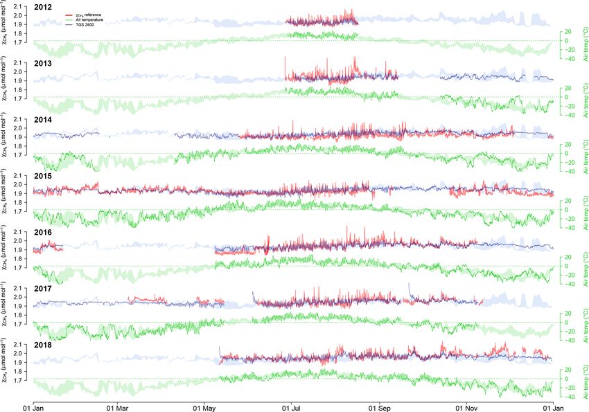
2682                                                  W. Eugster et al.: Long-term reliability of a solid-state methane sensor

complex rural and urban environments along the Colorado
Front Range (Collier-Oxandale et al., 2018), in an oil and gas
production region (Greeley, Colorado; Casey et al., 2019),
and in urban south Los Angeles (Shamasunder et al., 2018).
An application on an unmanned aerial vehicle, however, did
not successfully detect CH4 hotspots (Falabella et al., 2018).
These are all pioneering studies but are mostly restricted to a
few days to months of measurements. Thus, our study is the
first long-term comparison of high-precision measurements
to those from CH4 sensitive, low-cost sensors under chal-
lenging climatic conditions.
   Typically, new sensors are first calibrated under controlled
conditions in a laboratory environment. Extensive calibra-
tion tests with a similar low-cost sensor (Figaro TGS2611-
E00) from the same manufacturer as our TGS 2600 have               Figure 1. Two TGS 2600 trace gas sensors and the LinPicco A05
been carried out by van den Bossche et al. (2017). De-             temperature and relative humidity sensor (a) inside the weather pro-
spite the care taken in their calibration effort, the residual     tection and (b) the mounting position of the TGS weather protection
CH4 mole fraction after calibration was still on the order         and reference CH4 gas inlets at the Toolik wet sedge eddy covari-
of ±1.7 µmol mol−1 , which is acceptable for chamber flux          ance flux site.
measurements, for example, over water (as done by, e.g.,
Duc et al., 2019) but not sufficient to measure ambient at-
mospheric mole fractions, which are of the same order of           until 15 June 2016, with the continuation as a meteorolog-
magnitude as the calibration uncertainty. The issue of impor-      ical station until present. The site is a wetland that is a lo-
tant differences between laboratory assessments of low-cost        cal source of CH4 with a flux rate that is roughly 1 order
sensors and their real-world performance is well known and         of magnitude stronger than adjacent Toolik Lake, where the
typically relates to different data correction and calibration     Eugster and Kling (2012) study was performed. The site is
approaches in real-world rather than laboratory applications       a wet graminoid tundra dominated by sedge species, namely
(Lewis et al., 2018). Hence we decided to use outdoor mea-         cotton grass (Eriophorum angustifolium) and Carex aquatilis
surements obtained over a wide range of temperatures and           (Walker and Everett, 1991).
relative humidity – the major cross-sensitivities experienced
by such sensors – and derive a calibration function via pa-        2.2   Instrumentation and measurements
rameter extraction using this dataset. Our goals were thus to
(1) establish a statistical calibration function from field mea-   Two Figaro TGS 2600 sensors (Figaro, 2005a, b) that were
sured conditions that can also be used in different contexts to    already deployed over Toolik Lake (TOL) during the ice-free
linearize the TGS 2600 sensor signal (which then can still be      season in 2011 (Eugster and Kling, 2012) were installed at
fine-tuned with a two-point calibration in a specific applica-     the TWE site in late June 2012 (Fig. 1). Sensor 1 is the pri-
tion); (2) assess the reliability of the TGS 2600 low-cost sen-    mary sensor used in this study, whereas sensor 2 was only
sor under winter and summer conditions in the Arctic over          used as a replicate to simplify assessing potential problems
7 years of continuous deployment; and (3) explore poten-           with sensor 1. Because no such problems occurred, we will
tial improvements for sensor data processing, which includes       focus only on the results obtained with sensor 1 except in
(3a) wind effects that are neglected in laboratory environ-        Sect. 3.2, where we used both sensors to assess their perfor-
ments and (3b) artificial neural networks (ANNs) to find out       mance at weekly time resolution. The TGS 2600 is a high-
whether results can be improved over standard statistical re-      sensitivity solid-state sensor for the detection of air con-
gression methods for calibration of the sensor.                    taminants (Figaro, 2005a). It is sensitive to methane at low
                                                                   mole fractions but also to hydrogen, carbon monoxide, isobu-
                                                                   tane, and ethanol. It is the only low-cost solid-state sensor
2     Material and methods                                         that we are aware of for which the manufacturer indicates a
                                                                   sensitivity to methane even under ambient (≈ 2 µmol mol−1 )
2.1    Study site                                                  methane mole fractions, whereas most other sensors are only
                                                                   sensitive at mole fractions that exceed ambient levels by at
Field measurements were carried out at the Toolik wet sedge        least 1 or 2 orders of magnitude. This high sensitivity to low-
site (TWE; 68◦ 370 27.6200 N, 149◦ 360 08.1000 W; 728.14 m ele-    methane mole fractions comes at the expense that no specific
vation, WGS 84 datum) where seasonal eddy covariance flux          molecular filter prevents the other components from reach-
measurements were carried out during the summer seasons            ing the sensor surface. Thus, our considerations made here
of 2010–2015 and partially during winters starting in 2014         assume that deployment is made in an area like the Arctic,

Atmos. Meas. Tech., 13, 2681–2695, 2020                                              https://doi.org/10.5194/amt-13-2681-2020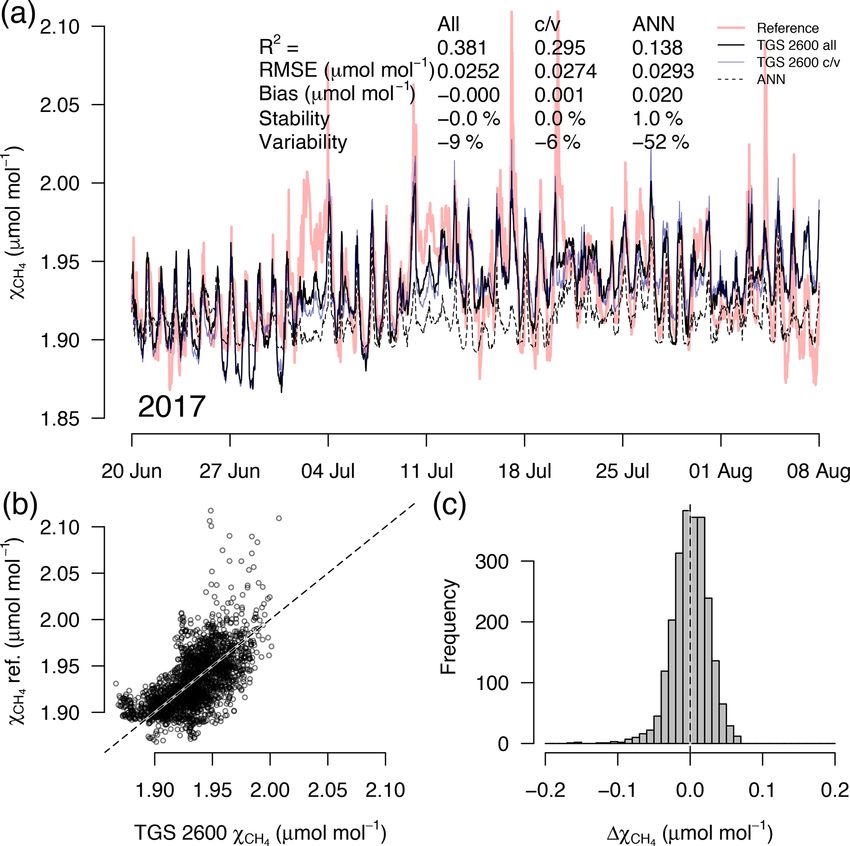
W. Eugster et al.: Long-term reliability of a solid-state methane sensor                                                   2683

where levels of carbon monoxide, isobutane, ethanol, and          in the early summer season, when field personnel arrived at
hydrogen are rather constant and do not vary as strongly as       TFS (late May).
methane so that the sensor signal can be interpreted as a first      Because the TGS 2600 sensors only show a weak response
approximation of a methane mole fraction signal. For addi-        to CH4 but are highly sensitive to temperature and humid-
tional details on the TGS 2600 sensor the reader is referred      ity, a LinPicco A05 Basic sensor (IST Innovative Sensor
to Eugster and Kling (2012).                                      Technology, Wattwil, Switzerland) was added next to the
   The TWE site receives line power from the Toolik Field         TGS 2600 (see Fig. 1). The A05 is a capacitive humidity
Station (TFS) power generator. During the snow- and ice-          module that also has a Pt1000 platinum 1 k thermistor on
free summer season (typically late June to mid-August) mea-       board to measure ambient temperature. The relative humid-
surements are almost interruption-free, but during the cold       ity output by the A05 is a linearized voltage in the range of
season (typically September to late May) longer power in-         0–5 V, and the Pt1000 thermistor was measured in three-wire
terruptions limit the winter data coverage. Nevertheless, this    half-bridge mode using an excitation voltage of 4.897 V.
is the first study that provides low-cost sensor methane mole
fraction measurements over a temperature range from Arctic        2.3   Calculations
winter temperatures of −41 ◦ C to a relatively balmy 27 ◦ C
during short periods of the Arctic summer. Reference CH4          Before analyses the data were processed in the following
dry mole fractions were measured by a Fast Methane Ana-           way: (1) outliers were removed (2) relative humidities greater
lyzer (FMA, Los Gatos Research, Inc., San Jose, CA, USA;          than 105 % (accuracy of capacitive humidity sensors) were
years 2012–2016), which was replaced by a Fast Greenhouse         deleted, and (3) reference CH4 mole fractions obtained from
Gas Analyzer (FGGA, Los Gatos Research, Inc., San Jose,           the FGGA (since 2016) were filtered based on hard bound-
CA, USA; since 2016) for combined CH4 , CO2 , and H2 O            aries of housekeeping variables available for quality control.
dry mole fraction measurements. Until 18 June 2016 the CH4        For the latter we used the following hard boundaries for fil-
mole fractions were calculated as 1 min averages from the         tering: (a) sample cell pressure had to be in the range of
raw eddy covariance flux data files. We report all gas mole       130–143 Torr and (b) the instrument-specific ringdown time
fractions in micromoles per mole or nanomoles per mole.           of the laser for CH4 measurements had to be in the range of
The FMA and FGGA sampling rate was set to 20 Hz, and              13–17 ms. The accepted reference CH4 mole fractions were
the flow rate of sample air was ca. 20 L min−1 . After the ter-   thus all measured in the narrow range of cell pressures be-
mination of eddy covariance flux measurements, the FGGA           tween 139.7 and 140.3 Torr and laser ringdown times be-
measurements were continued with the instrument’s inter-          tween 14.02 and 14.94 ms, which indicates best performance
nal pump (flow rate ca. 0.65 L min−1 ) with 1 Hz raw data         of the analyzer. Before 2016 (FMA instrument) these house-
sampling. In addition to digital recording, the CH4 signal        keeping variables were not recorded.
was converted to an analog voltage that was recorded on a            The basic principle of operation of the TGS 2600 sensor
CR23X data logger (Campbell Scientific Inc., CSI, Logan,          was described in detail by Eugster and Kling (2012). The
UT, USA). The same data logger also recorded air temper-          methane sensing mechanisms of different active materials
ature, relative humidity (HMP45AC, CSI), wind speed, and          used in solid-state sensors were described by Aghagoli and
wind direction (034B Windset, MetOne, Grants Pass, OR,            Ardyanian (2018). The TGS 2600 uses an SnO2 microcrys-
USA) as well as ancillary meteorological and soil variables       tal surface (Figaro, 2005b). Whereas the manufacturer de-
not used in this study. The factory-calibrated HMP45AC sen-       fines the sensor signal as Rs /R0 , the ratio of the electrical
sor head was exchanged for a newly calibrated one ca. ev-         resistance Rs of the heated sensor material surface normal-
ery 3 years to minimize long-term drift effects in temperature    ized over its resistance R0 in the air under absence of CH4 ,
and relative humidity measurements (James Laundre, per-           Hu et al. (2016) define the sensor signal as the ratio between
sonal communication, 2020). Sensors were measured every           Rs and Rg , the resistance of the surface in the pure gas of
5 s, and 1 min averages were stored on the logger. These data     interest (here CH4 ). In all cases, considerations of techni-
were then screened for outliers and instrumental errors and       cal sensor information are made for high mole fractions of
failures, and 30 min averages were calculated for the present     CH4 (e.g., 200 µmol mol−1 ) for an SnO2 surface according
analysis.                                                         to Hu et al. (2016), not for ambient mole fractions in the typ-
   Both FMA and the later FGGA analyzers were used for            ical range of 1.7–4 µmol mol−1 (or less). Hence, some adap-
eddy covariance applications, and thus the instruments were       tations are always necessary because present-day sensors are
not calibrated as frequently as is done in applications for the   not yet designed for such low mole fractions. In order to sim-
Global Atmosphere Watch network (WMO, 2001). Both sen-            plify calculations compared to what we presented in Eugster
sors were more accurate than the available calibration CH4        and Kling (2012) – which closely followed the technical in-
gases at TFS. In 2015 it was possible for the first time to use   formation provided by the manufacturer (Figaro, 2005a, b) –
an NOAA (National Oceanographic and Atmospheric Ad-               we define the sensor signal as Sc = Rs /R0 but with R0 arbi-
ministration, Boulder, CO, USA) reference gas cylinder (no.       trarily set to the resistance observed when the sensor delivers
CB09837) to fine-tune the FGGA. This was typically done           V0 = 0.8 V output at Vc = 5.0 V supply voltage. The high-

https://doi.org/10.5194/amt-13-2681-2020                                           Atmos. Meas. Tech., 13, 2681–2695, 2020
2684                                                 W. Eugster et al.: Long-term reliability of a solid-state methane sensor

est voltages measured at TWE were 0.7501 and 0.7683 V
from sensors 1 and 2, respectively (which theoretically cor-
responds to the lowest CH4 mole fractions). With these as-
sumptions the sensor signal Sc can easily be approximated as
a function of the inverse of the measured TGS signal voltage
Vs ,
       Rs              1
Sc =      ≈ 0.952381 ·    − 0.1904762 .                    (1)
       R0              Vs
The full derivation is
     Vc ·RL              Vc ·RL −Vs ·RL                           Figure 2. Difference between TGS 2600 and reference CH4 mea-
Rs    V      − RL              Vs
   = V ·Rs        =                       =                       surements (30 min averages) as a function of air temperature when
R0    c    L             Vc ·RL −Vs ·RL                           using the Eugster and Kling (2012) conversion. Agreement was
      V0 − RL                  V0
                                                                  good when ambient temperature was above freezing. The horizontal
        V0 (Vc − Vs ) RL   V0 (Vc − Vs )                          color bar shows the ±0.1 µmol mol−1 range around a perfect agree-
      =                  =               =
        Vs (Vc − V0 ) RL   V (V − V0 )                            ment. The green band shows the interquartile range of bin-averaged
                         s c
           V0     Vc           1 Vc · V0     V0                   differences (TGS 2600 sensor 1), and dashed lines show the extent
      =                −1 =      ·         −     .                of the 95 % confidence intervals. Gray bars at the bottom show the
        Vc − V0 Vs            Vs Vc − V0 Vc − V0
                                                                  number of 30 min averages in each bin. The scale bar (1000 h) on
Here RL is the load resistor over which Vs is measured (see       the right specifies their size.
Figaro, 2005a, or Eugster and Kling, 2012, for more details)
but which can be eliminated in this algebraic simplification.
   To compute absolute humidity, we used the Magnus equa-         no detailed information on p values is given when statistical
tion to estimate saturation vapor pressure esat (in hPa) at am-   significance of trends or drift is mentioned in the following.
bient temperature Ta (in ◦ C),                                       For assessing the quality of the proposed calculation of
                                                                  CH4 mole fractions from TGS 2600 sensors we inspected
esat = 6.107 × 10a·Ta /(b+Ta ) ,                                  weekly aggregated data using four key indicators:
                                                                     Bias. This is the mean of the difference of each 30 min
with coefficients a = 7.5 and b = 235.0 for Ta ≥ 0 ◦ C and        averaged pair of CH4 mole fractions in micromoles per mole,
a = 9.5 and b = 265.5 for Ta < 0 ◦ C.                             CH4,TGS – CH4,ref .
  Actual vapor pressure e (hPa) was then determined as               Stability. This is the bias expressed as a percent devi-
                                                                  ation from the reference CH4 mole fraction, (CH4,TGS −
              RH
e = esat ·         ,                                              CH4,ref )/CH4,ref · 100 %.
             100 %                                                   Variability. This is the mean relative deviation of the 95 %
with relative humidity RH in percent and converted to abso-       confidence interval (CI) observed with the TGS 2600 sensor
lute humidity ρv (kg m−3 ) with                                   from the corresponding 95 % CI of the CH4 reference mea-
                                                                  surements (in percent), (CI95 %,TGS /CI95 %,ref − 1) · 100 %.
            e        p    100                e                       Correlation of median diel cycles. Pearson’s product-
ρv =              ·     ·     ≈ 0.217 ·             ,
       Ta + 273.15 p − e Rv             Ta + 273.15               moment correlation coefficient between hourly aggregated
                                                                  median diel cycles of CH4 measured by the TGS 2600 and
with p being atmospheric pressure (hPa) and Rv the gas con-       reference instruments.
stant for water vapor (461.53 J kg−1 K−1 ).                          In addition to conventional linear model fits (least
                                                                  square method) we used an ANN approach. This was
2.4    Statistical analyses
                                                                  performed in Python 3.7.1 using MLPRegressor from
Statistical analyses were performed with R version 3.5.2 (R       sklearn.neural_network version 0.20.2 (Pedregosa et al.,
Core Team, 2018). Trend analyses were performed for both          2011). We used a network with four hidden layers of sizes
trend in CH4 mole fraction and drift of TGS 2600 measure-         500, 100, 50, and 5, respectively, and an adaptive learning
ments using the Mann–Kendall trend test implemented in the        rate. Learning was done with the data obtained during the
rkt package that is based on Marchetto et al. (2013). The an-     calibration period 2014–2016, whereas the remaining years
nual linear trend (or drift) was calculated using the robust      2012–2013 and 2017–2018 were used for validation.
Theil–Sen estimator (Akritas et al., 1995) using weekly me-
dian values, and the significance of the trend (or drift) was
assessed using Kendall’s τ parameter. All trend and drift es-
timates were significant at p < 0.05. The highest two-sided
p value of the presented results was p = 0.000054, and thus

Atmos. Meas. Tech., 13, 2681–2695, 2020                                             https://doi.org/10.5194/amt-13-2681-2020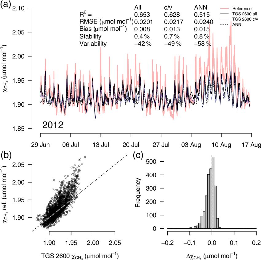
W. Eugster et al.: Long-term reliability of a solid-state methane sensor                                                         2685

                                                                       tive humidity but to either actual vapor pressure (in hPa) or
                                                                       absolute humidity (in kg m−3 ). In all tested models absolute
                                                                       humidity performed marginally better than vapor pressure or
                                                                       mixing ratio (measured by R 2 ; not shown); hence we sug-
                                                                       gest the following model and parameterization to estimate
                                                                       CH4 mole fractions in micromoles per mole from TGS 2600
                                                                       signal voltage measurements:

                                                                       CH4 =1.425 + 0.12 Sc + 0.375/Sc − 0.0065 Ta +
                                                                               + 53.3 ρv + 0.0022 Sc · Ta − 0.0017 Ta /Sc +
                                                                               + 4.9 Sc · ρv − 67.4 ρv /Sc − 0.39 Sc · Ta · ρv
                                                                               + 1.15 Ta · ρv /Sc ,                               (2)

                                                                       with Sc being the dimensionless sensor signal (see Eq. 1),
                                                                       Ta the ambient air temperature in ◦ C, and ρv the absolute hu-
                                                                       midity in kilograms per cubic meter. The parameter estimates
                                                                       were derived from the entire 2012–2018 dataset for TGS sen-
                                                                       sor 1 (Table 1, “entire period”). For other sensors the result
                                                                       from Eq. (2) can be considered as a linearized signal that can
                                                                       be fine-tuned with a sensor-specific two-point calibration as
Figure 3. Difference between TGS 2600 and reference CH4 mea-           suggested in Sect. 3.4 of Eugster and Kling (2012).
surements (30 min averages) as a function of (a) relative humidity        The linear model in Eq. (2) was derived from a suite
(in %) and (b) absolute humidity (in kg m−3 ). The horizontal color    of candidate models including interactions among predic-
bar shows the ±0.1 µmol mol−1 range around a perfect agreement.        tors and quadratic terms of each variable, and then step-
The green band shows the interquartile range of bin-averaged differ-
                                                                       wise elimination using the stepAIC function in the MASS
ences (TGS 2600 sensor 1), and dashed lines show the extent of the
95 % confidence intervals. Gray bars at the bottom show the number
                                                                       package of R was employed to find the model with the low-
of 30 min averages in each bin. The scale bar (1000 h) on the right    est AIC (Akaike’s information criterion). Unless explicitly
specifies their size.                                                  mentioned, we analyzed CH4 mole fractions computed with
                                                                       Eq. (2) using the parameters obtained from all data measured
                                                                       by TGS 2600 sensor 1. Only in the direct comparison with
                                                                       the ANN (Sect. 3.1) did we determine an additional param-
3   Results and discussion
                                                                       eter set using the same calibration period as the ANN used
                                                                       (Sect. 2.4), making a direct comparison of performance in
CH4 mole fractions estimated from TGS 2600 measurements                validation possible.
during the cold seasons differed strongly from the reference              If ambient temperature influences the signal of the
measurements when the Eugster and Kling (2012) approach                TGS 2600 in such a way as expected from the technical doc-
was used (not shown); that approach translated the informa-            umentation (Figaro, 2005a, b), then wind speed could be a
tion from the technical specifications of the TGS 2600 sen-            third factor influencing the conversion from TGS 2600 sen-
sor (Figaro, 2005a, b) to outdoor applications. The agree-             sor voltages to CH4 mole fractions. To investigate this addi-
ment with the CH4 reference measurements was within                    tional factor, we produced a heat loss model, assuming that
±0.1 µmol mol−1 with temperatures above freezing (Fig. 2)              the sensor correction is related to the cooling of the heated
but not so during cold conditions (Ta < 0 ◦ C). The differ-            surface of the solid-state sensor, which has a nominal surface
ences between TGS estimates and CH4 reference measure-                 temperature Ts of 400 ◦ C (Falabella et al., 2018). This is the
ments were largest with the Eugster and Kling (2012) ap-               typical operation temperature of SnO2 –Ni2 O3 sensors (Hu
proach when relative humidity was between 50 % and 90 %                et al., 2016). Our candidate model for heat loss (HL in W)
(Fig. 3a). When converting relative humidity to absolute hu-           was
midity, the results became satisfactory for absolute humidity
values greater than 0.004 kg m−3 (Fig. 3b). Using absolute             HL ∼ ξ · u2 · (Ts − Ta ) · (ρd · Cd + ρv · Cv ) ,          (3)
humidity in place of relative humidity for the correction of
the TGS 2600 was already attempted by Collier-Oxandale                 with u being mean horizontal wind speed (m s−1 ), Ts and
et al. (2018); this contrasts with the manufacturer’s sug-             Ta the sensor surface and ambient air temperature (K), re-
gestion (Figaro, 2005a). Because absolute humidity above               spectively, ρd the density of dry air (kg m−3 ), ρv the abso-
0.004 kg m−3 is only possible at temperatures above 0 ◦ C it           lute humidity (kg m−3 ), and Cd and Cv the heat capacity of
appears quite obvious that temperature and humidity correc-            dry air and water vapor, respectively (J kg−1 K−1 ). The scal-
tions of solid-state sensors most likely do not relate to rela-        ing coefficient ξ is a best-fit model parameter (units: s m).

https://doi.org/10.5194/amt-13-2681-2020                                                  Atmos. Meas. Tech., 13, 2681–2695, 2020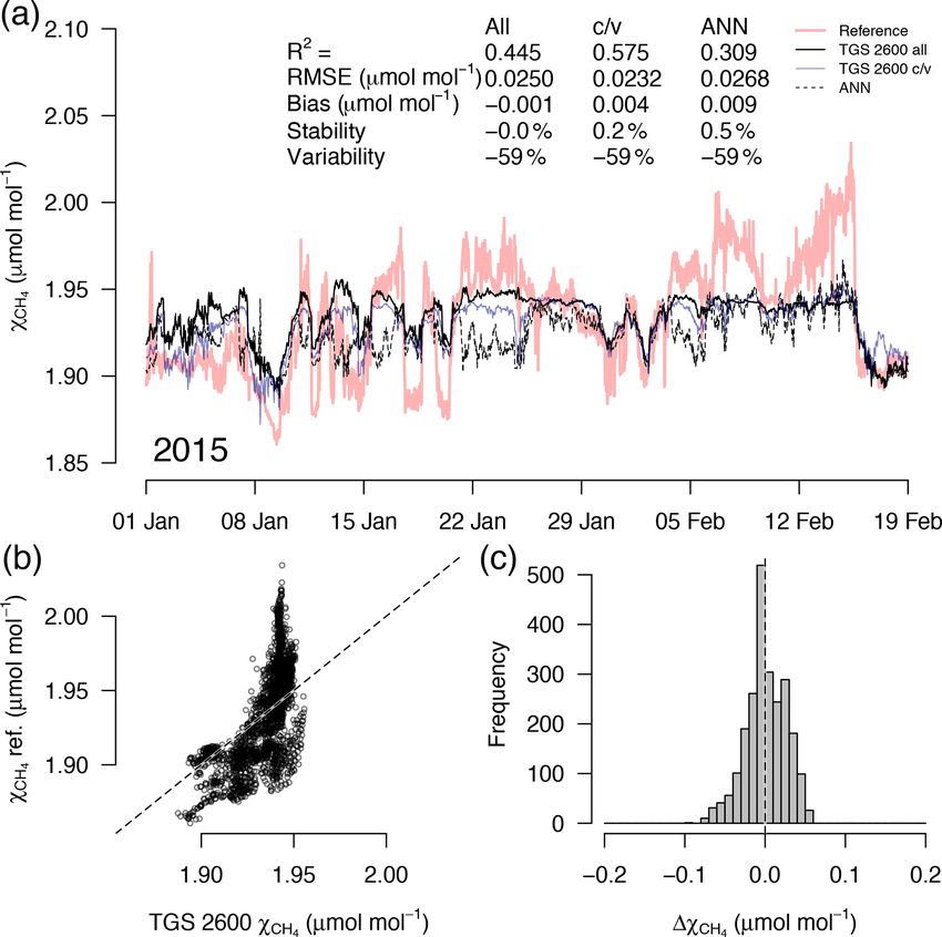
2686 W. Eugster et al.: Long-term reliability of a solid-state methane sensor
Table 1. Goodness of fit of TGS 2600 (sensor 1)-derived CH4 mole fractions (30 min averages) obtained from a linear model using air
temperature and absolute humidity (Eq. 2), a heat loss model (Eq. 3), and an artificial neural network (ANN). For the goodness of fit the
coefficient of determination (R 2 ) and the root mean square error (RMSE) of the residuals are reported for the overall model and separately
for warm and cold conditions. The parametrization of the linear model given in Eq. (2) used the entire 2012–2018 period. For a more
rigorous model test, all three approaches were calibrated with the data measured in years 2014–2016, and the remaining data (2012–2013
and 2017–2018) were used for validation.
Linear model Heat loss model Artificial neural network
Entire period Calibration Validation Calibration Validation Calibration Validation
Overall
R2 0.424 0.447 0.207 0.166 0.284 0.311 0.282
RMSE (µmol mol−1 ) 0.030 0.026 0.041 0.032 0.046 0.030 0.043
Warm conditions (Ta ≥ 0 ◦ C)
R2 0.476 0.518 0.288 0.180 0.181 0.278 0.265
RMSE (µmol mol−1 ) 0.027 0.026 0.032 0.034 0.039 0.032 0.036
Cold conditions (Ta < 0 ◦ C)
R2 0.322 0.345 0.034 0.157 0.055 0.314 0.092
RMSE (µmol mol−1 ) 0.033 0.027 0.052 0.031 0.055 0.028 0.053
The assumption made here was that the wind speed governs vs. 0.00 µmol mol−1 and 0.0 %, respectively). In winter the
the eddy diffusivity of heat transported along the temperature timing of most events is correctly captured (Fig. 7) with an
gradient between the sensor surface and ambient air, and the R 2 of 0.445, but the dynamics are not satisfactorily captured
moisture correction is only associated with the fact that water by the TGS sensor, indicated by a 59 % underestimation of
vapor has a higher heat capacity (1859 J kg−1 K−1 ) than dry the 95 % CI during this midwinter period. The transition from
air (1005.5 J kg−1 K−1 ), and hence the heat capacity of moist warm to cold season (Fig. 8) shows a mixture of days when
air increases accordingly with ρv . the regular diel cycle, which is typical for the warm sea-
son, is still adequately captured, but the dynamics of periods
3.1 Performance of the TGS 2600 sensor at 30 min with an air temperature below 0 ◦ C (see Fig. 4), when CH4
resolution mole fractions tend to be highest as in winter (Fig. 7), are
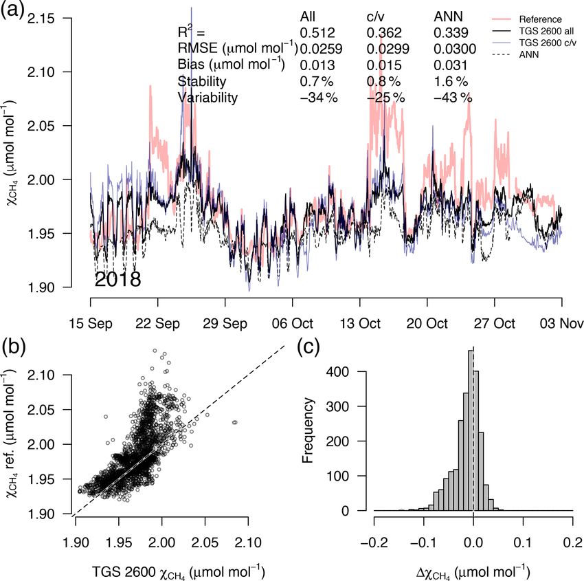
not adequately captured. Still, with an R 2 of 0.512 (Fig. 8)
Using Eq. (2) yields satisfying agreement with 30 min aver- more than 50 % of the variance observed in the 30 min av-
aged data under both typical low-Arctic summer and winter eraged CH4 reference measurements is captured by the low-
conditions (Fig. 4) with an overall R 2 of 0.424 (Table 1). cost TGS 2600 sensor.
When testing the linear model approach (Eq. 2) more rigor- Because of the absence of local sources of carbon monox-
ously by splitting the available data into a calibration period ide and other air pollutants to which the TGS 2600 sensor is
(years 2014–2016) and a validation period (years 2012–2013 also sensitive (besides CH4 ), we investigated a special case
and 2017–2018), some limitations can be seen, in particu- when smoke and haze from wildfires south of the Books
lar under cold conditions, where none of the approaches per- Range polluted the air in the TFS area on 26 June 2015
formed very well in the validation period. The ANN had a and compared the performance of both TGS sensors dur-
more balanced performance between the calibration and vali- ing that day with conditions 3 d before that event and on
dation periods, although it performed slightly less well under the same date in the following 3 years. The net effect
warm conditions (Ta ≥ 0 ◦ C). of increased air pollutants was an apparent small decrease
A detailed inspection of four representative 7-week time in the CH4 mole fractions calculated via Eq. (2) by ap-
periods at full 30 min resolution is shown in Figs. 5–8. Typi- proximately −0.03 µmol mol−1 . At the same time the vari-
cal summer conditions at the beginning of this study (Fig. 5) ability of the residuals increased from typically ±0.014 to
and towards the end of the analyzed period (Fig. 6) indicate ±0.027 µmol mol−1 (24 h averages). Thus, the influence of
that the short-term agreement (R 2 = 0.653; Fig. 5) was bet- the wildfire smoke was of the same order of magnitude as
ter when the TGS sensor was still relatively new than when the difference between TGS-derived CH4 mole fractions and
it was 7 years old (R 2 = 0.381; Fig. 6), but the variability the reference instrument on most other days of the year (see
decreased (improved) from −42 % to −9 % with no relevant Figs. 5–8).
difference in bias and stability (0.01 µmol mol−1 and 0.4 %
Atmos. Meas. Tech., 13, 2681–2695, 2020 https://doi.org/10.5194/amt-13-2681-2020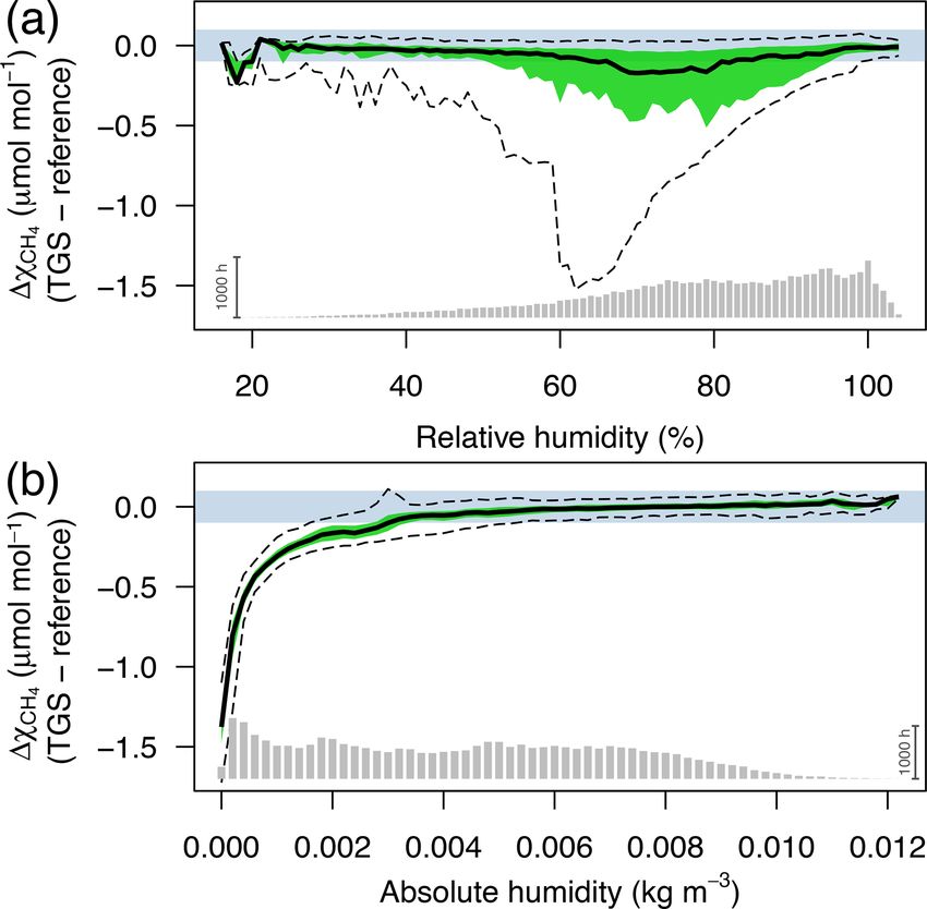
W. Eugster et al.: Long-term reliability of a solid-state methane sensor                                                              2687

Figure 4. Overview over annual courses of 30 min averaged air temperature (green) and CH4 mole fractions (blue and red). Pale color bands
show the daily interquartile range (50 % of values between the first and third quartiles) of measurements from all years. Solid lines show
actual measurements. Red lines are the reference CH4 measurements, and blue lines show the CH4 mole fraction derived from TGS 2600
measurements (sensor 1). Actual measurements show 30 min mean values.

3.2   Performance of weekly aggregated data                            be measurable after 10–13 years of continuous operation, in-
                                                                       dicating the end of life of a TGS 2600.
The TGS 2600 is not expected to provide short-term accu-                  Figure 10 shows the weekly median bias, variability, and
racy comparable to high-quality instrumentation (see also              the correlation between the weekly aggregated median diel
Lewis et al., 2018). However, Eugster and Kling (2012) ar-             cycle of CH4 at hourly resolution between the TGS 1 mea-
gued that such measurements may still provide additional in-           surements and the reference. Despite the trend of the sensor
sights as compared to the passive samplers described by God-           signal shown in Fig. 9a and b, both the bias and variabil-
bout et al. (2006a, b) by integrating over longer time frames.         ity primarily show a seasonal pattern with a slightly nega-
Thus, here we inspected the performance of weekly aggre-               tive bias (around −0.02 µmol mol−1 ) during peak growing
gated estimates derived from the TGS 2600 in order to in-              season and a corresponding positive deviation in midwinter
spect drift of the two sensors and their performance over the          when temperatures can be well below −30 ◦ C (Fig. 10a). The
7-year deployment period. Note that in Eq. (2) we did not              variability (Fig. 10b) shows the inverse pattern of the bias. If
include a drift correction. Figure 9 shows weekly medians              bias is expressed as the relative bias (i.e., stability), the stabil-
of sensor signals, the agreement with the reference signal,            ity vs. variability plot (Fig. 11) shows points lying uniformly
and the difference between the CH4 mole fractions obtained             around the line of a −1 : 1 relationship (R 2 = 0.67). This in-
from both TGS 2600 sensors mounted at the same position                dicates that both variability and stability can be improved at
(Fig. 1). The two TGS 2600 sensors (1 and 2) showed a trend            the same time because there is no tradeoff visible in Fig. 11.
in their signals of −18.8 and −15.5 mV yr−1 , respectively
(Fig. 9a). Thus, with typical signals on the order of 200–
700 mV (Fig. 9a) the lowest (winter) readings may no longer

https://doi.org/10.5194/amt-13-2681-2020                                                  Atmos. Meas. Tech., 13, 2681–2695, 2020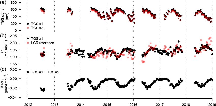
2688                                                     W. Eugster et al.: Long-term reliability of a solid-state methane sensor

Figure 5. (a) Time series of TGS 1-derived CH4 during a 7-week snow- and ice-free period in the first year of the long-term deployment
(2012), (b) correlation with reference mole fraction, and (c) residuals (TGS 2600 all minus the reference) of 30 min averaged measurements.
Thin solid lines in (a) show the result when all data are used with Eq. (2), reference mole fraction is shown with a red bold line, c/v shows
an alternative fit from splitting the available data into a calibration and a validation part, and the dashed line shows the performance of an
artificial neural network (ANN) fit. This example belongs to the validation period of the TGS 2600 c/v and ANN fits.

3.3    Linear trend and drift estimates                                  it remains a challenge to deduce the true trend in CH4 mole
                                                                         fractions over longer time periods using such a low-cost sen-
All linear trend estimates were statistically significant (see           sor because of drifting signals. Thus, we inspected the drift
Sect. 2.4). However, our measurements started with warm-                 of the TGS 2600-derived mole fraction with respect to the
season measurements only (2012–2014) that were succes-                   (true) CH4 trend observed with the high-quality reference
sively expanded to include cold-season measurements. Thus,               instrument. These drifts appear to be smaller than the true
all interpretation of the trends and drifts presented here               trend but are still considerable: the bias of TGS-derived CH4
should be considered with caution given the long gaps in data            mole fractions drifted by 4–6 nmol mol−1 yr−1 (40 %–60 %
due to the technical challenges of operating such equipment              of actual trend), and variability drifted by −0.24 % yr−1 .
under adverse winter conditions. The CH4 mole fraction                   They provide encouraging results suggesting that with occa-
trend observed with the high-quality reference measurements              sional (infrequent) calibration with a high-quality standard,
was 10.1 nmol mol−1 yr−1 . This is 2.5 times the trend ob-               e.g., using a traveling standard operating during a few good
served from 2005 to 2011 by NOAA (28.6 ± 0.9 nmol mol−1                  days with adequate coverage of the near-surface diel cycle
or 4.09 nmol mol−1 yr−1 ; Table 2.1 in Hartmann et al., 2014)            of CH4 , TGS 2600 measurements might be suitable for the
but of the same order of magnitude reported by Nisbet et al.             monitoring of CH4 mole fractions in other areas as well. As
(2014) for 2013 (last year covered by that study) for lati-              shown in Fig. 10c the correlation of median diel cycles be-
tudes north of the Tropic of Cancer. Thus, this trend may be             tween TGS estimates and CH4 reference measurements is
real, and hence all trends seen in low-cost sensor signals are           one of the weak points in the current performance of the
not necessarily solely an artifact of such sensors. However,             TGS 2600 sensors. Furthermore, we observed a significant

Atmos. Meas. Tech., 13, 2681–2695, 2020                                                     https://doi.org/10.5194/amt-13-2681-2020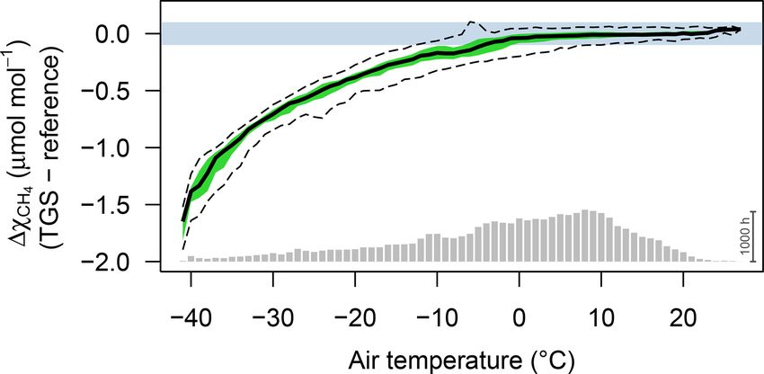
W. Eugster et al.: Long-term reliability of a solid-state methane sensor                                                       2689

Figure 6. As in Fig. 5 but with measurements from a 7-week snow- and ice-free period in 2017 at a sensor age of 7 years. This example
belongs to the validation period of the TGS 2600 c/v and ANN fits.

negative trend of the correlation coefficient of −0.051 yr−1         ter, with temperatures below freezing, the ANN performed
(Fig. 10c). However, the key finding is that the typical diel        clearly better in the validation than the linear approach, but
cycle during the warm season (air temperature > 0 ◦ C) disap-        both approaches remained unsatisfactory (R 2 < 0.1) despite
pears during winter conditions (Figs. 4, 7), and thus separate       the fact that both approaches were similar in the calibration
transfer functions for warm and cold temperatures might be a         period (R 2 ≈ 0.3, Table 1).
solution for future studies (Table 1). Our Eq. (2) is thus inten-       During the warm period we found cases where the ANN
tionally derived from the entire dataset to provide a starting       was much better in capturing a specific daily feature, as for
point for more elaborate fine-tuning in projects where this is       example on 11 July 2012 (Fig. 5a), when the daily mini-
desired.                                                             mum was nicely captured by the ANN, but the linear model
                                                                     was much too low. Contrastingly, in 2017 (Fig. 6a) periods
3.4   Potential of using artificial neural networks                  could be found when the daily dynamics were correctly cap-
                                                                     tured by the ANN but at too low of mixing ratios (e.g., 10–
Casey et al. (2019) found that artificial neural networks            18 July 2017; Fig. 6a). It should be noted that at this lati-
(ANNs) outperformed linear models in mitigating curvature            tude the sun does not set between 24 May and 20 July; thus
and linear trends in trace gas measurements when used with           nocturnal conditions are clearly different from conditions at
the same set of input variables during a 3-month compari-            lower latitudes such as the ones investigated by Casey et al.
son period. To inspect the potential of ANNs at our Arctic           (2019). Similarly, the transition from warm to cold season
long-term dataset, we added the ANN results to Figs. 5–8.            (Fig. 8) was challenging with both the linear model and ANN
In summer (Figs. 5, 6) we did not find a substantial differ-         approach. We have only used two variables, Ta and humidity,
ence between an ANN and the linear approach of Eq. (2) in            that according to manufacturer specifications (Figaro, 2005a,
terms of root mean square error (RMSE) or R 2 between pre-           b) influence the TGS 2600 sensor signal. In reality, the same
dicted and measured CH4 mole fractions (Table 1). In win-

https://doi.org/10.5194/amt-13-2681-2020                                               Atmos. Meas. Tech., 13, 2681–2695, 2020
2690 W. Eugster et al.: Long-term reliability of a solid-state methane sensor
Figure 7. As in Fig. 5 but with measurements from a 7-week period in midwinter with temperatures plunging down to −40 ◦ C. High CH4
mole fractions coincide with the coldest temperatures (see Fig. 4). This example belongs to the validation period of the TGS 2600 c/v and
ANN fits.
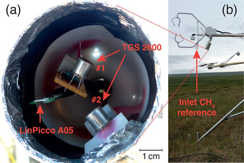
two variables also influence the CH4 production in water- age is poor (gray bars at bottom of Fig. 12a) as temperatures
logged ecosystems and thus contribute to the true CH4 signal below −30 ◦ C were not frequently covered due to technical
in addition to the cross-sensitivity, which we try to correct problems with the measurement station and summer temper-
with Eq. (2). atures above 20 ◦ C are still rather rare at this low-Arctic lat-
An ANN that can separate the effect of ambient variations itude (Hobbie and Kling, 2014). A slightly different picture
of CH4 mole fractions from the artifact of cross-sensitivity emerges for low absolute humidity: 56 % of measurements
of the TGS 2600 to Ta and humidity may however outper- are at lower humidities than the saturation humidity at 0 ◦ C
form a linear model approach in future studies if more po- (0.0049 kg m−3 ); thus the rather homogenous variances at
tentially important driving variables are included than only low humidity (Fig. 12b) indicate that humidity is not of con-
those specified by the manufacturer (Figaro, 2005a, b). cern at low temperatures, and future attempts for improve-
ments should rather focus on humidity above 0.01 kg m−3
3.5 Suggestions for future work and temperatures above 20 ◦ C that are not normally found in
the Arctic.
The interquartile ranges and 95 % confidence intervals of Based on physical considerations one might expect that
each air temperature (Fig. 12a) or absolute humidity bin specific humidity or water vapor mixing ratio instead of abso-
(Fig. 12b) are very similar over a wide range of tempera- lute humidity could lead to further improvements because ab-
tures and humidity levels but tend to become more variable in solute humidity still depends on temperature. However, our
bins with few data (i.e., lowest and highest temperatures and tests have not indicated a relevant gain of information or ac-
highest absolute humidities in Fig. 12). Deviations are gen- curacy of prediction, but future work should also try to find
erally constrained within ±0.1 µmol mol−1 or better but with a better physical correction model than the purely empirical
higher variability at both temperature ends, where data cover- one used here based on manufacturer information.
Atmos. Meas. Tech., 13, 2681–2695, 2020 https://doi.org/10.5194/amt-13-2681-2020W. Eugster et al.: Long-term reliability of a solid-state methane sensor 2691 Figure 8. As in Fig. 5 but with measurements from a 7-week period during the transition from fall to early winter. This example belongs to the validation period of the TGS 2600 c/v and ANN fits. Figure 9. (a) Weekly median sensor signals from both TGS 2600 sensors, (b) CH4 derived with Eq. (2) for TGS sensor 1 and measured by the Los Gatos Research reference instrument, and (c) absolute difference between the two TGS 2600 sensors. The signals from both sensors were converted to CH4 using Eq. (2) parameterized with data from TGS sensor 1. Symbol size is proportional to relative data coverage. https://doi.org/10.5194/amt-13-2681-2020 Atmos. Meas. Tech., 13, 2681–2695, 2020
2692                                                      W. Eugster et al.: Long-term reliability of a solid-state methane sensor

Figure 10. (a) Weekly median bias, (b) median variability, and (c) correlation between weekly median diel cycles of TGS 2600 sensor 1 and
the reference. Symbol size is proportional to relative data coverage.

Figure 11. Variability and stability (relative bias) of weekly median
TGS 2600 sensor 1-derived CH4 mole fractions are inversely related
and plotted along the −1 : 1 line. Symbol size is proportional to
relative data coverage.

                                                                        Figure 12. Residuals of 30 min averaged TGS 2600 vs. refer-
   Another approach was taken by van den Bossche et al.                 ence CH4 measurements as a function of (a) air temperature and
(2017), who performed an in-depth laboratory calibration                (b) absolute humidity. Colored areas show the interquartile range
of the very similar but less sensitive Figaro TGS 2611-E00              (50 % CI), bold lines show the median, and dashed lines show
sensor (the manufacturer only specifies a response above                the bin-averaged 95 % confidence interval. Bin size was 1 ◦ C and
300 µmol mol−1 CH4 ; Figaro, 2013) at different tempera-                0.0002 kg m−3 , respectively. Gray bars at the bottom show the num-
                                                                        ber of 30 min averages in each bin; the scale bar (1000 h) on the
tures and levels of relative humidity over a CH4 calibration
                                                                        right specifies their size.
range starting at ≈ 2 µmol mol−1 ambient mole fraction up
to 10 µmol mol−1 CH4 . Despite the effort, the residual mole
fractions remained large (range of ca. −1.5 µmol mol−1 to
+1.1 µmol mol−1 ) – too large for the application we present            et al. (2014) are convinced that “to be of use for advanced ap-
here. Our efforts to calibrate our TGS 2600 sensors in a labo-          plications metal-oxide gas sensors need to be carefully pre-
ratory climate chamber in a similar way were not satisfactory           pared and characterized in laboratory environments prior to
(Eugster, unpublished), hence our approach presented here to            deployment”. While this is theoretically correct, it remains
determine the sensor behavior from long-term outdoor mea-               difficult to carry out laboratory treatments from −41 to 27 ◦ C
surements under real-world conditions. Contrastingly, Kneer             as would be required for our Arctic site. The data we present

Atmos. Meas. Tech., 13, 2681–2695, 2020                                                   https://doi.org/10.5194/amt-13-2681-2020
W. Eugster et al.: Long-term reliability of a solid-state methane sensor 2693
indicate that it is most likely absolute humidity (or specific ent levels of CH4 (here: range of 1.824–2.682 µmol mol−1
humidity or mixing ratio), not relative humidity, that should as measured by a high-quality Los Gatos Research reference
be used for such calibrations, which in principle should pro- instrument). We suggest a new transfer function to correct
vide the best quality results if the relevant factors are known the TGS 2600 signal for cross-sensitivity to ambient temper-
and can be included in the calibration setup. Ideally, manu- ature and humidity that also yields satisfactory results under
facturers should carry out both laboratory tests and field tri- cold climate (Arctic) conditions with temperatures down to
als and provide the necessary correction functions together −40 ◦ C. This was only possible by using absolute humidity
with sensors. However, due to the expense and time it takes and not relative humidity for the correction. With this cor-
to carry out long tests, be it in the laboratory or in the field, rection determined over the entire 2012–2018 data period,
the present development goes in the direction of collocation the 30 min average CH4 mole fraction could be derived from
studies (Piedrahita et al., 2014) en route to certification of TGS 2600 measurements within ±0.1 µmol mol−1 . The two
sensors (Nick Martin, NPL, UK, personal communication, completely different regimes of diel CH4 mole fraction vari-
2020), similar to what we have done in the Arctic. ations during the cold season (typically with a snow cover
The TGS 2600 sensor’s best performance is in applications and frozen surface waters) and the warm season (when plants
where passive samplers would be another option (see also are active in the low Arctic) suggest that further improve-
Eugster and Kling, 2012). Contrastingly, using the TGS 2600 ments can be obtained by more specifically developing sepa-
for short-term measurements (resolution of seconds to min- rate transfer functions for cold and warm conditions.
utes) has not yet led to satisfactory results (Kirsch, 2012; We consider the quality of TGS 2600-derived CH4 esti-
Falabella et al., 2018). In our dataset we found that adding mates adequate if aggregated over reasonable periods (e.g.,
wind speed to the empirical linear model slightly improved days or one week), but caution should be taken with appli-
the model fit during the warm season, but because no reliable cation where short-term response is of key relevance (e.g.,
continuous winter wind speed measurements were possible within seconds to minutes as required for mobile measure-
at the TWE site we did not include wind speed in our Eq. (2). ments with UAVs). The deterioration of the sensor signal
However, this may be a key component for understanding the over time indicates that a TGS 2600 that is operated under
variability of TGS 2600 measurements when flying an un- ambient conditions as in our deployment at a low-Arctic site
manned aerial vehicle (UAV) where turbulent conditions may in northern Alaska (Toolik wet sedge site) has an estimated
change within seconds to minutes. To address this additional lifetime of ca. 10–13 years. Thus, there is potential beyond
factor, we used the heat loss model given in Eq. (3). However, preliminary studies if the TGS 2600 sensor is adequately cal-
although this approach is more mechanistic than Eq. (2), ibrated and placed in a suitable environment where cross-
it was much less able to predict CH4 mole fraction from sensitivities to gases other than CH4 are of no concern.
TGS 2600 measurements than the empirical linear model
and ANN approaches (Table 1). But in order to make further
progress on improving the transfer function from TGS 2600 Data availability. The data used in this study can be down-
signals to defensible CH4 mole fractions it will be essential loaded from the Environmental Data Initiative (EDI) portal via
to increase our understanding of the physical processes that https://doi.org/10.6073/pasta/dddeb05b2806e2f5788fadd6fc590ef1
influence such measurements. This is not an easy task since (Eugster et al., 2020). The statistical fits shown in Figs. 5–8
are made available via the ETH Zurich Research Collection:
there is substantial proprietary knowledge that the manufac-
https://doi.org/10.3929/ethz-b-000369689 (Eugster and Eugster,
turer has not revealed. Newer, promising developments are
2020).
underway that work with a mixed-potential sensor using tin-
doped indium oxide and platinum electrodes in combination
with yttria-stabilized zirconia electrolytes that show a loga- Author contributions. WE, JL, and GWK designed the study, set up
rithmic signal range of 0–10 mV for the 1–3 µmol mol−1 CH4 the instrumentation, and serviced the site. WE carried out the main
range of interest for ambient air studies (Sekhar et al., 2016). analyses. JE helped with the main analyses as well as set up and
The basic principle that the active metal oxide is charged with carried out the ANN calculations. WE wrote the manuscript, and all
O2 (or O2− ), which then oxidizes CH4 , seems to be similar to coauthors worked, commented, and revised various versions.
the SnO2 -based TGS 2600; thus there is a good chance that
our findings for the TGS 2600 are also useful for assessing
the performance of newer solid-state sensors with different Competing interests. The authors declare that they have no conflict
active materials. of interest.
4 Conclusions Disclaimer. The authors are independent from the producers of the
instruments and sensors referenced in this article, and thus the au-
thors do not have a commercial interest in promoting any of the
We present the first long-term deployment of two identical,
mentioned products.
low-cost TGS 2600 sensors that show a sensitivity to ambi-
https://doi.org/10.5194/amt-13-2681-2020 Atmos. Meas. Tech., 13, 2681–2695, 20202694 W. Eugster et al.: Long-term reliability of a solid-state methane sensor
Acknowledgements. We thank Jeb Timm, Colin Edgar, and other Falabella, A. D., Wallin, D. O., and Lund, J. A.: Appli-
members of the Toolik Field Station science support staff for field cation of a customizable sensor platform to detection of
help under difficult conditions. We also thank support staff from atmospheric gases by UAS, in: 2018 International Con-
CPS for help with power supplies in addition to the technicians and ference on Unmanned Aircraft Systems (ICUAS), IEEE,
students supported by several NSF grants and several students sup- https://doi.org/10.1109/icuas.2018.8453480, 2018.
ported by the NSF-REU program for help in the field over the years. Figaro: TGS 2600 – for the detection of air contaminants,
We acknowledge support received from Arctic LTER grants Online product data sheet, Rev. 01/05, available at:
(grant nos. NSF-DEB-1637459, 1026843, 1754835, and NSF-PLR http://www.figarosensor.com/product/docs/TGS2600B00%
1504006) and supplemental funding from the NSF-NEON and 20%280913%29.pdf (last access: 29 September 2019), 2005a.
OPP-AON programs. Gaius R. Shaver (MBL) is acknowledged for Figaro: Technical information on usage of TGS sensors for
initiating the study and supporting our activities in all aspects. ETH toxic and explosive gas leak detectors, Online product
is acknowledge for supporting the purchase of the Fast Greenhouse information sheet, Rev. 03/05, available at: https://www.
Gas Analyzer that replaced the older Fast Methane Analyzer in electronicaembajadores.com/datos/pdf2/ss/ssga/tgs.pdf (last ac-
2016 (grant no. 0-43683-11). cess: 29 September 2019), 2005b.
We thank the two anonymous reviewers for their careful and Figaro: TGS 2611 – for the detection of methane, Online product
helpful assessments. data sheet, Rev. 10/13, available at: http://www.figarosensor.
com/products/docs/TGS%202611C00%281013%29.pdf (last
access: 29 September 2019), 2013.
Review statement. This paper was edited by Huilin Chen and re- Godbout, S., Phillips, V. R., and Sneath, R. W.: Passive flux sam-
viewed by two anonymous referees. plers to measure nitrous oxide and methane emissions from agri-
cultural sources, Part 1: Adsorbent selection, Biosyst. Eng., 94,
587–596, https://doi.org/10.1016/j.biosystemseng.2006.04.014,
2006a.
Godbout, S., Phillips, V. R., and Sneath, R. W.: Passive flux sam-
References plers to measure nitrous oxide and methane emissions from agri-
cultural sources, Part 2: Desorption improvements, Biosyst. Eng.,
Aghagoli, Z. and Ardyanian, M.: Synthesis and study of the struc- 95, 1–6, https://doi.org/10.1016/j.biosystemseng.2006.05.007,
ture, magnetic, optical and methane gas sensing properties of 2006b.
cobalt doped zinc oxide microstructures, J. Mater. Sci., 29, 7130– Hartmann, D. L., Tank, A. M. K., Rusticucci, M., Alexander, L.,
7141, https://doi.org/10.1007/s10854-018-8701-4, 2018. Broennimann, S., Charabi, Y. A.-R., Dentener, F., Dlugokencky,
Akritas, M. G., Murphy, S. A., and Lavalley, M. P.: The E., Easterling, D., Kaplan, A., Soden, B., Thorne, P., Wild, M.,
Theil-Sen estimator with doubly censored data and appli- and Zhai, P.: Observations: Atmosphere and Surface, chap. 2,
cations to astronomy, J. Am. Stat. Assoc., 90, 170–177, IPCC AR5, Cambridge University Press, Cambridge, UK and
https://doi.org/10.1080/01621459.1995.10476499, 1995. New York, NY, USA, 2014.
Casey, J. G., Collier-Oxandale, A., and Hannigan, M.: Perfor- Hobbie, J. E. and Kling, G. W. (Eds.): Alaska’s Changing Arctic:
mance of artificial neural networks and linear models to quan- Ecological Consequences for Tundra, Streams, and Lakes, Long-
tify 4 trace gas species in an oil and gas production region Term Ecological Research (LTER) Network Series, Oxford Uni-
with low-cost sensors, Sensor. Actuat. B-Chem., 283, 504–514, versity Press, New York, USA, 331 pp., 2014.
https://doi.org/10.1016/j.snb.2018.12.049, 2019. Hu, J., Gao, F., Zhao, Z., Sang, S., Li, P., Zhang, W., Zhou, X., and
Castell, N., Dauge, F. R., Schneider, P., Vogt, M., Lerner, U., Chen, Y.: Synthesis and characterization of Cobalt-doped ZnO
Fishbain, B., Broday, D., and Bartonova, A.: Can commer- microstructures for methane gas sensing, Appl. Surf. Sci., 363,
cial low-cost sensor platforms contribute to air quality mon- 181–188, https://doi.org/10.1016/j.apsusc.2015.12.024, 2016.
itoring and exposure estimates?, Environ. Int., 99, 293–302, Kirsch, O.: Entwicklung, Bau und Einsatz einer autonomen Drohne
https://doi.org/10.1016/j.envint.2016.12.007, 2017. zur Messung von Gaskonzentrationen in der Luft, Maturarbeit
Collier-Oxandale, A., Casey, J. G., Piedrahita, R., Ortega, J., Halli- mit beteiligung am wettbewerb schweizer jugend forscht, Kan-
day, H., Johnston, J., and Hannigan, M. P.: Assessing a low-cost tonsschule Chur, Chur, Switzerland, 17 pp., 2012.
methane sensor quantification system for use in complex rural Kneer, J., Eberhardt, A., Walden, P., Pérez, A. O., Wöllenstein, J.,
and urban environments, Atmos. Meas. Tech., 11, 3569–3594, and Palzer, S.: Apparatus to characterize gas sensor response un-
https://doi.org/10.5194/amt-11-3569-2018, 2018. der real-world conditions in the lab, Rev. Sci. Instr., 85, 055006,
Eugster, W. and Eugster, J.: Statistical fits shown in Figs. 5–8, ETH https://doi.org/10.1063/1.4878717, 2014.
Zürich, https://doi.org/10.3929/ethz-b-000369689, 2020. Lewis, A. C., von Schneidemesser, E., and Peltier, R.: Low-
Eugster, W. and Kling, G. W.: Performance of a low-cost cost sensors for the measurement of atmospheric compo-
methane sensor for ambient concentration measurements in sition: overview of topic and future applications, Tech.
preliminary studies, Atmos. Meas. Tech., 5, 1925–1934, Rep. WMO-No. 1215, WMO, Geneva, Switzerland, avail-
https://doi.org/10.5194/amt-5-1925-2012, 2012. able at: http://www.wmo.int/pages/prog/arep/gaw/documents/
Eugster, W., Kling, G., and Laundre, J.: Climate data from Low_cost_sensors_post_review_final.pdf (last access: 24 Febru-
Arctic LTER Toolik Inlet Wet Sedge site, Toolik Field Sta- ary 2019), 2018.
tion, Alaska 2012 to 2018, ver 1, Environmental Data Initiative, Marchetto, A., Rogora, M., and Arisci, S.: Trend analy-
https://doi.org/10.6073/pasta/dddeb05b2806e2f5788fadd6fc590ef1, sis of atmospheric deposition data: A comparison of
2020.
Atmos. Meas. Tech., 13, 2681–2695, 2020 https://doi.org/10.5194/amt-13-2681-2020W. Eugster et al.: Long-term reliability of a solid-state methane sensor 2695 statistical approaches, Atmos. Environ., 64, 95–102, Shamasunder, B., Collier-Oxandale, A., Blickley, J., Sadd, J., Chan, https://doi.org/10.1016/j.atmosenv.2012.08.020, 2013. M., Navarro, S., Hannigan, M., and Wong, N.: Community- Nisbet, E. G., Dlugokencky, E. J., and Bousquet, P.: Based Health and Exposure Study around Urban Oil Develop- Methane on the rise – again, Science, 343, 493–495, ments in South Los Angeles, Int. J. Env. Res. Pub. He., 15, 138, https://doi.org/10.1126/science.1247828, 2014. https://doi.org/10.3390/ijerph15010138, 2018. Pedregosa, F., Varoquaux, G., Gramfort, A., Michel, V., Thirion, B., Thanh Duc, N., Silverstein, S., Wik, M., Crill, P., Bastviken, D., and Grisel, O., Blondel, M., Prettenhofer, P., Weiss, R., Dubourg, V., Varner, R. K.: Greenhouse gas flux studies: An automated online Vanderplas, J., Passos, A., Cournapeau, D., Brucher, M., Perrot, system for gas emission measurements in aquatic environments, M., and Duchesnay, É.: Scikit-learn: machine learning in Python, Hydrol. Earth Syst. Sci. Discuss., https://doi.org/10.5194/hess- J. Mach. Learning Res., 12, 2825–2830, 2011. 2019-83, in review, 2019. Piedrahita, R., Xiang, Y., Masson, N., Ortega, J., Collier, A., Jiang, van den Bossche, M., Rose, N. T., and De Wekker, S. Y., Li, K., Dick, R. P., Lv, Q., Hannigan, M., and Shang, L.: The F. J.: Potential of a low-cost gas sensor for atmospheric next generation of low-cost personal air quality sensors for quan- methane monitoring, Sensor. Actuat. B-Chem., 238, 501–509, titative exposure monitoring, Atmos. Meas. Tech., 7, 3325–3336, https://doi.org/10.1016/j.snb.2016.07.092, 2017. https://doi.org/10.5194/amt-7-3325-2014, 2014. Walker, D. A. and Everett, K. R.: Loess Ecosystems of Northern R Core Team: R: A Language and Environment for Statistical Alaska: Regional Gradient and Toposequence at Prudhoe Bay, Computing, R Foundation for Statistical Computing, Vienna, Ecol. Monogr., 61, 437–464, 1991. Austria, available at: https://www.R-project.org/ (last access: WMO: Global Atmosphere Watch Measurements Guide, Tech. 14 May 2020), 2018. Rep. TD No. 1073, World Meteorological Organisation, avail- Sekhar, P. K., Kysar, J., Brosha, E. L., and Kreller, able at: http://citeseerx.ist.psu.edu/viewdoc/download?doi=10.1. C. R.: Development and testing of an electrochemical 1.360.4587&rep=rep1&type=pdf (last access: 14 May 2020), methane sensor, Sensor. Actuat. B-Chem., 228, 162–167, 87 pp., 2001. https://doi.org/10.1016/j.snb.2015.12.100, 2016. https://doi.org/10.5194/amt-13-2681-2020 Atmos. Meas. Tech., 13, 2681–2695, 2020
You can also read