Spatial and temporal variations in glacier aerodynamic surface roughness during the melting season, as estimated at the August-one ice cap, Qilian ...
←
→
Page content transcription
If your browser does not render page correctly, please read the page content below
The Cryosphere, 14, 967–984, 2020
https://doi.org/10.5194/tc-14-967-2020
© Author(s) 2020. This work is distributed under
the Creative Commons Attribution 4.0 License.

Spatial and temporal variations in glacier aerodynamic surface
roughness during the melting season, as estimated at the August-one
ice cap, Qilian mountains, China
Junfeng Liu, Rensheng Chen, and Chuntan Han
Qilian Alpine Ecology and Hydrology Research Station, Key Laboratory of Ecohydrology of Inland River Basin, Northwest
Institute of Eco-Environment and Resources, Chinese Academy of Sciences, Lanzhou, China

Correspondence: Rensheng Chen (crs2008@lzb.ac.cn)

Received: 6 August 2019 – Discussion started: 17 September 2019
Revised: 14 January 2020 – Accepted: 10 February 2020 – Published: 16 March 2020

Abstract. The aerodynamic roughness of glacier surfaces is        1   Introduction
an important factor governing turbulent heat transfer. Previ-
ous studies rarely estimated spatial and temporal variation       The roughness of ice surfaces is an important control on
in aerodynamic surface roughness (z0 ) over a whole glacier       air–ice heat transfer, on the ice surface albedo, and thus on
and whole melting season. Such observations can do much           the surface energy balance (Greuell and Smeets, 2001; Hock
to help us understand variation in z0 and thus variations         and Holmgren, 2005; Irvine-Fynn et al., 2014; Steiner et
in turbulent heat transfer. This study, at the August-one ice     al., 2018). The snow and ice surface roughness at centime-
cap in the Qilian mountains, collected three-dimensional ice      ter and millimeter scales is also an important parameter in
surface data at plot scale, using both automatic and man-         studies of wind transport, snowdrifts, snowfall, snow grain
ual close-range digital photogrammetry. Data were collected       size and ice surface melt (Denby and Smeets, 2000; Brock
from sampling sites spanning the whole ice cap for the whole      et al., 2006; McClung and Schaerer, 2006; Fassnacht et al.,
of the melting season. The automatic site collected daily pho-    2009a, b). Radar sensor signals, such as Synthetic Aperture
togrammetric measurements from July to September of 2018          Radar (SAR) (Oveisgharan and Zebker, 2007), altimeters and
for a plot near the center of the ice cap. During this time,      scatter meters, are also affected by ice and snow surface
snow cover gave way to ice and then returned to snow. z0          roughness (Lacroix et al., 2007, 2008). One of the most im-
was estimated based on micro-topographic methods from au-         portant of these influences is the aerodynamic roughness of
tomatic and manual photogrammetric data. Manual measure-          z0 , which is related to ice surface topographic roughness in
ments were taken at sites from the terminals to the top of the    a complex way (Andreas, 2002; Lehning et al., 2002; Smith,
ice cap; they showed that z0 was larger at the snow and ice       2014; Smith et al., 2016). Determination of z0 based on to-
transition zone than in areas that are fully snow or ice cov-     pographic roughness is therefore of great interest for energy
ered. This zone moved up the ice cap during the melting sea-      balance studies (Greuell and Smeets, 2001).
son. It is clear that persistent snowfall and rainfall both re-      Glacier surface z0 has been widely studied through meth-
duce z0 . Using data from a meteorological station near the       ods such as eddy covariance (Munro, 1989; Smeets et al.,
automatic photogrammetry site, we were able to calculate          2000; Smeets and Van den Broeke, 2008; Fitzpatrick et al.,
surface energy balances over the course of the melting sea-       2019) or wind profiling (Wendler and Streten, 1969; Greuell
son. We found that high or rising turbulent heat, as a compo-     and Smeets, 2001; Denby and Snellen, 2002; Miles et al.,
nent of surface energy balance, tended to produce a smooth        2017; Quincey et al., 2017). However, micro-topographic es-
ice surface and a smaller z0 and that low or decreasing tur-      timated z0 shows some advantages, such as lower scatter
bulent heat tended to produce a rougher surface and larger        compared to profile measurements over slush and ice (Brock
z0 .                                                              et al., 2006), and ease of application at different locations
                                                                  (Smith et al., 2016). Current research has increasingly used

Published by Copernicus Publications on behalf of the European Geosciences Union.
968                                J. Liu et al.: Spatial and temporal variations in glacier aerodynamic surface roughness

the micro-topographic method to estimate z0 . It has also be-     2     Data and methods
come clear that it is important to estimate z0 over the en-
tire course of the melting season and at many points on the       2.1    Study area and meteorological data
glacier surface, as z0 is prone to large spatial and temporal
variation (Brock et al., 2006; Smeets and Van den Broeke,         The August one glacier ice cap is located in the middle of
2008). This variation is due to variations in weather and         Qilian Mountains on the northeastern edge of the Tibetan
snowfall (Albert and Hawley, 2002). The micro-topographic         Plateau (Fig. 1a, b). The glacier is a flat-topped ice cap that is
estimated z0 allows repeated measurement at many points on        approximately 2.3 km long and 2.4 km2 in area. It ranges in
the glacier surface, which is not possible with wind profile or   elevation from 4550 to 4820 m a.s.l. (Guo et al., 2015). This
eddy covariance methods.                                          study was conducted during the melting season of 2018, a
   Photogrammetry has been increasingly popular as a              season characterized by high precipitation. Energy balance
method to measure the aerodynamic surface roughness of            analysis indicated that net radiation contributes 86 % and tur-
snow and ice (Irvine-Fynn et al., 2014; Smith et al., 2016;       bulent heat fluxes contribute about 14 % to the energy budget
Miles et al., 2017; Quincey et al., 2017; Fitzpatrick et al.,     in the melting season. A sustained period of positive turbu-
2019). Initially, the micro-topographic method was devel-         lent latent flux exists on the August one ice cap in August,
oped because snow digital photos were taken against a dark        causing faster melt rate in this period (Qing et al., 2018).
background plate. The contrast between the surface photo             Researchers had access to meteorological data that had
and the plate could then be quantified as a measure of glacier    been recorded continuously since September 2015, when an
roughness (Rees, 1998). This method is still widely ap-           automatic weather station (AWS) was sited at the top of the
plied for quantifying glacier surface roughness (Rees and         ice cap (Table 1). The AWS measures air temperature, rel-
Arnold, 2006; Fassnacht et al., 2009a, b; Manninen et al.,        ative humidity and wind speed at 2 and 4 m above the sur-
2012). A more recent method, as described by Irvine-Fynn          face. Air pressure, incoming and reflected solar radiation, in-
et al. (2014), uses modern consumer-grade digital cameras to      coming and outgoing longwave radiation, and glacial surface
do close-range photogrammetry at plot scale (small plots of       temperature (using an infrared thermometer) are measured at
only a few square meters). Appropriate image settings and         2 m height. Mass balance is measured by a Campbell Sci-
acquisition geometry allow the collection of high-resolution      entific ultrasonic depth gauge (UDG) close to the AWS. An
data (Irvine-Fynn et al., 2014; Rounce et al., 2015; Smith        all-weather precipitation gauge adjacent to the AWS mea-
et al., 2016; Miles et al., 2017; Quincey et al., 2017). Such     sures solid and liquid precipitation. All sensors sample data
data facilitates the distributed parameterization of aerody-      every 15 s. Half-hourly means are stored on a data logger
namic surface roughness over glacier surfaces (Smith et al.,      (CR1000, Campbell, USA). Throughout the entire melting
2016; Miles et al., 2017; Fitzpatrick et al., 2019). Preci-       season (from June to September) researchers periodically
sion of micro-topographic estimated z0 also became a ma-          checked the AWS station to make sure that it remained hor-
jor concern, and many comparative studies with the aero-          izontal and in good working order. During the entire study
dynamic method (eddy covariance or wind towers measure-           period, precipitation total was 261.3 mm, as measured at the
ments) were carried out over debris-covered or non-debris-        AWS. Of this precipitation, 172.1 mm was snow or sleet and
covered glaciers. The difference was within an order of mag-      89.2 mm was rainfall (Fig. 7a).
nitude for some studies (Fitzpatrick et al., 2019) or strongly
correlated (Miles et al., 2017).                                  2.2    Automatic photogrammetry
   Previous researchers have performed some long-term sys-
tematic studies of glacier surfaces (Smeets et al., 1999; Brock   The study began with the placement of an automatic close
et al., 2006; Smeets and Van den Broeke, 2008; Smith et al.,      range photogrammetry measurement apparatus in the middle
2016). The current study applied such methods to the study        of the ice cap (4700 m; 39◦ 1.10 N, 98◦ 53.40 E; see Figs. 1b
of snow and ice aerodynamic surface roughness during the          and 2). It was placed near the existing meteorological station.
melting season at the August-one ice cap. We used both au-        This was done on 10 July 2018. A wooden frame, 1.5 m wide
tomatic digital photogrammetry and manual photogramme-            and 2 m long, was put on the ice surface. This frame served
try. Automatic methods allowed us to monitor daily varia-         as a geo-reference control field (Fig. 3a). Four feature points
tions in aerodynamic surface roughness, and manual methods        demarcated the control field; three additional points served
allowed us to characterize aerodynamic surface roughness          as checkpoints. A Canon EOS 1300D cameras, with an im-
variation along the main glacial flow line. We also recorded      age size of 5184 × 3456 pixels was connected to the frame.
meteorological observations in order to study the impact of       The camera lens was set in wide-angle mode (focal length of
weather conditions (e.g., snowfall or rainfall) on aerody-        27 mm). The f stop was fixed at f 25 with an exposure time
namic surface roughness. This data allowed a further effort       of 1/320 s. The camera was programmed to automatically
to characterize variation in plot-scale z0 from an energy bal-    take seven pictures over a period of 10 min. The photography
ance perspective.                                                 was repeated at 3 h intervals from 09:00 to 18:00, Beijing
                                                                  time. During the 10 min photography periods, the camera

The Cryosphere, 14, 967–984, 2020                                                       www.the-cryosphere.net/14/967/2020/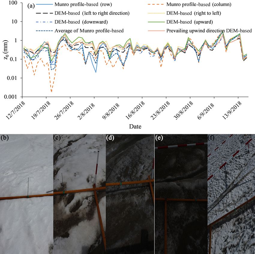
J. Liu et al.: Spatial and temporal variations in glacier aerodynamic surface roughness                                              969

Figure 1. Location of ice cap and study sites. (a) Location of the August-one glacier. (b) Locations of the AWS, automatic and manual
photogrammetry plots, and shortwave observation platforms.

Table 1. Measurement specifications for the AWS located at the top of the glacier (4820 m a.s.l.). The heights indicate the initial sensor
distances to the glacier surface; the actual distances are derived from the SR50A sensor.

                        Variable                     Sensors                 Stated accuracy    Initial height (m)
                        Air temperature              Vaisala HMP 155A        ±0.2 ◦ C           2, 4
                        Relative humidity            Vaisala HMP 155A        ±2 %               2, 4
                        Wind speed                   Young 05103             ±0.3 m s−1         2, 4
                        Wind direction               Young 05103             ±0.3◦              2, 4
                        Ice temperature              Apogee SI-11            ±0.2 ◦ C           2
                        Shortwave radiation          Kipp&Zonen CNR-4        ±10 % d total      2
                        Longwave radiation           Kipp&Zonen CNR-4        ±10 % d total      2
                        Surface elevation changes    Campbell SR50A          ±0.01 m            2
                        Precipitation                OTT Pluvio2             ±0.1 mm            1.7

moved along a 1.5 m long slider rail. The camera was 1.7 m             which took pictures of ice surface gauge stakes located near
above the ice surface and moved along the control frame.               the automatic photogrammetry site.
The seven pictures taken during this period were merged to
produce a picture of ice surface topography at millimeter              2.3   Manual photogrammetry
scale (Fig. 3b). This apparatus took pictures over a period
of 3 months (12 July to 15 September, the melting season).             Manual close-range photogrammetry was used to survey
A total of 64 d of data were recorded. Each daily photogra-            glacier surfaces at several different locations of the ice cap.
phy series produced four sets of pictures (12 h and 3 h inter-         Observations were made on 4 d: 12 and 25 July and 3 and
vals). The best-exposed photo sets were manually selected              28 August. It should be noted that when the July measure-
and used as that day’s data. We also set up instrumentation to         ments were performed, the ice cap surface was partially snow
record incoming and reflected solar radiation. Samples were            covered.
taken every 15 s; 10 min means were stored on a data logger               Channels account for only a small portion of the glacier
(CR800, Campbell, USA) located at a height of 1.5 m. Sur-              surface area. These surfaces show extreme variability of z0
face elevation changes caused by accumulation and ablation             (Rippin et al., 2015; Smith et al., 2016). For that reason,
were measured by a digital infrared hunting video camera,              we distributed the manual photogrammetry study sites over
                                                                       the glacier surface in such a way as to cover most surface

www.the-cryosphere.net/14/967/2020/                                                              The Cryosphere, 14, 967–984, 2020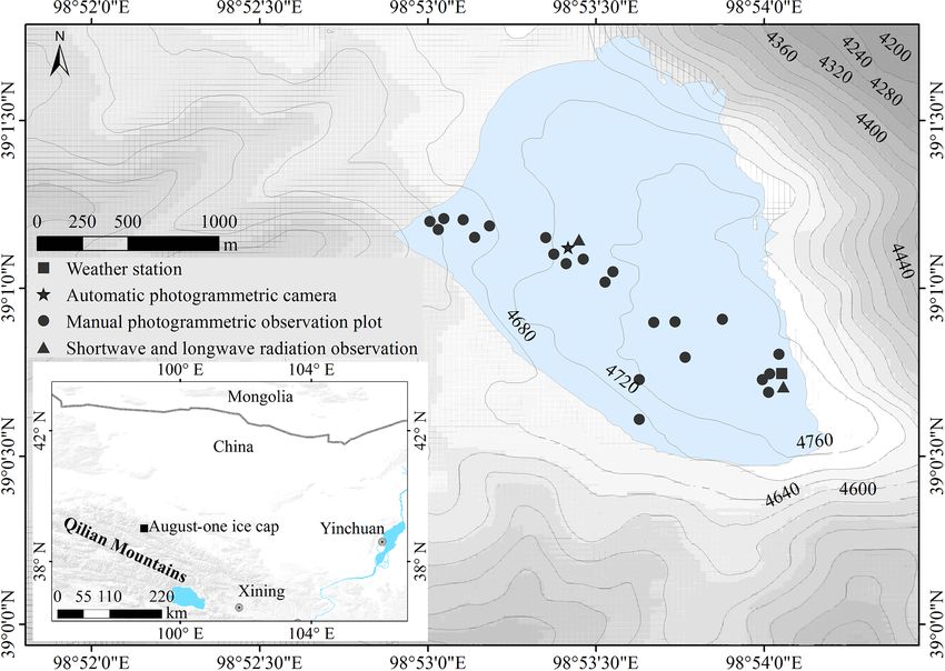
970                                J. Liu et al.: Spatial and temporal variations in glacier aerodynamic surface roughness

                                                                  imported into a software program, Agisoft Photoscan Pro-
                                                                  fessional 1.4.0. This software allowed us to estimate cam-
                                                                  era intrinsic parameters, camera positions, and scene geome-
                                                                  try. Agisoft Photoscan Professional is a commercial package,
                                                                  which implements all stages of photogrammetric processing
                                                                  (James et al., 2017). It has previously been used to generate
                                                                  three-dimensional point clouds and digital elevation models
                                                                  of debris-covered glaciers (Miles et al., 2017; Quincey et al.,
                                                                  2017; Steiner et al., 2018), ice surfaces and braided meltwa-
                                                                  ter rivers (Javernick et al., 2014; Smith et al., 2016). In our
                                                                  study, we found that after new snowfall it was difficult to
                                                                  match feature points in the photo sets. A total of 3 d of au-
                                                                  tomatic data could not be processed. We estimated z0 data
                                                                  for the missing days based on data from snowfall days at the
                                                                  automatic site.

                                                                  2.5    Aerodynamic roughness estimation

                                                                  Methods for measuring roughness at plot scale were first de-
                                                                  veloped by soil scientists (Dong et al., 1992; Smith, 2014).
                                                                  Metrics such as the random roughness (RR) or root-mean-
                                                                  square height deviation (σ ), the sum of the absolute slopes
                                                                  (6S), the microrelief index (MI) and the peak frequency
                                                                  (the number of elevation peaks per unit transect length) were
                                                                  used. Later these roughness indices were used to describe
                                                                  snow or ice surface roughness (Rees and Arnold, 2006; Fass-
                                                                  nacht et al., 2009b; Irvine-Fynn et al., 2014).
                                                                     Current photogrammetry methods produce high-
Figure 2. The automatic photogrammetry device at the August one
                                                                  resolution three-dimensional topographic data. Earlier
ice cap.
                                                                  two-dimensional profile-based methods for estimating
                                                                  surface roughness discard much of the potentially use-
                                                                  ful three-dimensional topographic data (Passalacqua et
types and topographic regions without including any chan-
                                                                  al., 2015). Smith et al. (2016) were able to use Eq. (1),
nels (Fig. 1b). We photographed a total of 36 sites over the
                                                                  developed by Lettau (1969), to make better use of the
4 d of observation.
                                                                  topographic data, using multiple point clouds and digital
   Study plots were demarcated with a 1.1 × 1.1 m portable
                                                                  elevation models (DEMs). Fitzpatrick et al. (2019) also
square aluminum frame. A geo-reference of the point cloud
                                                                  developed two methods for the remote estimation of z0 by
was enabled using control points established by eight cross-
                                                                  utilizing lidar-derived DEM. In this method, z0 is quantified
shaped screws on the aluminum frame (Fig. 3c). Photos (con-
                                                                  as follows:
vergent photographs, low oblique photos in which camera
axes converge toward one another) were taken at ∼ 1.6 m dis-                   s
                                                                  z0 = 0.5h∗ ,                                              (1)
tances, covering an area of ∼ 1.75 m2 . A total of 7 to 12 of                  S
such photos were taken at each survey site and surrounded
                                                                  where h∗ represents the effective obstacle height (m) and
the target area from different directions. The camera used
                                                                  is calculated as the average vertical extent of micro-
was an EOS 6D 50 mm, with a fixed focal lens and an im-
                                                                  topographic variations, s is the silhouette area facing up-
age size of 5472 × 3648 pixels. The f stop was fixed at f 22
                                                                  wind (m2 ), S is the unit ground area occupied by micro-
with an exposure time from 1/25 to 1/125 s.
                                                                  topographic obstacles (m2 ) and 0.5 is an averaged drag co-
                                                                  efficient.
2.4   Data processing
                                                                     Based on the work of Lettau (1969), Munro (1989) simpli-
Structure-from-motion photogrammetry is revolutionizing           fied Eq. (1) by assuming that h∗ can equal twice the standard
the collection of detailed topographic data (Westoby et al.,      deviation of elevations in the de-trended profile, with the pro-
2012; James et al., 2017). High-resolution DEMs produced          file’s mean elevation set to 0 m. The aerodynamic roughness
from photographs acquired with consumer cameras need              length for a given profile then becomes
careful handling (James and Robson, 2014). In this study,                f
both manual and automatically derived photographs were            z0 =     (σd )2 ,                                           (2)
                                                                         X

The Cryosphere, 14, 967–984, 2020                                                      www.the-cryosphere.net/14/967/2020/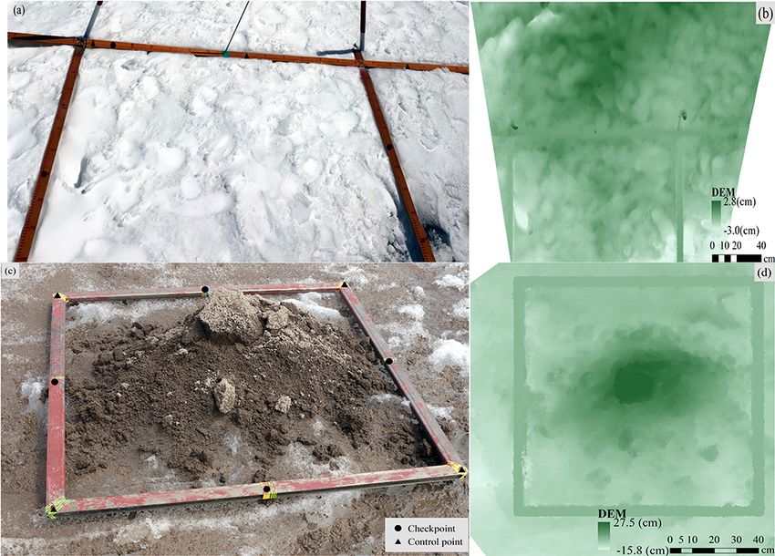
J. Liu et al.: Spatial and temporal variations in glacier aerodynamic surface roughness                                          971

Figure 3. Frames used for automatic and manual photogrammetry. (a) Wooden frame in situ set up for automatic photogrammetry; four
control points and three checkpoints are shown on the frame. (b) Detrended DEM for the corresponding snow surface of (a). (c) Manual
observation plot, with the four control points and four checkpoints shown on the aluminum frame. Ice surface hummock was covered with
cryoconites. (d) Detrended DEM for the corresponding cryoconite surface of (c).

where f is the number of up-crossings above the mean el-             was calculated for every profile (n = 1000) in both orthogo-
evation in profile, X is the length (m) of profile and σd is         nal directions for each plot at the automatic photogrammetry
the standard derivation of elevations of profile. For manual         site.
photogrammetry, we put the aluminum frame horizontally
over the ice surface, the plot is detrended by setting the con-      2.6   Snow and ice surface energy balance calculation
trol points at the z axis of the same values. For automatic
photogrammetry, the control field of wooden frame was also           The temporal variation in z0 at the automatic site was studied
laid horizontally over the ice surface, which lowered as the         from energy balance perspective. The surface heat balance of
ice melted and maintained a horizontal position between the          a melting glacier is given by
control field and ice surface. A DEM-based approach enables
the roughness frontal area s to be calculated directly for each      QM = Qis − Qos + QL + QE + QH + QP + QG ,                   (3)
cardinal wind direction (Smith et al., 2016). The combined
roughness frontal area was calculated across the plot, and           where QM is the heat flux of melting, Qis is the incoming
the ground area occupied by micro-topographic obstacles is           shortwave radiation, Qos is the outgoing shortwave radiation,
1 m2 . We used a DEM-based average (z0_DEM ) of the four             QL is the net longwave radiation, QE is the latent heat flux;
cardinal wind directions to represent overall aerodynamic            QH is the sensible heat flux, QP is the heat from rain and
surface roughness. Based on the 30 min wind direction data           QG is subsurface heat flux.
at the August one ice cap, the daily upward wind direction              In a horizontally homogeneous and steady surface state,
DEM-based z0_DEM was also estimated at the automatic pho-            the surface heat fluxes QE and QH can be calculated us-
togrammetry site. Considering that wind direction changed            ing either the bulk aerodynamic approach or profile method,
during the day, in this case we selected the prevailing wind         based on the Monin–Obukhov similarity theory (e.g., Arck
direction to calculate frontal area s. The prevailing upwind         and Scherer, 2002; Garratt, 1992; Oke, 1987). In this study,
direction DEM-based z0_DEM was applied to calculate tur-             30 min observations at 4 m level and daily upward wind di-
bulent heat flux. Using the Munro (1989) method, z0_profile          rection DEM-based z0 were used to calculate QE and QH
                                                                     based on the bulk method. The heat from rain is given by

www.the-cryosphere.net/14/967/2020/                                                          The Cryosphere, 14, 967–984, 2020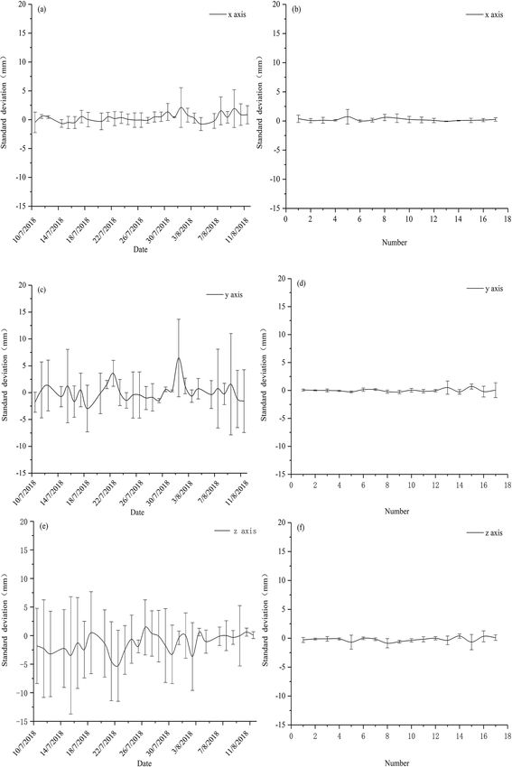
972                                 J. Liu et al.: Spatial and temporal variations in glacier aerodynamic surface roughness

Table 2. Control point RMSE for manual and automatic photogrammetry

                       Ground control points    x error (mm)     y error (mm)    z error (mm)     Total error (mm)
                       Automatic     Point 1            0.71              5.83          6.61                 5.11
                                     Point 2            0.41              1.14          0.74                 0.82
                                     Point 3            0.54              4.55          2.40                 2.99
                                     Point 4            0.45              0.76          1.04                 0.79
                                     Average            0.54              3.76          3.58                 3.01
                       Manual        Point 2            0.62              0.43          0.81                 1.11
                                     Point 4            0.44              0.27          0.43                 0.67
                                     Point 5            0.18              0.47          0.85                 0.99
                                     Point 7            0.66              0.39          2.97                 3.07
                                     Average            0.52              0.40          1.65                 1.78

Table 3. Checkpoint RMSE for manual and automatic photogrammetry.

                       Ground checkpoints       x error (mm)     y error (mm)    z error (mm)     Total error (mm)
                       Automatic     Point 5            2.06              4.44          7.70                 5.27
                                     Point 6            0.91              3.56          1.95                 2.40
                                     Point 7            0.98              3.11          2.60                 2.41
                                     Average            1.41              3.74          4.83                 3.62
                       Manual        Point 1            0.30              0.19          0.39                 0.52
                                     Point 3            0.79              0.37          0.69                 1.12
                                     Point 6            0.28              0.83          0.90                 1.26
                                     Point8             0.46              0.45          0.44                 0.77
                                     Average            0.52              0.53          0.66                 0.99

Konya and Matsumoto (2010):                                           3     Results

QP = ρw CW TW Pr ,                                             (4)    3.1    Photogrammetry precision

where ρw is the density of water (1000 kg m−3 ), CW is                We used 17 plots to analyze the horizontal and vertical ac-
the specific heat of water (4187.6 J kg−1 K−1 ), TW is the            curacy of our automatic photogrammetry and 31 plots for
wet-bulb temperature (K) and Pr is the rainfall intensity             our manual photogrammetry. Based on the Agisoft Pho-
(mm). The subsurface heat flux QG is estimated from the               toscan processing report, automatic photogrammetry aver-
                                                            ∂t 0
temperature–depth profile and is given by QG = −kT ∂z          0,     age point density of the final plot point clouds was over
where kT is the thermal conductivity, i.e., 0.4 Wm−1 K−1 for          1 000 000 points m−2 . DEMs of 1 mm resolution were gener-
old snow and 2.2 W m−1 K−1 for pure ice (Oke, 1987).                  ated at plot scale. The average geo-reference errors fluctuated
   In order to calculate Pr , we used the air temperatures            at around 1 mm (see Tables 2 and 3). Total root-mean-square
recorded at the AWS. There is an elevation difference be-             error (RMSE) of the automatic control points was 3.0 ±
tween the study site (4700 m) and the AWS (4790 m).                   2.1 mm and for the checkpoints it was 3.62 ± 1.6 mm. Ver-
Recorded air temperatures were corrected to account for the           tical error for control points was 3.58 mm ± 3.01 mm and for
elevation difference. A lapse rate of −5.6 ◦ C km−1 was ap-           the checkpoints it was 4.83 ± 2.9 mm (Tables 2 and 3). Stan-
plied based on observations made nearby (Chen et al., 2014).          dard deviation of control and checkpoint errors are all within
The ice cap is flat and open terrain so in this case wind speed       15 mm (Fig. 4a, c, e). Manually measured average point den-
and relative humidity at the study sites were assumed to be           sity of the final plot point clouds was > 6 000 000 points m−2 .
close to those observed at the AWS.                                   DEM of 1 mm resolution was generated at plot scale. The
                                                                      RMSE of four control points is 1.78 ± 1.3 mm (Table 1). The
                                                                      control point vertical accuracy of manual photogrammetry is
                                                                      about 1.65±1.3 mm. The total RMSE of manual photogram-
                                                                      metry checkpoints is 0.99±0.3 mm and the vertical accuracy
                                                                      is 0.66 ± 0.3 mm (see Tables 2 and 3). Standard deviation for
                                                                      the x, y and z axes were all within 5 mm (Fig. 4b, d, f).

The Cryosphere, 14, 967–984, 2020                                                               www.the-cryosphere.net/14/967/2020/
J. Liu et al.: Spatial and temporal variations in glacier aerodynamic surface roughness 973 Figure 4. Automatic and manual photogrammetry checkpoint errors. Panels (a), (c) and (e) are automatic photogrammetry standard deviation for the x, y and z axes, respectively. Panels (b), (d) and (f) are manual photogrammetry standard deviation for the x, y and z axes, respectively. www.the-cryosphere.net/14/967/2020/ The Cryosphere, 14, 967–984, 2020
974                                 J. Liu et al.: Spatial and temporal variations in glacier aerodynamic surface roughness

Figure 5. (a) Variation in glacier surface aerodynamic roughness over time at the automatic observation site for the DEM-based and Munro
(1989) profile-based approaches. Panel (b) shows a snow-covered surface on 13 July. Panel (c) shows a partially snow-covered surface on
23 July with cryoconite holes. Panels (d) and (e) show a smooth ice surface on 1 and 30 August. Panel (f) shows a rough ice surface on
13 September.

   Note that the control and checkpoint errors are larger for         3.2   Aerodynamic surface roughness as measured by
the automatic measurements than for the manual ones (see                    automatic photogrammetry
Fig. 4). We believe that this is the case because, rather than
using static f stop and exposure times (as in automatic pho-          Data for ice surface roughness was collected by the automatic
togrammetry), researchers engaged in manual photogramme-              photogrammetry camera site from 12 July to 15 Septem-
try could adjust exposure time based on ice surface condi-            ber, a period covering the whole melting season. Profile and
tions. This allowed production of better quality photos even          DEM data show that z0 estimates vary by 2 orders of magni-
on cloudy or foggy days. This difference in survey design             tude over the study period (Fig. 5). The upwind DEM-based
also caused more precise results for manual than automatic            data showed a z0_DEM varying from 0.1 to 1.99 mm (mean:
photogrammetry. For the automatic measurements, the cam-              0.55 mm). The average of the four cardinal wind directions’
era was moving linearly and the density of tie points was             DEM data shows a z0_DEM varying from 0.1 to 2.55 mm
much higher in the foreground compared to the background.             (mean: 0.57 mm). The average Munro profile-based z0_profile
For the manual method, photos were taken by surrounding               varied from 0.03 to 2.74 mm (mean 0.46 mm).
the target area. This type of surface provided a much more               At the start of the observation period of 12 July, snow
robust elevation model and point density.                             covered the study site. As the snow melted, the ice cap sur-
                                                                      face z0 increased. During this period, z0 dropped to around
                                                                      0.1 mm due to intermittent snowfall. On 21 July, cryoconites
                                                                      appeared on patches of snow crust, which led to patchy melt.
                                                                      From 21 to 24 July, overall z0_DEM increased from 0.1 to
                                                                      1.6 mm. By 29 July, snow had disappeared from the study

The Cryosphere, 14, 967–984, 2020                                                            www.the-cryosphere.net/14/967/2020/
J. Liu et al.: Spatial and temporal variations in glacier aerodynamic surface roughness 975
Figure 6. Surface roughness vs. altitude, (a) as observed on 12 July, (b) 25 July, (c) 3 August and (d) 28 August.
site, and z0 fluctuated but trended lower. From 29 July to surfaces featured cryoconite holes and snow crust. Both the
5 August bare ice covered the whole field of view; z0_DEM automatic and manual observations showed the same pattern:
ranged from 0.18 to 0.56 mm. From 6 August to 3 Septem- maximum z0 at the snow–ice transition belt during partially
ber there was intermittent snowfall followed by melting, and snow-covered periods.
z0_DEM ranged from 0.1 to 1.0 mm. From 4 to 14 Septem-
ber z0_DEM showed an overall increase, reaching a maximum 3.3 Surface roughness as measured by manual
of 2.55 mm on 8 September. There was intermittent snow- photogrammetry
fall during this period, which temporarily reduced z0_DEM ,
which then increased thanks to patchy microscale melting. No wind direction measurements were carried out during
After 14 September, snow covered the whole surface of the manual photogrammetry. In this case, we presented an av-
glacier and there was no melting and little fluctuation in z0 . erage of the four cardinal directions to represent ice aero-
It should be clear that either z0_profile or z0_DEM and dynamic surface roughness. Analysis indicated that z0_DEM
z0_DEM varied following the same pattern during the melt- proved to have an interesting relationship with altitude.
ing season. There were two peaks in z0 , both of which oc- z0_DEM was highest in the transition zone between snow
curred in periods of transition: snow surface turning to ice cover and ice. This zone moved up the ice cap during the
around 24 July and ice surface turning to snow on 8 Septem- melting season. On 12 July, ice surface roughness decreased
ber. On 24 July and again on 8 and 13 September, glacier from 3.2 to 0.25 mm as altitude increased (Fig. 6a; r =
0.8429; P = 0.0006 < 0.01). Near the ice cap terminals at
www.the-cryosphere.net/14/967/2020/ The Cryosphere, 14, 967–984, 2020976 J. Liu et al.: Spatial and temporal variations in glacier aerodynamic surface roughness
Figure 7. Weather conditions at AWS over study period: (a) precipitation, (b) air temperature, (c) incident solar radiation, (d) relative
humidity and (e) wind speed.
4590 m, the ice surface featured porous snow and ice and ice cap surface roughness showed no significant correlation
many cryoconite holes. As altitude increased, the number with altitude (Fig. 6d, r = −0.03). z0_DEM varied from 0.2 to
of cryoconite holes decreased and snow coverage increased. 0.98 mm (Fig. 6d). When we compare the results of the four
At 4700 m the ice surface was predominantly snow covered surveys, we see that ice surface roughness was variable. Max-
and only a few small patches were free of snow. On 25 July, imum z0 was seen at the snow and ice transition zone, where
ice surface roughness fluctuated between 0.27 to 0.65 mm at the ice surface featured both cryoconite holes and clean snow
the ice cap terminals (4593 m). At ∼ 4700 m, roughness in- crust. Snow crust would have inhibited melting; cryoconite
creased to 1.85 mm. Above that point, roughness gradually would have increased it. It is thus understandable that surface
decreased to 0.25 mm at the ice cap top, which was covered roughness would have been greater in such an area. Bare ice
by snow (Fig. 6b). or snow cover both result in comparatively less roughness.
On 3 August, the August one ice cap was predominantly
bare ice and there was scattered snow crust at the ice cap 3.4 z0 and weather
top. The ice surface (terminal to top) showed a heavy de-
posit of cryoconite. Photogrammetric data collected manu-
Figure 7 compared z0_DEM and corresponding meteorolog-
ally revealed that ice surface roughness increased with alti-
ical conditions of precipitation, air temperature, downward
tude (Fig. 6c, r = 0.7). From the terminals to the top of the
solar radiation, relative humidity and wind speed. Detailed
ice cap, z0 varied from 0.06 to 2.2 mm. On 29 August, the
analysis indicates snowfall was recorded from 12 to 24 July.
The Cryosphere, 14, 967–984, 2020 www.the-cryosphere.net/14/967/2020/J. Liu et al.: Spatial and temporal variations in glacier aerodynamic surface roughness 977
In general, snowfall reduced roughness if it resulted in a fully
snow-covered surface. However, if a patchy, shallow snow
cover was formed, it tended to increase z0 after a short drop.
For example, on 11 and 12 August, two successive sleety
days created a patchy snow cover which soon increased z0 .
Between 26 July and 31 August there were 16 rainfall events,
which tended to lower ice surface z0 .
Daily temperatures during the study period ranged from
−6.5 to 7.1 ◦ C (mean: 1.3; Fig. 7c). It was 1.2 ◦ C on 11 July.
It increased to 3.6 ◦ C on 24 July (the date when z0 was high-
est). It continued increasing until 29 July, when it reached its
highest annual of 7.1 ◦ C. During this period z0 continuously
declined. From 28 July to the end of August temperatures Figure 8. Daily mean energy balance at the middle of the glacier
fluctuated between −0.3 and 5.7 ◦ C with no evident trend. study site, which was close to the automatic photogrammetry site.
z0_DEM also fluctuated slightly, showing no obvious trend.
In September air temperature quickly dropped from 0.6 to
−6.5 ◦ C. There were large fluctuations in z0 during this pe- ergy flux. Latent heat was generally small throughout the
riod. The largest fluctuations appeared when air temperatures study period. Daily mean of latent heat varied from −80.1
dropped from positive to negative. to 11.1 W m−2 (mean: −13.2 W m−2 ). It accounts for a mere
Daily downward mean solar radiation fluctuated dramati- 0.9 % for the total incoming flux. It was negative from 11 to
cally during the study period due to cloudy and overcast con- 26 July when the ice surface was snow covered. After 26 July
ditions (Fig. 7d). Incident solar radiation fluctuated between the latent heat was mainly positive in the following 10 d (the
129 and 753 W m−2 (mean: 469 W m−2 ). From 29 July to ice surface was pure ice or partially snow covered). From
the end of August, the weather was cloudy, warm, calm, and 6 August to the end of the study period (15 September) it
humid most of the time (Fig. 7b, c, e, f) and z0_DEM was rel- was predominantly negative.
atively stable, except when there was intermittent snowfall- From 25 July to 5 August rainfall energy varied from 0
induced fluctuation. After September, the weather again be- to 11.7 W m−2 (mean: 0.3 W m−2 ). Rainfall accounted for a
came cold and dry and z0 was quite variable. mere 0.2 % of total incoming flux. One event accounted for
much of the total: on 28 July a 31 mm rainfall event added
3.5 Ice surface energy balance at automatic z0 a flux of 11.7 W m−2 , which resulted in visible smooth-
observation study site ing of the ice surface (Fig. 9). Compared to other energy
components, QG was very small, with a daily mean of
The following section analyzes the changes in surface en- −0.65 W m−2 and a maximum and minimum of −0.4 and
ergy balance at the automatic site. Meteorological obser- −2.1 W m−2 , respectively.
vation records allowed us to study the factors that control
ice surface roughness. Net radiation varied from −9.7 to 3.6 Modeled vs. observed surface ablation
260.2 W m−2 (mean: 95.3 W m−2 ) during the study period.
This constituted the largest energy flux affecting glacier sur- Based on the previously listed measurements of energy
face energy balance. It accounted for 84 % of total incom- fluxes, we calculated the probable surface ablation at the au-
ing flux (Fig. 8). Net radiation was relatively low in the tomatic photogrammetry site. We took into account observed
first 13 d of the study period (mean: 69.3 W m−2 ), when the net radiation, bulk-method-calculated turbulent heat fluxes,
glacier surface was covered with snow. In the succeeding 5 d, heat from rainfall and subsurface heat flux. There was good
net radiation increased to 103.9 W m−2 . At this time the ice agreement between the model and observed results (Fig. 10).
surface exhibited a patchwork of snow, ice, and cryoconite. Figure 11 shows the relationship between estimated daily
From 29 July to 5 August the surface of the study site was upward wind direction DEM-based z0_DEM and the main en-
composed of ice with a dusting of cryoconite. Net radia- ergy flows. Scatter diagrams showed a positive relationship
tion reached a height of 183 W m−2 . There was intermit- between z0_DEM and net shortwave radiation (Fig. 11a, r =
tent snowfall from 6 August to 8 September. Net radiation 0.1) and a significant negative relationship between z0_DEM
dropped to a mean 93 W m−2 . Snow cover then appeared and and net longwave radiation (Fig. 11b, r = −0.35), Graph-
net radiation dropped to a low of 46 W m−2 . ing z0_DEM vs. bulk-method-estimated latent heat showed a
Bulk-method-estimated results indicate that sensible heat significant negative exponential relationship (Fig. 11d, r =
(QH ) was the second largest energy flux component of in −0.35). The scatter diagram showed no significant relation-
surface energy balance during the study period (Fig. 8). The ship between z0_DEM and the bulk-method-estimated sensi-
sensible heat daily mean varied from −7.1 to 66.3 W m−2 . It ble heat (Fig. 11c). The average of the Munro profile-based
accounted for −28 % to 32 % (mean: 15 %) of the net en- z0_profile , DEM-based z0_DEM and the main energy items are
www.the-cryosphere.net/14/967/2020/ The Cryosphere, 14, 967–984, 2020978 J. Liu et al.: Spatial and temporal variations in glacier aerodynamic surface roughness
Figure 9. Ice surface overview at the automatic photogrammetry site before and after a strong rainfall event captured by an automatic digital
infrared hunting video camera: (a) photograph taken before the rainfall event on 4 August of 2018 and (b) photograph taken after the strong
rainfall event on 5 August of 2018.
Table 4. The lagged correlation between z0 and the main energy
items during the melting season; the sensible heat and latent heat
were calculated here based on the bulk method.
z0_profile n (Qis − Qos ) QL QE QH LS
Lag 0 64 0.143 −0.309∗ −0.614∗ −0.088 −0.578∗
Lag 1 63 0.131 −0.346∗ −0.646∗ −0.137 −0.572∗
Lag 2 62 −0.022 −0.113 −0.356∗ −0.307∗ −0.585∗
Lag 3 61 −0.144 0.051 −0.193∗ −0.283∗ −0.523∗
Lag 4 60 −0.142 −0.241 −0.016 −0.013 −0.205
n = the number of samples, ∗ P < 0.05.
Because net shortwave radiation and turbulent heat fluxes
were the main energy fluxes affecting ice surface roughness,
we calculated a turbulent heat proportion index:
LS = (QH + QE + QP )/(Qis − Qos ). (5)
Note that aerodynamic surface roughness on days when snow
fell was strongly affected by the amount of the snowfall.
Figure 10. Comparison of observed daily mass balance and mod- If we exclude snowfall days and snow-covered period, we
eled daily mass balance. Mass balance measurements were taken see a significant exponential relationship between ice surface
from 12 July to 29 August. Measurements of surface lowering were z0_DEM and LS (Fig. 12a, r = −0.34). The scatter diagrams
converted into water equivalents using density values. showed a significant exponential relationship between ice
surface z0_profile and LS and net longwave radiation (Fig. 12c,
r = −0.69). z0_DEM vs. LS also showed a significant expo-
also analyzed. Scatter diagrams showed a significant nega-
nential relationship (Fig. 12b, r = −0.46). Scatter diagrams
tive relationship between z0_profile and net longwave radiation
in Fig. 12 also showed z0 did not keep decreasing when LS
(Fig. S1a, r = −0.5). Graphing z0_profile vs. the bulk-method-
was above 0.2. z0_DEM , z0_profile and z0_DEM were around
estimated latent heat showed a significant negative exponen-
0.56 ± 0.21, 0.33 ± 0.03 and 0.6 ± 0.26 mm, respectively.
tial relationship (Fig. S1d, r = −0.69). The scatter diagram
The z0 (z0_DEM and z0_profile z0_DEM ) vs. LS graph indi-
showed no significant relationship between z0_profile and the
cates that when turbulence and rainfall heat increased, aero-
bulk-method-estimated sensible heat (Fig. S1c). z0_DEM vs.
dynamic surface roughness decreased. As soon as LS is
the bulk-method-estimated latent heat showed a significant
above 0.2, the ice surface will not keep smoothing and z0
negative exponential relationship (Fig. S2d, r = −0.44). In
sustains its lowest stage. Time series correlation of all main
the scatter diagrams between z0_DEM and net shortwave ra-
energy items and z0_profile were performed. Table 4 shows
diation, the bulk-method-estimated sensible heat showed no
an example of the lagged correlations between z0_profile and
significant relationship.
five variables. The z0 and net shortwave radiation displayed a
positive correlation with 0 to 1 d lag time. The z0 response to
The Cryosphere, 14, 967–984, 2020 www.the-cryosphere.net/14/967/2020/J. Liu et al.: Spatial and temporal variations in glacier aerodynamic surface roughness 979
Figure 11. Daily upward wind direction of DEM-based z0_DEM vs. energy inputs: (a) z0_DEM vs. net shortwave radiation, (b) z0_DEM vs.
net longwave radiation, (c) z0_DEM vs. bulk-method-calculated sensible heat and (d) z0_DEM vs. bulk-method-calculated latent heat.
QE with a correlation of −0.6 showed a lag of 0 to 1 d. The 4 Discussion
z0_profile also had a negative relationship with QL with no lag
or 1 d lag time. The z0_profile response to LS with a correla- 4.1 Automatic and manual photogrammetric methods
tion of −0.58 was with a lag of 0 to 2 d. A total of 0 to 2 d lag
time gives an indication of the effort limitations of the main Photogrammetric techniques such as Structure from Mo-
energy items over ice surface z0 . In other words, a sunny tion (SfM) (James and Robson, 2012) and Multi-view
and cold day facilitates rough ice surfaces and warm and Stereo (MVS) represent low-cost options for acquiring high-
cloudy days tend to produce a smoother ice surface. When resolution topographic data. Such approaches require rela-
net shortwave radiation is higher and latent and sensible heat tively little training and are extremely inexpensive (Westoby
are smaller, z0 tends to be higher for the next 2 d. When net et al., 2012; Fonstad et al., 2013; Passalacqua et al., 2015).
shortwave radiation is smaller, as on cloudy days, any snow- We used both automatic and manual photogrammetric meth-
fall or rainfall is usually associated with smaller z0 for the ods to sample spatial and temporal z0 variation at the August
following 2 d. Under a negative QM , the surface z0 would one ice cap. Adjustments to exposure time based on ice sur-
not be affected by melting process. face conditions and survey design of the area surrounding the
target made the manual photogrammetry more precise than
automatic photogrammetry (Tables 2 and 3). However, preci-
sion is not always the major concern. The glacier surface was
a harsh (even punishing) environment for the researchers do-
www.the-cryosphere.net/14/967/2020/ The Cryosphere, 14, 967–984, 2020980 J. Liu et al.: Spatial and temporal variations in glacier aerodynamic surface roughness
Figure 12. Aerodynamic surface roughness vs. LS . Where LS = (QH + QE + QP )/(Qis − Qos ), in (a) z0_DEM was estimated based on
DEM-based prevailing upwind direction, in (b) z0_DEM was the average of the four cardinal wind directions’ z0 in order to represent overall
aerodynamic surface roughness and in (c) z0_profile was the average of two orthogonal directions z0 .
ing manual photogrammetry. In addition, manual photogram- turbulent fluxes. The transition zone had maximum z0 , and
metry took much longer. Automatic methods reduced hours the zone also migrated across much of the glacier, highlight-
of field work, spared researchers and produced nearly contin- ing the importance of transient surface characteristics.
uous data. Cloudy or frosty weather affected automatic pho- Micro-topography, wind profile and eddy covariance
togrammetry exposures, and heavy snowfalls resulted in a methods generate a wide range of z0 values for snow and ice
textureless surface. Nevertheless, it is likely that photogram- surfaces (Grainger and Lister, 1966; Munro, 1989; Bintanja
metry techniques will continue to improve and that these and Broeke, 1995; Schneider, 1999; Hock and Holmgren,
drawbacks may be mitigated. 2005; Brock et al., 2006; Andreas et al., 2010; Gromke et
al., 2011). In this study, z0_profile , z0_DEM and z0_DEM showed
4.2 Spatial and temporal variability of z0 similar variation pattern during the melting season. The dif-
ference of z0_profile , z0_DEM , and z0_DEM were within 1 or-
Previous studies of glacier surfaces roughness have rarely der of magnitude. The latent and sensible heat calculated
covered the whole glacier, from the terminals to the top of by z0_profile , z0_DEM and z0_DEM were highly relevant among
the ice cap, in one melting season (Föhn, 1973; Smeets et al., these methods. The automatic photogrammetry estimated z0
1999; Denby and Smeets, 2000; Greuell and Smeets, 2001; for snow-covered surfaces ranged from 0.1 to 0.55. New
Albert and Hawley, 2002; Brock et al., 2006; Smeets and Van snowfall at the snow surface in July formed the lowest z0
den Broeke, 2008; Smith et al., 2016). This whole-glacier values. Previous studies have shown that freshly fallen snow
study allowed us to follow the movement of the transition is subject to rapid destructive metamorphism (McClung and
zone, where snow was melting and exposing ice, from the Schaerer, 2006), which can dramatically change the rough-
terminals to the top of the ice cap. The transition zone moved ness of fresh snow surfaces (Fassnacht et al., 2009b). Our
up as the melting season proceeded, thus roughening the sur- study showed that z0 followed an increasing trend during the
face of the glacier and raising z0 . At the start of the melt- melting season. Intermittent snowfall first decreased snow
ing season, snow cover first disappeared, leaving an ice sur- surface z0 , which then began to increase as the snow sur-
face at the terminal end of the August one ice cap, i.e., at the face deteriorated. In the data from Clifton et al. (2008),
lower altitude. This newly exposed surface was rougher (z0 snow surface z0 was estimated at between 0.17 to 0.6 mm
was higher) than on the upper part of glacier, which was still in a wind tunnel experiment. In an analysis of ultrasonic
snow covered (see the black line in Fig. 6a for z0 distribution anemometer recorder data over snow-covered sea ice, An-
at different altitudes). As the snowline shifted to higher alti- dreas et al. (2010) found z0 values ranging from 10−2 to
tudes, ice surface increased, as did z0 (see the dashed black 101 mm. In a wind tunnel experiment of fresh snow with no-
curve in Fig. 6b). As the melting continued, the snow and drift conditions, Gromke et al. (2011) estimated z0 to be be-
ice transition belt reached the top of glacier (see the dotted tween 0.17 to 0.33 mm, with no apparent dependency on the
curve in Figure 6c). When the ice cap was completely free friction velocity. Our snow surface data showed that z0 values
of snow, z0 and elevation were no longer correlated (see the fluctuated between 0.03 to 0.55 mm, consistent with some of
dotted–dashed line in Fig. 6d). In summary, maximum z0 was those wind tunnel studies. The scatter of z0 data reported in
recorded at the cross-glacier transition zone between snow some studies is quite large, with a range of 10−2 to 101 mm.
and ice. This zone shifted from lower altitude to higher alti- The result may be attributed to the occurrence of snow drift, a
tude, from the terminals to the top of the ice cap, during the transitional rough-flow regime and large uncertainties in the
melting season. The spatial pattern of z0 distribution affected
The Cryosphere, 14, 967–984, 2020 www.the-cryosphere.net/14/967/2020/J. Liu et al.: Spatial and temporal variations in glacier aerodynamic surface roughness 981
estimation of friction velocities that propagate to the compu- smoothing process makes ice surface z0 fluctuate at around
tation of z0 (Andreas et al., 2010; Gromke et al., 2011). In 0.56 mm as long as the air temperature is above 0 ◦ C. When
contrast, the small scatter in our data was induced only by the temperature drops below 0 ◦ C, bright sunlight and dry
the natural variability of snow surface roughness. weather shutdown the ice surface smoothing process. The
For patchy snow-covered ice surfaces, z0 varied from 0.5 shortwave radiation induces even rougher ice and larger z0
to 2.6 mm and ice surface z0 varied from 0.24 to 1.1 mm. until snow covers the ice surface. At the August one ice cap,
During the melting season, there were no blowing snow the turbulent heat contributes a small portion of incoming en-
events and snow surface z0 was relatively smaller than in ergy, but the smoothing ice surface process decreases ice sur-
patchy snow-covered surface or ice surface. Ice surface z0 face albedo and seems to enhance ice surface shortwave ra-
was generally larger than snow surface and smaller than diation. The z0 fluctuation in the melt season is similar, with
patch snow-covered surface. Our results match values re- cryoconite holes developing when the radiative flux is dom-
ported in studies reporting results ranging from 0.1 to 6.9 mm inant and decaying when turbulent heat is dominant (McIn-
in Qilian mountain glaciers (Guo et al., 2018; Sun et al., tyre, 1984; Takeuchi et al., 2018). The glacier surface energy
2018). Our results showed that z0 reached its maximum at the balance components vs. z0 analysis in this study confirm that
end of the summer melt, which matched wind profile mea- the main energy items of net shortwave radiation and turbu-
surements by Smeets and Broeke (2008). lent heat flux affect the same-day z0 and following 2 d of z0 .
The aerodynamic surface roughness is influenced by both This study found an exponential relationship between z0 and
the boundary layer and the surface. In this study, the micro- LS . The delicate role of z0 played in the ice surface balance is
topographic estimated aerodynamic surface roughness only still not fully known. Further comparative studies are needed
considers surface topography at plot scale but its variability to investigate the z0 variation through eddy covariance and
is influenced by its surrounding topography and the boundary profiling methods and DEM-based z0 estimation.
layer. Thus, the results of z0 estimated in this study still need
to be validated by wind tower or eddy covariance observa-
tions. However, micro-topographic roughness metrics are a 5 Conclusions
very strong proxy for z0 (e.g., Nield et al., 2013), so we have
much more confidence in the temporal and spatial variability Manual and automatic measurements of snow and ice surface
presented by this work. roughness at the August one ice cap showed spatial and tem-
poral variation in z0 over the melting season. Manual mea-
4.3 Effects of surface energy balance components on surements, taken from the terminals to the top of the ice cap,
aerodynamic surface roughness show that the nature of the surface cover features are corre-
lated with z0 rank in the following order: transition region >
Aerodynamic roughness is associated with the geometry of pure ice area or pure snow area. The transition region forms
ice roughness elements (Kuipers, 1957; Lettau, 1969; Munro, a zone of maximum z0 , which shifts over the melting season
1989). Surface geometry roughness develops due to local from the terminals to the top of the ice cap. The observed z0
melt inhomogeneities in melting season. In earlier works, re- vs. energy items analysis indicated that LS (turbulent heat in-
searchers argued that a variety of ablation forms, such as sun dex) was also an important determinant of ice aerodynamic
cups, penitents, cryoconite holes or dirt cones, are formed surface roughness.
by the sun (Matthes, 1934; Lliboutry, 1954; McIntyre, 1984; Aerodynamic surface roughness is a major parameter in
Rhodes et al., 1987; Betterton, 2000). These ablation forms calculations of glacier surface turbulent heat fluxes. In pre-
develop in regions with bright sunlight and cold, dry weather vious studies investigators used a constant z0 value for the
conditions are apparently required (Rhodes et al., 1987). whole surface of the glacier. This study captures a much
These structures are observed to decay if the weather is smaller-scale variation in spatial and temporal glacier surface
cloudy or very windy (Matthes, 1934; Lliboutry, 1954; McIn- aerodynamic roughness through automatic and manual pho-
tyre, 1984). togrammetric observations. Such close observation of vari-
The August one ice cap dust concentrations are high in the ation in z0 certainly enhanced the accuracy of the surface
melting season. Cryoconites are unevenly distributed over energy balance models developed in the course of this study.
the ice surface, leading to differential absorption of short- This study was carried out at an ice cap with a neat or-
wave radiation at microscale. This process results in the dering of its annual layers. The August one ice cap moved
roughening of the ice surface, a process that enhances turbu- slowly, no crevasses were formed over the ice cap and chan-
lent heat exchange across the atmospheric boundary layer– nels were not considered in this study. In this case, a more
ice interface. When the air temperature is above 0 ◦ C, the moderate variation in z0 was estimated than would be found
ice surface keeps melting. The turbulent heat smooths the ice for debris-covered glaciers (Miles et al., 2017; Quincey et
surface, increases the cryoconite concentration over the ice al., 2017). Uneven or heterogeneous ice surfaces such as sas-
surface and decreases ice surface albedo, enhancing short- trugi, crevasses, channels and penitents could greatly affect
wave radiation absorption (Fig. 9). This roughening and ice surface aerodynamic surface roughness, and it would be
www.the-cryosphere.net/14/967/2020/ The Cryosphere, 14, 967–984, 2020982 J. Liu et al.: Spatial and temporal variations in glacier aerodynamic surface roughness
hard to estimate its z0 based on a profile method. SfM esti- Bintanja, R. and Van den Broeke, M.: Momentum and
mation of z0 might be a good choice at a macroscale. In the scalar transfer-coefficients over aerodynamically smooth
accumulation season, more attention would need to be paid Antarctic surfaces, Bound.-Lay. Meteorol., 74, 89–111,
to spatial and temporal variations in z0 , as z0 is a key pa- doi:10.1007/BF00715712, 1995.
rameter for sublimation calculation during this period. Stud- Brock, B. W., Willis, I. C., and Sharp, M. J.: Measurement and
parameterization of aerodynamic roughness length variations at
ies have indicated that the Lettau (1969) approach calculated
Haut Glacier d’Arolla, Switzerland, J. Glaciol., 52, 1–17, 2006.
z0 dependent on plot scale and resolution. In this study, we Chen, R. S., Song, Y. X., Kang, E. S., Han, C. T., Liu, J. F., Yang, Y.,
only select 1 m×1 m scale at 1 mm resolution to study spa- Qing, W. W., and Liu, Z. W.: A Cryosphere-Hydrology Observa-
tial and temporal variability. Further comparative studies of tion System in a Small Alpine Watershed in the Qilian Moun-
z0 are needed at different scales and resolutions. tains of China and Its Meteorological Gradient, Arct. Antarct.
Alp. Res., 46, 505–523, doi:10.1657/1938-4262-46.2.505, 2014.
Clifton, A., Manes, C., Rueedi, J. D., Guala, M., and Lehning,
Data availability. All of the observation and model input and out- M.: On shear-driven ventilation of snow, Bound.-Lay. Meteorol.,
put data presented in this study are available upon request to the 126, 249–261, doi:10.1007/s10546-007-9235-0, 2008.
corresponding author (Rensheng Chen, crs2008@lzb.ac.cn). Denby, B. and Smeets, C.: Derivation of turbulent flux profiles and
roughness lengths from katabatic flow dynamics, J. Appl. Mete-
orol., 39, 1601–1612, 2000.
Author contributions. JL and RC designed the study and wrote the Denby, B. and Snellen, H.: A comparison of surface renewal theory
paper. JL and CH carried out field-based manual photogrammetry with the observed roughness length for temperature on a melting
observations. glacier surface, Bound.-Lay. Meteorol., 103, 459–468, 2002.
Dong, W. P., Sullivan, P. J., and Stout, K. J.: Comprehensive study of
parameters for characterizing three-dimensional surface topog-
Competing interests. The authors declare that they have no conflict raphy I: Some inherent properties of parameter variation, Wear,
of interest. 159, 161–171, 1992.
Fassnacht, S. R., Stednick, J. D., Deems, J. S., and Cor-
rao, M. V.: Metrics for assessing snow surface roughness
from digital imagery, Water Resour. Res., 45, W00D31,
Acknowledgements. We thank the editor and the two reviewers for
doi:10.1029/2008wr006986, 2009a.
their insightful comments and ideas that improved the paper.
Fassnacht, S. R., Williams, M., and Corrao, M.: Changes in the
surface roughness of snow from millimetre to metre scales,
Ecol. Complex., 6, 221–229, doi:10.1016/j.ecocom.2009.05.003,
Financial support. This research has been supported by the Na- 2009b.
tional Natural Science Foundation of China (grant nos. 41877163 Fitzpatrick, N., Radić, V., and Menounos, B.: A multi-season
and 41671029). investigation of glacier surface roughness lengths through in
situ and remote observation, The Cryosphere, 13, 1051–1071,
https://doi.org/10.5194/tc-13-1051-2019, 2019.
Review statement. This paper was edited by Valentina Radic and Föhn, P. M. B.: Short-term snow melt and ablation derived from
reviewed by Joshua Chambers and Evan Miles. heat-and mass-balance measurements, J. Glaciol., 12, 275–289,
1973.
Fonstad, M. A., Dietrich, J. T., Courville, B. C., Jensen, J. L., and
Carbonneau, P. E.: Topographic structure from motion: a new
References development in photogrammetric measurement, Earth Surf. Proc.
Land., 38, 421–430, doi:10.1002/esp.3366, 2013.
Albert, M. R. and Hawley, R. L.: Seasonal changes in snow sur- Garratt, J. R.: The Atmospheric Boundary Layer, Cambridge Uni-
face roughness characteristics at Summit, Greenland: implica- versity Press, New York, 1992.
tions for snow and firn ventilation, Ann. Glaciol., 35, 510–514, Grainger, M. and Lister, H.: Wind speed, stability and eddy viscos-
doi:10.3189/172756402781816591, 2002. ity over melting ice surfaces, J. Glaciol., 6, 101–127, 1966.
Andreas, E. L.: Parameterizing scalar transfer over snow and ice: A Greuell, W. and Smeets, P.: Variations with elevation in the sur-
review, J. Hydrometeorol., 3, 417–432, 2002. face energy balance on the Pasterze (Austria), J. Geophys. Res.-
Andreas, E. L., Persson, P. O. G., Jordan, R. E., Horst, T. W., Guest, Atmos., 106, 31717–31727, 2001.
P. S., Grachev, A. A., and Fairall, C. W.: Parameterizing turbulent Gromke, C., Manes, C., Walter B, Lehning, M., and Guala, M.:
exchange over sea ice in winter, J. Hydrometeorol., 11, 87–104, Aerodynamic roughness length of Fresh snow, Bound.-Lay. Me-
doi:10.1175/2009JHM1102.1, 2010. teorol., 141, 21–34, doi:10.1007/s10546-011-9623-3, 2011.
Arck, M., and Scherer, D.: Problems in the determination of Guo, S. H., Chen, R. S., Liu, G. H., Han, C. T., Song, Y. X., Liu, J.
sensible heat flux over snow, Geogr. Ann., 84, 157–169, F., Yang, Y., Liu, Z. W., Wang, X. Q., and Liu, X. J.: Simple Pa-
doi:10.1111/1468-0459.00170, 2002. rameterization of Aerodynamic Roughness Lengths and the Tur-
Betterton, M. D.: Formation of structure in snowfields: Peni- bulent Heat Fluxes at the Top of Midlatitude August-One Glacier,
tentes, suncups, and dirt cones, Phys. Rev. E, 63, 056129,
doi:10.1103/PhysRevE.63.056129, 2000.
The Cryosphere, 14, 967–984, 2020 www.the-cryosphere.net/14/967/2020/You can also read