The impact of school closures on student achievement - evidence from rural Finland - VATT Working Papers 63
←
→
Page content transcription
If your browser does not render page correctly, please read the page content below
VATT Working Papers 63

The impact of school closures on
student achievement –
evidence from rural Finland
Ramin Izadi

VATT INSTITUTE FOR ECONOMIC RESEARCH
VATT WORKING PAPERS

                          63
 The impact of school closures on student
achievement – evidence from rural Finland

                   Ramin Izadi

          Valtion taloudellinen tutkimuskeskus
         VATT Institute for Economic Research
                      Helsinki 2015
ISBN 978-952-274-149-3 (PDF) ISSN 1798-0291 (PDF) Valtion taloudellinen tutkimuskeskus VATT Institute for Economic Research Arkadiankatu 7, 00100 Helsinki, Finland Helsinki, June 2015
The impact of school closures on student
achievement – evidence from rural Finland

                                   Abstract

    Over the last two decades, many municipalities in Finland have attempted
to cut costs by closing small schools. In particular, rural schools with low
enrolment have been the target of these savings. This continuing tendency
has raised many concerns about the effect of school closures on students, and
remains a controversial issue in public debate. The current study examines
600 students at rural schools, who were displaced in the last years of their
primary education due to school closures in 1999–2000. Relative to previous
literature looking at school closures influenced by poor performance, in the
present study school closures were due to cost savings alone. Additionally,
because of the rural setting, the effects of displacement include longer journeys
to school and increased school size. To address the non-random displacement
of students, the effect of school closures on student grades and high school
graduation rates is estimated by comparing the displaced students to control
students who are matched based on a number of relevant covariates. I find
no adverse effects of school closures on any of the measured outcomes. This
implies that negative effects on students’ school performance does not have
empirical support as an objection to the school closure policies.

                                     Ramin Izadi
                                     VATT Institute for Economic Research
                                     Working paper
                                     June 2, 2015
Contents
1 Introduction 1
2 Literature review 4
3 Data 6
3.1 Joint application data . . . . . . . . . . . . . . . . . . . . . . . . . . 7
3.2 Combining the joint application data with school data . . . . . . . . 10
4 Methods 14
4.1 Potential outcome framework . . . . . . . . . . . . . . . . . . . . . . 15
4.2 Matching identification . . . . . . . . . . . . . . . . . . . . . . . . . . 18
4.2.1 Balancing score and the propensity score . . . . . . . . . . . . 20
4.2.2 Genetic matching . . . . . . . . . . . . . . . . . . . . . . . . . 21
5 Empirical analysis 24
5.1 Covariate balance . . . . . . . . . . . . . . . . . . . . . . . . . . . . . 24
5.2 Effects on achievement . . . . . . . . . . . . . . . . . . . . . . . . . . 32
5.3 Possible confounders . . . . . . . . . . . . . . . . . . . . . . . . . . . 36
6 Conclusions 37
Acknowledgements 39
References 401 Introduction 1
1 Introduction
Over 2000 schools have been closed in Finland in the last two decades. The brunt of
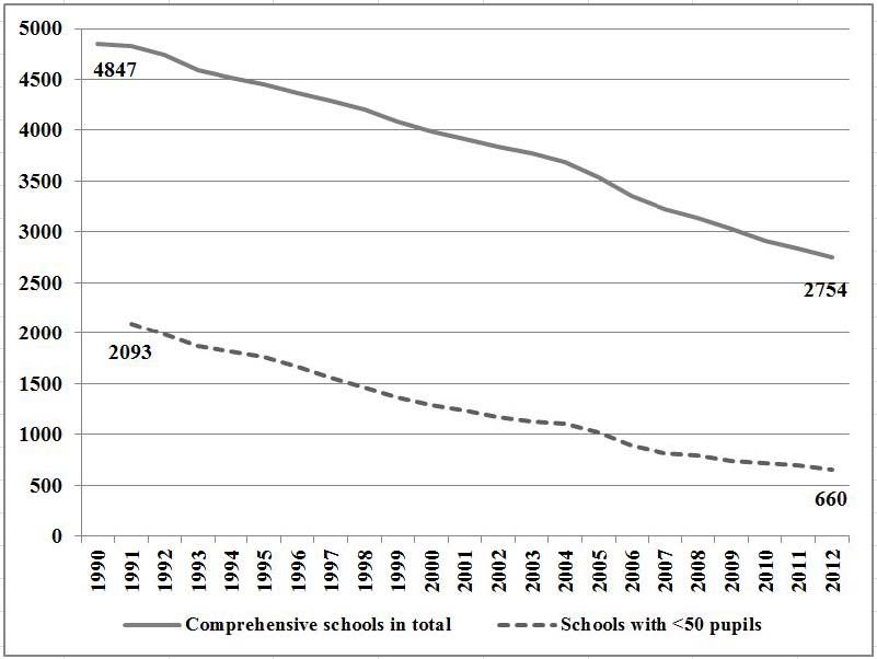
these closures have fallen on small, often rural, schools of less than 50 pupils. Figure
1 displays the trend in school closures in Finland starting from 1990. The number
of schools has dropped to about 60% of what it was in the beginning of the period.
Likewise, only 35% of small schools remain. The increasing rate of school closures is
mainly attributable to the diminishing size of the age groups and to municipalities’
efforts to cut costs (Autti and Hyry-Beihammer, 2014). This tendency has been
very controversial and strongly opposed by communities (Tokola and Tokola, 2010).
Recently, this controversy has given rise to many objections and raised questions
about the influence of school closures on local communities. Among the concerns
aired in the media and in public debate is that the quality of education drops for the
displaced students and that they may suffer negative effects on achievement (Pönti-
nen, 2015a). Policymakers are criticized for ignoring the impact of displacement
on children and are urged to heed this concern in their decision-making (Pöntinen,
2015b).1 Given these concerns, understanding how school closures affect student
achievement is essential for policymakers.
The claims of adverse effects have not been substantiated with evidence nor have
clear channels been proposed through which the possible effects might operate. Sev-
eral mechanisms can be hypothesized: on one hand, displacement may increase the
duration of journeys to school, causing strain on students who have to spend more
time daily on traveling; changes in peer networks and friends may cause disruption
that is reflected in grades; larger class sizes in the receiving school may also have
adverse effects on performance. On the other hand, changing to a bigger school may
1
(Tokola and Tokola, 2010), (Pöntinen, 2015a) and (Pöntinen, 2015b) are articles in a popular
Finnish news magazine, Suomen Kuvalehti.1 Introduction 2 Figure 1: Comprehensive schools in Finland from 1990 to 2012. Source: Autti and Hyry-Beihammer (2014). also have positive influences; the potential size of social networks is bigger in larger schools; moving to a single-age classroom may have an advantage over multi-age classrooms in very small schools; the teachers and curricula could be better in larger schools. The aggregate impact of these factors is ambiguous and an open empirical question which this paper sets out to study. This paper combines several nationwide data sets to identify displaced students in the years 1999-2000 and to study the effects of displacement on medium-term achievement outcomes, such as grade point average (GPA) and the probability of graduating from high school. The sample of students in this study are displaced ei- ther at the end of the fourth or fifth grade. The outcomes are measured four or five years later at the end of compulsory education. Graduation is observed after high school. Because school closure is not random, displaced students may differ system- atically from their peers in factors that correlate with achievement. For example,
1 Introduction                                                                                3

compared to their peers, displaced students generally come from smaller schools in
lower-income rural areas: these are factors that may well influence achievement. To
address this problem, displaced students are matched to comparable students from
a control group. Because cost savings are used as the sole justification for closing
small rural schools with few students, school size and grade size2 are considered to be
the most important controlling covariates used in the matching. A genetic matching
algorithm developed by Diamond and Sekhon (2013) is used to achieve maximum
covariate balance between the treatment and control groups, which is essential for
the credibility of the matching identification strategy.

I find no negative impacts from displacement in any of the measured outcomes.
Displaced students fare no worse than their peers in the matched sample in terms
of school grades, high school graduation rates and high school admission rates.
However, the confidence intervals are relatively large, and small effects on these
outcomes may go undetected. The results indicate that adverse effects on students’
school performance does not have empirical support as an objection to the school
closure policies. However, this study only examines one facet of the many claims
of the negative effects of school closures. It does not evaluate the impact of school
closures on local communities in any broader sense.

The paper proceeds as follows: Section 2 reviews the relevant literature on the effects
of school closings. Section 3 describes the data in detail, and how it is processed.
Section 4 introduces the causal inference framework and delineates the theory of
the matching procedure. Section 5 describes the specification used in the matching,
assesses covariate balance and presents the empirical results. Section 6 concludes.

   2
    For example, the grade size of the 6th grade is the number of 6th graders in the school. One
grade can be spread to several classes. Conversely several grades can be in one class in smaller
schools.
2 Literature review 4 2 Literature review The quantitative literature on school closures is still relatively scarce and restricted to very recent publications, while related subjects have a more established body of literature. For example, studies on the voluntary mobility of students consistently point to the adverse effects of mobility on student outcomes (Hanushek et al., 2004; Xu et al., 2009; Booker et al., 2007). Hanushek et al. (2004) found that high stu- dent turnover during the school year was especially harmful. The literature directly addressing school closures is recent and less unanimous. Among the few relevant studies on forced displacement, Sacerdote (2012) examines the effects of Hurricanes Katrina and Rita on evacuees’ academic performance. He finds that evacuees ex- perience significant temporary drops in their test scores in the year immediately following the hurricanes, but quickly recover, and even see gains in their test scores afterwards. The author hypothesizes that the temporary drops caused by disrup- tion are quickly offset by the higher quality of the evacuees’ new schools. Sacerdote (2012), however, does not study the effect of schools closures, but rather the effect of hurricanes, which come with a plethora of other changes to the lives of the evacuees besides forced displacement. De la Torre and Gwynne (2009) investigate the closure of low-performing schools in Chicago and find that displaced students experience transitory drops in their test scores. Additionally, the authors discover that students who were transferred to higher-quality schools made permanent gains in learning. They use propensity score matching to find schools that are comparable in their characteristics to the closed schools and then use difference-in-differences analysis within the matched sample to arrive at the causal estimates of displacement. A comprehensive study by Engberg et al. (2012) evaluates the effect of the closure of approximately 20 schools in an urban setting. The authors use school assignment, based on catchment areas and students’ addresses, as an instrument for school choice to address non-random sort- ing of students into schools after displacement. They find that displacement has a
2 Literature review                                                                 5

persistent, negative effect on achievement, but this effect can be substantially alle-
viated by placing students in higher-performing schools. Engberg et al. (2012) find
no adverse spillover effects on students in schools that receive displaced students.
These results are somewhat contrary to the findings of Brummet (2014), who exam-
ines a large number of school closings in Michigan over the past decade. The author
uses a difference-in-differences approach to take into account the varying achieve-
ment trajectories of students prior to the school closure. He finds that displaced
students are falling behind in their mathematics score already in the year preceding
the closure. They continue to perform poorly relative to their peers the year after,
but recover fully in two or three years. He also finds that the effect of displacement
depends on the quality of the closed school. Students from low-performing schools
perform relatively better after displacement compared to displaced students from
better-performing schools. The author also finds modest negative spillover effects on
students in receiving schools that depend positively on the quality of the displaced
students.

Overall, existing literature seems to suggest that forced displacement of students
has no persistent negative effects on test scores. Students may experience small,
transitory shocks due to the disruption, but in the long run fare no worse than their
peers. The variation in the results of different studies likely pertain to differences
in specific school closure policies. “School closure” effectively becomes a different
treatment that depends on the particular ways students are redistributed to new
schools etc. The current study seeks to contribute to the existing literature in two
ways. First, the study examines school closure policies that are mainly motivated by
cost savings and not school performance, which is unobserved by the authorities.3
Second, the closed schools that are analyzed are in rural areas where distances are
long and class sizes very small. Displaced students move to bigger schools, with

  3
      There are no nationwide standardized tests for primary schools in Finland.
3 Data 6
larger class sizes. The treatment, therefore, includes the change in distance and
class size as well as disruption and other factors present in the settings of other
studies. Increased class size after displacement could be expected to have a lasting
negative impact on achievement (Krueger, 1997; Krueger and Whitmore, 2001),
although it is not clear how class size dynamics affect achievement in very small
class sizes. Increased school distance is also hypothesized to have a negative effect
on student outcomes. Longer distances mean longer school trips and less free time,
with potential ramifications for academic performance.
3 Data
The objective of this study is to identify the effect of displacement on student
achievement as measured by grades, secondary education admission rates and high
school graduation rates. More specifically, due to data restrictions, the treatment
for any student is defined as being displaced due to school closure during the last
two years of primary school.4 Unlike voluntary mobility, school closures always take
place at the end of the school year, in spring. Therefore, displacement means that
the student starts his next school year at a different school. The outcomes are mea-
sured four or five years later in the joint application system at the end of ninth
grade. This is the first time grades are recorded in a national database and can be
compared. Records of earlier grades are not available for any student, otherwise the
identification of this study could be improved to take into account the trajectories
of the outcome variables. High school graduation rates are observed ex post facto.
Compulsory education in Finland lasts for nine years or until the student is 17 years
of age. Primary schools comprise grades 1-6 and lower secondary schools comprise
4
At the end of the fourth or fifth grade.3.1 Joint application data 7 grades 7-9. Comprehensive schools offer all grades from 1-9, i.e. they include pri- mary and lower secondary schools. However, particularly in rural areas, there are many primary schools offering various combinations of grades, for example only grades 1-2, and students may attend several schools during their primary educa- tion. Comprehensive schools in the countryside are also very rare. All the displaced students in this study attended primary schools and went to a different school for grades 7-9. This means that displacement affected them only for one or two years. 3.1 Joint application data This study uses the data collected by the joint application system as the primary source of student-specific variables. The joint application system is a nationwide application process which is the only channel for applying to upper secondary edu- cation after completing compulsory education. The dataset is collected biannually and includes all individuals in two categories in the Finnish school system. The first category comprises individuals who are in the ninth, and usually last, grade of the compulsory education system. These are automatically registered in the joint application system (even if they do not apply to any school). The second category is individuals of different ages who, for whatever reason, apply for upper secondary education. These two categories usually overlap significantly, as most applicants for upper secondary education are those who are just about to finish compulsory education. The dataset is maintained by the Finnish National Board of Education. It is non- public and access to it was obtained for this study through the VATT Institute for Economic Research. Reproduction of the results of this paper will require access to this dataset. The dataset used in the current study spans from 1997 to 2004. Earlier years are not available and later years do not include address data for individuals, which are crucial for sorting individuals to schools. The raw dataset has 771,447 entries where the unit of observation is an applicant in a particular year. Even
3.1 Joint application data                                                                       8

though this is not panel data, students can occasionally appear in the data multiple
times. This is either because they have applied multiple times, or because they first
applied after ninth grade, but were also automatically registered at ninth grade.

This study excludes all observations not reported to be in the ninth grade, which
ensures that only the first entry of any individual is taken into account. This en-
try will reveal all relevant information about the individual, including grades and
whether she actually applied or not. After this exclusion 513,191 entries remain.

A key to determining the treatment status of students is knowing which primary
school(s) they have attended. This information is missing from the joint applica-
tion data and is not readily available anywhere. For the purpose of the present
study, this becomes an estimation problem of sorting students to primary schools.
It is an especially challenging problem for a number of reasons. Firstly, the par-
ticular catchment area of each school is obscure, which complicates address-based
sorting. Secondly, the computational demands are potentially overwhelming when
students are sorted based on distances to schools (the approach adopted in this
paper). Thirdly, small mistakes in school locations and student sorting can lead to
large errors in the determination of the treatment status. The remaining paragraphs
of this Section describe my attempt to address each of these challenges.

In each grade, students are assumed to attend the nearest school which offers that
grade (not all primary schools offer all grades). Address information from the joint
application is used as a proxy of students’ addresses in the last two years of primary
school.5 There are two obvious caveats that would introduce error into the sorting
of students to primary schools: (1) students may attend a school other than the
nearest one; (2) the address used as a proxy is different than the actual address at

   5
    Address history is available from Statistics Finland for a price, which was beyond this project
for both time and financial reasons.
3.1 Joint application data 9
the end of primary school, i.e. the student has moved between the end of primary
school and ninth grade.
The focus of this study is on small schools in scarcely populated areas. Even though
the legislation in Finland changed in the 1990s to permit students to attend schools
outside their catchment area, this legislation was only gradually adopted by mu-
nicipalities and, in practice affects less residents of rural areas, who still typically
attend their nearest school (Seppänen, 2006). The latter caveat remains a problem.
However, migration of families with children from rural areas is low (Table 1, page
27) and I will have to accept the measurement error it introduces.
Some students attend private schools, such as Rudolf Steiner schools, various lan-
guage schools, or special education schools.6 The primary mechanism for selection
to these schools is not proximity. Such students are therefore excluded from the
analysis, reducing the number of observations to 498,329.
Student addresses are converted to map coordinates using the geocoding software
ArcGIS and cross-validating the results with the online geocoding service GPS Vi-
sualizer. Imprecise coordinates can mostly be attributed to typing errors in the
addresses, and similar random mistakes. Excluding these takes the number of ob-
servations to 480,701, representing an accuracy of about 96.4% (exact matches).
The remaining 3.6% are typically within a few hundred meters of the true location.
6
Almost all special schools are combined primary and lower secondary schools (comprehensive
schools). The latter of these is observed for each student, which is why the primary school of these
students is also known.3.2 Combining the joint application data with school data 10
3.2 Combining the joint application data with school data
School-level variables are taken from panel data compiled in VATT using data ob-
tained from Statistics Finland. The data covers the years 1998-2003 for each school
and includes variables such as cohort7 size for each grade, the number of enrolled
students in the fall/spring, and a dummy for closure. The overlap between the two
datasets is three years 1998-2000 in the schools data, corresponding to 2002-2004
in the joint application data. The ninth graders registered in the joint application
data in 2004 graduated from fifth grade in 2000. Therefore, 2000 is the last year
when they could be displaced, in which case they would start their final year (fall
2000) of primary education in a different school. Equivalently, the ninth graders of
2002 are the last cohort to attend primary schools in 1998.
Cohort size per grade level is an important control covariate in this study. It natu-
rally has a value of zero for the year a school was closed.8 A straightforward way to
approximate the “potential” cohort sizes9 for that year is to extrapolate the values
of the previous year. This is the approach followed in this study. Schools that were
closed in 1998 have no previous values to extrapolate from and must be excluded
from the analysis. Two years of cohorts remain after these considerations: 1999-
2000 from the school data corresponding to 2003-2004 in the joint application data.
This brings the number of observations down to 118,332.
In total these two years have three distinct cohorts of displaced students:
1. Students who were in the ninth grade in 2004 and were displaced in 2000 after
grade five.
7
From hereafter, cohort signifies students of a particular grade in a particular year (for example
sixth graders in 1999).
8
Cohort sizes are registered in the fall.
9
The cohort sizes the school would have had if it had not been closed down.3.2 Combining the joint application data with school data 11
2. Students who were in the ninth grade in 2004 and were displaced in 1999 after
grade four.
3. Students who were in the ninth grade in 2003 and were displaced in 1999 after
grade five.
School addresses are taken from the 1997 paper edition of the School Catalogue
published by Statistics Finland, and are combined with the school data by school
code (a unique identifier for every school). A geocoding process similar to that
used for student addresses was employed to transform the school addresses to map
coordinates. However, many schools, especially in more peripheral areas, either do
not have an address or only report a postal box number. Errors in school coordinates
potentially lead to large errors in determining the treatment status of students in the
data. For example, misplacing a small closed school in a more densely populated area
not only wrongly sorts a large number of students from that area to the treatment
group, but also sorts the students who are actually displaced to the control group.
Omitting a school from the data also sorts its students erroneously. For this reason,
extensive efforts were made to find the actual geographical location of each and
every school in the data (3078 schools). This involved calls to municipalities and
local residents and in some cases much use of map services, image search, and Google
Street View. Due to these extensive measures, the accuracy of the school coordinates
is close to 100%. All special schools are removed from the school data to match the
corresponding removal of special school students from the joint application data.
Each student is sorted to a school separately for grades five and six so that the
distance from the coordinates of her proxy address to the coordinates of the school
is minimized within the set of all schools. Additionally, each student is given a
second-closest school for both grades, which is the school the student would attend
if her school was closed and she was displaced. The R code was optimized to3.2 Combining the joint application data with school data 12
Grade size estimation error for the displaced
60
50
40
Frequency
30
20
10
0
−25 −20 −15 −10 −5 0 5 10
estimated grade size − true grade size
Figure 2: Histogram of grade size error produced by the “nearest school” sorting al-
gorithm. The plotted variable is the difference between the estimated grade size of a
particular closed school in the year of closure and the known (extrapolated) grade size
in the same year. The grades of all three cohorts of displaced students are included.
The number of observations is 201 grades corresponding to 775 actual students and 867
estimated students.
complete its run overnight.10
Figure 2 shows how accurately the displaced students where sorted to their schools.
I am satisfied that the mode of the estimation error is zero and, with the exception
of one outlier, serious underestimation of size concerns relatively few grades. On the
other hand, there are more grades to which excess students have been sorted. These
estimation errors could be explained by some students having better connection to
10
The R software environment was used for both data management and empirical analysis.3.2 Combining the joint application data with school data 13
Grade size estimation error for the displaced
120
100
80
Frequency
60
40
20
0
−25 −20 −15 −10 −5 0 5 10
estimated grade size − true grade size
Figure 3: Histogram of grade size error after removing excess students from each grade.
The errors in grades to the right of zero in Figure 2 are forced to zero. The number
of observations is 201 grades, corresponding to 775 actual students and 593 estimated
students.
a school other than the nearest one due to geographical (rivers) or infrastructure
barriers (bad roads), which are not captured by straight-line distance. This is then
reflected in the catchment areas set by municipal authorities. It is reasonable to
assume that grades whose size was underestimated do not contain students who
were erroneously sorted, but rather are missing some students who should have been
sorted there. The contrary must be true for overestimated grades. The number of
students in excess of the known grade size cannot have attended the school. Some
students would then have been erroneously sorted to the treatment group (displaced
students), which would bias any treatment effect estimates. I propose a simple
solution, which is followed in this study: For each grade, the students living further
away from the school are more likely to have been sorted incorrectly compared to4 Methods 14 students nearer to the school. Take X number of the furthest-away students in each grade and omit them from the data, where X is the number of excess students in that grade. After this exclusion, 99,161 observations remain. Figure 3 shows that this operation has forced to zero the estimation errors of previously overestimated grade sizes. For the purpose of this study, students at schools that are consolidated instead of closed are treated as if their school never closed. Consolidated primary schools are identified by the fact that they share an address with a lower secondary school which starts to offer primary school grades in the same year as the primary school closes. The new school becomes a comprehensive school. No observations are lost in this reclassification of treatment status. However, it happens that during the period studied here, consolidations take place almost exclusively in cities, whereas closures only occur outside cities in small schools of less than 90 students. Therefore, this reclassification effectively changes the focus of this study to scarcely populated areas. 4 Methods Causality can have many connotations and interpretations in different contexts. In the context of this study, and in applied microeconomics more generally, causality is a comparison between the observed world and a counterfactual, hypothetical re- ality where the cause (e.g. displacement) is not present. The effect of a cause on some variable is the difference between the values of that variable in the observed world and its values in the counterfactual world where that cause did not occur. It answers the question “what would have happened to the student if she had not been displaced?”. The true causal effect is always theoretical and unobservable, since we can never experience the counterfactual world where the cause was not present. Therefore, determining the causal effect becomes an estimation problem which this
4.1 Potential outcome framework 15
section attempts to address in the context of the present study.
4.1 Potential outcome framework
The potential outcome framework developed by Rubin (1974, 1978) is widely used
for identifying causal effects in observational studies. The following is a brief re-
capitulation of its fundamentals for the purpose of this study. I follow the more
recent notation of Angrist and Pischke (2008) for clarity of exposition. The current
study warrants the use of a causal model because it is interested in the causal effect
of school closures on student achievement. The simple difference in the means of
the grade point averages at the end of the ninth grade between students who were
displaced by a primary school closure and those who were not is about -0.1 grade
points. Therefore, on average, non-displaced students perform better than displaced
students. This relationship, however, is not necessarily causal as there are many po-
tential ways for the two groups to differ in factors that influence students’ grade
point average. For example, most displaced students attend small rural schools,
which may provide inferior education or have more stringent grading. Or perhaps
they come from less educated family backgrounds, or from low-income districts,
which are well documented to correlate with academic performance (Sirin, 2005).
Formalizing the problem, let displacement for student i be described by a binary
variable Di = {0, 1}. The observed outcome of interest, student achievement, is de-
noted by Yi . The question is how much Yi is affected by displacement. The potential
outcomes, Y1i and Y0i , are the values Yi would take in a hypothesized world where
the individual was displaced or was not displaced, i.e. in the presence of treatment
and in the absence of treatment respectively. In the case of a binary treatment, such
as displacement by school closure, each individual has two potential outcomes, only
one of which can be observed as the realized outcome:
Y if D = 1
1i i
P otential outcome = Yi = = Y0i + (Y1i − Y0i )Di (1)
Y0i if Di = 04.1 Potential outcome framework 16
The last term is very informative because Y1i −Y0i is the causal effect of displacement
for an individual student. For every individual, we can only ever observe the one
potential outcome that actually occurred. That is why in this framework we can
never learn about the causal effects of a treatment on an individual level. Meaningful
comparisons can only be made between the averages of those who were treated
and those who were not. The comparison of average outcomes conditional on the
treatment status is linked to the average causal effect through the following equation:
E[Yi |Di = 1] − E[Yi |Di = 0] = E[Y |D = 1] − E[Y0i |Di = 1] (2)
| {z } | 1i i {z }
Observed difference in GPA Average treatment effect on the treated (ATT)
+ E[Y0i |Di = 1] − E[Y0i |Di = 0]
| {z }
Selection bias
The observed difference in average GPA can be expressed in two terms by adding
and subtracting E[Y0i |Di = 1]. The average treatment effect on the treated (ATT) is
the average causal effect of displacement in the group of students who were actually
observed to have been displaced. It represents the difference between the observed
GPA of the displaced students and what would have been their GPA had they not
been displaced. This is the quantity we are interested in estimating. However, the
observed difference in average GPA also includes a selection bias term, which is the
difference in average Y0i between the treatment and control groups. In the current
study an example of negative selection bias is that displaced students would have
lower GPAs even if their school had not closed. Selection bias accounts for the entire
observed difference in means when the treatment effect is zero. To identify the true
ATT, this problem needs to be addressed.
The selection bias term in the equation disappears and the selection problem is
solved when Di is independent of potential outcomes. The observed difference in
GPA becomes precisely the ATT. To see this, notice that because of the indepen-
dence of Di and Yi , we can substitute E[Y0i ] = E[Y0i |Di = 1] for any term on the4.1 Potential outcome framework 17
right-hand side of equation (2), thus making the selection bias term disappear.11
Random assignment of the treatment is a straightforward way to achieve this in-
dependence, which is why randomized controlled trials (RCT) are considered to be
the benchmark in causal inference. In the current observational study, random as-
signment of the treatment is of course impossible because the data has already been
collected. Nevertheless, a useful mental exercise at this juncture is to imagine an
ideal experiment that we would like to set up to identify the causal effect, if we
had unlimited resources and didn’t care about ethical issues. A plausible scenario
would be to randomly assign elementary schools to treatment and control groups,
and then close down the schools in the treatment group and compare the outcomes
in the ninth grade. This exercise shows that the question this study tries to address
is a valid causal question that could be answered with an RCT.
Finally, causal inference is not valid unless “the (potential outcome) observation
on one unit should be unaffected by the particular assignment of treatments to the
other units” (Rubin, 1978). Having developed the potential outcome framework, let
us apply it to formalize this Stable Unit Treatment Value Assumption (SUTVA):
T
YitTi = Yit j ∀ j 6= i, (3)
where Ti is the treatment assignment for unit i, Tj denotes the treatment assign-
ment for unit j, and t ∈ 0, 1 represents the potential outcomes under treatment and
control. SUTVA implies that the potential outcomes of student i, Yi1 and Yi0 , do
not in any way depend on the treatment status of any other student in the dataset.
Violations of SUTVA pose a threat to valid inference, because the comparison is no
longer between the group that is influenced by the treatment and the group that is
not. Rather, some individuals in the control group are also affected by the treat-
11
By the same token, the ATT could further be reduced to just the average effect of displacement,
E[Y1i − Y0i ].4.2 Matching identification 18 ment, thus biasing the estimates. For example, displaced students might influence the academic performance of their peers in the receiving schools. Through this dy- namic, displacement not only influences the outcomes of the displaced, but also the outcomes of students in the control group. Therefore comparing the outcomes of these individuals is meaningless, because the affected non-displaced students are no longer a credible counterfactual. To address potential SUTVA violations, students at primary schools that received displaced students (second-nearest school for dis- placed students) and students who shared lower secondary schools with displaced students are removed from the data. This should eliminate any immediate SUTVA violations from the analysis. Additionally, it removes displaced students who are falsely sorted to the control group because they attended their second nearest school, which was shut down, instead of their nearest school. Ultimately, this makes the total number of observations 81,135, of which 596 are displaced. 4.2 Matching identification In observational studies there are multiple “identification strategies”, ways of at- tempting to solve the selection problem, most typical of which are instrumental variable estimation, difference-in-differences estimation and fixed effect estimation (Angrist and Pischke, 2008). Finding the most suitable strategy is situational and depends on the particular setting at hand. The joint application data that is used in this study restricts the number of viable identification strategies because it is not panel data: each student is observed only once, at the end of their compulsory education. This makes student-level difference-in-differences, such as those used by De la Torre and Gwynne (2009) and Brummet (2014), and some fixed effect strategies unviable. Difference-in-difference estimation is based on projecting the counterfactual trajectory of the outcome variable in the treatment group using the trajectory of a comparable control group that was not treated. The causal effect is the size of the treatment group’s observed deviation from this projection. Multi-
4.2 Matching identification                                                         19

ple observations of the outcome variables are necessary for the employment of this
strategy, which makes it impractical for the setting of this study. Using instrumental
variables estimation depends on having high-quality instruments for school closing,
which are hard to find or non-existent. A valid instrument would have to influence
the achievement outcomes through school closures alone. Unlike for Engberg et al.
(2012), neither the catchment areas of schools nor school choices are observable in
the current setting, which is why school assignment cannot be used as an instrument
for school choice as the authors do. Matching suits the current setting particularly
well for two reasons: It mimics the ideal experiment that was laid out in the last
chapter, and it does not require panel data. The genetic matching algorithm that
is used for matching is also non-parametric and does not make any distributional
assumptions, which is a clear advantage over parametric methods.

It is impossible to calculate the ATT in equation (2) directly because Y0i is not
observed for the treated. This problem can be overcome by assuming that treatment
assignment depends only on the observable covariates X. Following Rosenbaum and
Rubin (1983), treatment assignment is said to be strongly ignorable if it satisfies the
following conditions for every i:

                                    {Y0 , Y1 } ⊥⊥ Di   |X                          (4)
                                0 < P (Di = 1|X) < 1

The first condition expresses the conditional unconfoundedness of the treatment
assignment: the distribution of potential outcomes are the same in the treatment
and control groups conditional on the covariate vector X. Confounders are variables
that influence the outcomes, but they are not necessarily equally distributed between
the groups. All confounders must be included in X for conditional unconfoundedness
to hold. This conditional independence is precisely what is required for the selection
bias to disappear in equation (2). The second condition expresses common overlap
of covariates between the two groups. In order for matching methods to identify
4.2.1 Balancing score and the propensity score 20
the causal effect, the control group must have at least one individual with similar
covariate values to the treatment group, or vice versa. For estimating the ATT
these condtions can be relaxed to Y0 ⊥⊥ Di | X and P (Di = 1|X) < 1. Under these
assumptions the ATT in equation (2) can be expressed as follows:
AT T = E{E[Y1i |Di = 1, Xi ] − E[Y0i |Di = 0, Xi ]|Di = 1} (5)
Where the outer expectation is taken over the distribution of X in the treated
group, Xi |(Di = 1) (Sekhon et al., 2009). Finally, all the variables in equation (5)
are observble and the ATT can be estimated.
4.2.1 Balancing score and the propensity score
In the estimation of the ATT, the most obvious way to condition on X is to find in
the control group exact matches for each unit in the treated group. This is, however,
unviable when the vector of covariates, X, is long or there are continuous variables
and common overlap is not perfect. A balancing score can solve this problem. The
balancing score, b(X), is a function of the covariate vector X, so that conditional
on b(X), the distributions of the covariates in the treatment and control groups are
in balance, X ⊥⊥ Di | b(X). Rosenbaum and Rubin (1983) show that if treatment
assignment is ignorable conditional on X, then it is also ignorable conditional on any
balancing score b(X), and this balancing score can be used in equation (5) instead
of X.
Which balancing score should be used? A widely used method is to estimate the
propensity score; the probability of being treated conditional on the observed co-
variates P [Di = 1|X] (Diamond and Sekhon, 2013). The idea of the propensity
score is to match individuals who, based on the observed covariates, are equally
likely to belong to the treatment group. This emulates the randomness of treatment
assignment in an RCT. Given that there are no unobservable confounders, the only4.2.2 Genetic matching 21 difference between these matched individuals is the as-good-as-random treatment assignment. A difference in the means of the outcome would then provide an unbi- ased estimate of the ATT. Rosenbaum and Rubin (1983) prove that the propensity score is a balancing score, and matching on the true propensity score would therefore result in (asymptotic) covariate balance between the treatment and control groups. Conversely, the estimated propensity score is consistent only if the observed con- founders are balanced after matching. This tautology can be used to assess the quality of an estimated propensity score by looking at the covariate balance in the matched sample (Diamond and Sekhon, 2013). Since the functional form of the true propensity score is generally unknown, a logit regression is usually estimated on the covariates to obtain a scalar quantity (the estimated propensity score), which is then used to find the nearest matches in the control group. Assessing covariate balance after matching and then adjusting the logit model to improve balance are important parts of this matching method (Diamond and Sekhon, 2013). However, finding the propensity score that achieves balance on a large number of covariates is not a trivial problem, and quickly becomes a laborious guessing game. Possible specifications of the propensity score, with interaction and square terms, are numerous. Moreover, tinkering with the specification after each iteration does not guarantee improvement of the overall covariate balance. 4.2.2 Genetic matching Diamond and Sekhon (2013) propose a genetic search algorithm (GenMatch) to address the problem of finding a balancing score that optimizes the post-matching covariate balance. GenMatch uses a scalar quantity distance metric to measure the multivariate distance between the covariates of two individuals. The Generalized
4.2.2 Genetic matching                                                                     22

Mahalanobis Distance12 between the the X covariates of two individuals i and j is

                                q
            GM D(Xi , Xj , W ) = (Xi − Xj )T (S −1/2 )T W S −1/2 (Xi − Xj ),              (6)

where W is a kxk positive definite diagonal weight matrix, S is the sample covariance
matrix of X and S −1/2 is the Cholesky decomposition of S, i.e. S = S −1/2 (S −1/2 )T .
The sample covariate matrix X may contain terms that are functions of X, including
the propensity score itself. The GenMatch algorithm searches for weights W that
optimize the post-matching covariate balance. Each potential value of the distance
metric corresponds to a particular assignment of weights. Given the weight matrix,
matching (for the ATT) is done for each unit in the treated group by finding a unit
in the control group that minimizes the distance as measured by equation (6).

The algorithm automates the iterative process of testing post-match balance, and
adjusting the proposed distance metric to improve the balance. The measure of
balance is specified by the user in the loss function. GenMatch chooses weights,
W , that minimize this function (maximize balance). The loss function used in the
present study is specified in the following section.

GenMatch uses an evolutionary search algorithm to choose the weights that optimize
the specified loss function. The algorithm starts with a batch of initial weights, W s.
Each batch is a generation that is used iteratively to produce the next generation of
weights with balance-improving values. The population size of each generation can
be specified by the user and is constant throughout generations. Larger population
sizes generally achieve better overall balance. Figure 4 summarizes the algorithm.
Notice that the outcome variable is not used at all during the process. GenMatch

  12
   This is the authors’ generalization of the familiar Mahalanobis Distance, which is used for
matching in statistics.
4.2.2 Genetic matching 23
Figure 4: Flowchart of the Genetic Matching Algorithm. Source: Diamond and Sekhon
(2013)
simply modifies the distance metric until the optimal post-matching covariate bal-
ance is achieved.
Diamond and Sekhon (2013) summarize the iterative process as follows:
“For each generation, the sample is matched according to each metric,
producing as many matched samples as the population size. The loss
function is evaluated for each matched sample, and the algorithm iden-
tifies the weights corresponding to the minimum loss. The generation of
candidate trials evolves toward those containing, on average, better W s
and asymptotically converges toward the optimal solution: the one that
minimizes the loss function.”5 Empirical analysis 24 5 Empirical analysis 5.1 Covariate balance In a matching identification strategy such as this, valid causal inference depends on whether the ignorability conditions (4) hold. The extent of common overlap between the treatment and control groups is revealed in the degree of covariate balance achieved after matching. A perfect balance implies perfect overlap and overall imbalance implies that the algorithm couldn’t find close matches. In the current study, the quality of matches, and therefore common overlap, proves to be high in the chosen covariates. This is due to the large variability, relative to the treated group, in the covariate values of the control pool of potential matches. The conditional unconfoundedness, a.k.a. selection on observables, assumption states that we observe all covariates that correlate with the selection to the treatment group as well as with the outcome. Conditioning, i.e. matching, on these covariates makes the treatment assignment as-good-as-random between the groups in the sense that the potential outcomes are equally distributed between them. However, there is no way of testing this assumption empirically. Some credibility could be given to it by conducting placebo tests on pre-treatment outcome variables. Placebo tests are balance tests applied to outcome variables of the matched sample before treatment takes place. Before the treatment, Y0 is observed for both groups. If the selection on observables assumption holds, the distribution of Y0 should be equal in both groups. Observing otherwise would undermine the plausibility of the assumption. In this study, this would amount to testing whether the displaced and non-displaced groups in the matched sample have similar distributions of grades, say, in the fourth grade. Conducting placebo tests requires pre-treatment observations of the outcome vari- ables. These are not available to me, since grades are recorded in the system only at the end of the ninth grade. Evidence beyond the statistical methods must therefore
5.1 Covariate balance                                                                             25

                               Balance Before Matching                 ●   t−test
                                                                           Equivalence test
                    Variable   Treatment   Control−pool
                      Name         Mean           Mean

                       Male        0.54          0.507            ●

            Finnish speaker       0.985          0.918    ●

              Finnish school      0.992          0.961    ●

                 Grade size          4.8          44.7    ●

                 School size       25.1          261.9    ●

          Distance to school       2.44           1.13    ●

      School size 2nd school         98          220.2    ●

      Distance to 2nd school         5.7          2.87    ●

             Primary school       0.995          0.902    ●

                       Year      1998.6         1998.5        ●

                                                          0 .05 .1                            1
                          N         596          80539
                                                                      p−value

Figure 5: Pre-matching balance plot displaying the covariate balance between the treat-
ment group and the control pool for covariates included in the matching. Each covariate
corresponds to the value of the variable when the students were in grade five.

be used to convince the reader of the plausibility of the assumption. My choice of
control covariates is limited to the variables included in the school data or recorded
in the joint application data for each individual. Figure 5 displays the balance plot
summarizing the covariate (im)balance between the groups before matching is con-
ducted. Male and Finnish speaker are taken from the joint application data and the
remaining variables are derived from the school data. The control covariates must
be measured before treatment takes place (or possibly even announced). Otherwise,
the treatment could affect these “bad control” variables biasing the estimates, if
they are used in matching (Angrist and Pischke, 2008). However, there is no reason
to exclude from matching any variables that are fixed and cannot be affected by
displacement. This is why the gender and mother tongue variables can be included
from the joint application data, even when they are collected after displacement.
The pre-treatment data available for this research comes from the school dataset.
5.1 Covariate balance 26
Students are matched based on their fifth-grade values of each covariate. For the
displaced students, School size and Grade size are extrapolations of the respective
values from the end of fourth grade. Distance to school and Distance to 2nd school
are the distances (km) to the nearest school and second-nearest schools that would
offer grade five if the school was not closed down. The nearest school is the school,
that the student would attend if it was not closed, and the second-nearest school
is the school she attends if she is displaced after grade four. Finnish school and
Primary school are additional pre-treatment indicator variables that are controlled
for. Year controls for the age of the students at grade five.
Grade five is used as the covariate baseline for a practical reason, simply because
it is the latest grade which is pre-treatment for all observations. If grade six was
included, some of the students would already have been displaced and the variables
would represent values for the school that received the students, values which are
determined by the treatment. The p-values of the t-tests and equivalence tests
are shown on the right-hand side.13 The imbalance between the treatment and
control groups is clear. Almost all the covariates are significantly different between
the groups. The school sizes and grade sizes are roughly ten times bigger in the
control group. The distances to school are also twice as long in the treatment group
compared to the control group. These differences arise from the rural location of the
closed schools. The population densities are much smaller and the school network
is sparser, which results in smaller schools that are far apart from each other.
Another potential source of covariates is the zip code-specific database maintained by
Statistics Finland. However, for this study, the earliest available year of zip code data
is 2001, which is just the year after the last cohort of students was displaced. These
13
The equivalence test uses two one-sided t-tests to test the null hypothesis of inequality between
the groups. The regular t-test favors the researcher in the null hypothesis of zero difference, which
is why equivalence tests are used to supplement the balance analysis.5.1 Covariate balance 27 Table 1: Descriptive statistics based on zip codes. Comparison before matching. Variable name Treatment Mean Control-pool Mean Swedish speakers, % 0.8 5.4 Average income, ¿/year 13, 984.0 18, 131.0 Median income, ¿/year 11, 207.0 15, 073.0 Average size of school aged households 4.6 4.3 Labour force academic degree, % 7.4 13.7 Labour force vocational degree, % 58.5 55.2 Population density, persons/km2 30.3 829.2 Fraction of out-migrants, % 6.9 10.3 Fraction of in-migrants, % 5.5 10.2 Households with school aged children, % 13.9 14.5 Unemployment rate, % 17.8 13.5 N 596 80, 539 Average size of school aged households is the average size of households that have school aged children. Labour force vocational degree is the fraction of the local labour force that has a secondary education vocational degree (high school level). Labour force academic degree is the fraction of the local labour force that has a higher education degree. Fraction of out-migrants is the fraction of population that have moved out of the area during the last year. Fraction of in-migrants is the fraction of population that have moved into the area during the last year covariates would suffer from the “bad control” problem if matched on, and cannot therefore be used as control covariates. Table 1 presents a selection of covariates that are possible confounders. The table of means is constructed so that every student gets the value that corresponds to the zip code of her address. On average, displaced (treated) students come from poorer, less educated areas that are sparsely populated. These areas have higher unemployment rates, marginally bigger families and lower migration rates. These statistics are consistent with prior knowledge of the location of closed schools in rural areas. Displacement may have little effect on these variables in one or two years due to low mobility and the flat short-term trends of most of these variables. Nevertheless, because of the bad control problem, I am apprehensive of using them in matching.
5.1 Covariate balance                                                                                28

                                  Balance After Matching                  ●   t−test
                                            Matched                           Equivalence test
                     Variable   Treatment
                                             Control
                       Name         Mean
                                              Mean
                        Male       0.541      0.541                                              ●

             Finnish speaker       0.985      0.985                                              ●

               Finnish school      0.992      0.992                                              ●

                  Grade size        4.82       4.84                                       ●

                  School size       25.2       25.6                            ●

           Distance to school       2.44       2.34                   ●

       School size 2nd school       97.9       94.5                                ●

       Distance to 2nd school       5.69       5.87               ●

              Primary school       0.995      0.995                                              ●

                        Year      1998.6     1998.6                                              ●

                                                       0 .05 .1                                  1
                           N         601        601
                                                                      p−value

Figure 6: Post-matching balance plot displaying the covariate balance between the treat-
ment group and the control pool for covariates included in the matching. Each covariate
corresponds to the value of the variable when the students were in grade five.

Several key decisions are required in employing GenMatch.14 The specification in
this study estimates the average treatment effect on the treated (ATT) using one-to-
one matching with replacement, without caliper15 . Estimating the ATT means that
the algorithm searches for matches for the treated units from the control pool, and
not vice versa, which would be estimating the effect on the controls (ATC). Caliber
is not used, because it does affect the outcome of the procedure, since the quality of
matches is high. Binary variables are matched exactly, meaning that the algorithm

  14
     The authors of the GenMatch algorithm have provided a GenMatch package for the R software
environment, which is used in the current paper.
  15
     Caliper is used to discard units for which a match cannot be found that is close enough in
covariate values. Closeness is arbitrarily defined.
5.1 Covariate balance 29
Grade size distributions before matching
Control
Treatment
0.15
0.10
Density
0.05
0.00
0 50 100 150
Grade size at fifth grade
Figure 7: The empirical distributions of grade size in the treatment group and the control
pool.
searches for matches in the subgroup of control units that share the same language,
gender and age as the treated unit. A population size (the size of each generation of
weights) of 5000 is used. A larger population size would make the computing time
prohibitively long. The specification described here produced 28 generations and
took 99 hours to complete its run.
The loss function is specified as a vector of p-values from paired t-tests and Kolmogorov-
Smirnov (KS) tests, which test the equality of each individual covariate within the
matched sample (the vector is twice the length of the covariate vector). The paired
t-test only tests the equality of the means of the covariates between the treatment
and control groups in the paired sample. The KS test, on the other hand, also ac-
counts for the differences in the distributions of covariates between the groups. The
test statistic for the KS test is the longest vertical distance between the two groups’
empirical cumulative distributions of a covariate. GenMatch chooses weights that5.1 Covariate balance 30
Grade size distributions after matching
Control
0.20
Treatment
0.15
Density
0.10
0.05
0.00
0 10 20 30
Grade size at fifth grade
Figure 8: The empirical distributions of Grade size in the treatment group and the
matched control group.
maximize the smallest of these p-values (minimize difference). This loss function
does not give particular significance to the balance of any individual covariate, but
rather maximizes the overall balance. This is an appropriate approach for this study,
because there is no prior knowledge of the importance of any single covariate relative
to others. Additionally, because of the good overlap, there seem to be no notable
balance tradeoffs between the chosen covariates.
Figure 6 displays the covariate balance achieved after matching with the above
specification. As indicated by the p-values, the overall balance is perfect in the
sense that the equivalence tests reject the null hypothesis of difference and the
paired t-tests cannot reject the null hypothesis of equality. The p-values from the
KS-tests are not displayed for visual clarity. They are qualitatively similar to the
p-values of the paired t-tests. The variable Grade size 2nd school is omitted from the
matching procedure because when it was included, the algorithm would not achieveYou can also read