AMICal Sat and ATISE: two space missions for auroral monitoring - Journal of Space ...
←
→
Page content transcription
If your browser does not render page correctly, please read the page content below
J. Space Weather Space Clim. 2018, 8, A44
 M. Barthelemy et al., Published by EDP Sciences 2018
https://doi.org/10.1051/swsc/2018035
                                                                                                                                   Available online at:
                                                                                                                                  www.swsc-journal.org

    TECHNICAL ARTICLE                                                                                                          OPEN          ACCESS

AMICal Sat and ATISE: two space missions for auroral monitoring
Mathieu Barthelemy1,3,*, Vladimir Kalegaev4, Anne Vialatte1, Etienne Le Coarer1,3, Erik Kerstel2,3,
Alexander Basaev7, Guillaume Bourdarot1,3, Melanie Prugniaux3, Thierry Sequies5,3, Etienne Rolland3,
Emmanuelle Aubert3, Vincent Grennerat5,3, Hacheme Ayasso6,3, Arnau Busom Vidal1,3, Fabien Apper8,
Mikhail Stepanov8, Benedicte Escudier8, Laurence Croize9, Frederic Romand9, Sebastien Payan10,
and Mikhail Panasyuk4
1
   Univ. Grenoble Alpes, CNRS, IPAG, 38000 Grenoble, France
2
   Univ. Grenoble Alpes, CNRS, LiPhy, 38000 Grenoble, France
3
   Institute of Engineering, Univ. Grenoble Alpes, Grenoble INP, CSUG, 38000 Grenoble, France
4
   Skobeltsyn Institute of Nuclear Physics, Moscow State University, 119991 Moscow, Russia
5
   Univ. Grenoble Alpes, IUT1, 38000 Grenoble, France
6
   Univ. Grenoble Alpes, Grenoble INP, CNRS, Gipsa-Lab, 38000 Grenoble, France
7
   SMC Technological Centre, Zelenograd, 124498 Moscow, Russian Federation
8
   ISAE-Supaero, Toulouse, 31400 Toulouse, France
9
   ONERA, DOTA, 91120 Palaiseau, France
10
   LATMOS, UPMC, CNRS, 75252 Paris, France

             Received 8 February 2018 / Accepted 14 September 2018

             Abstract – A lack of observable quantities renders it generally difficult to confront models of Space
             Weather with experimental data and drastically reduces the forecast accuracy. This is especially true
             for the region of Earth’s atmosphere between altitudes of 90 km and 300 km, which is practically
             inaccessible, except by means of remote sensing techniques. For this reason auroral emissions are an inter-
             esting proxy for the physical processes taking place in this region. This paper describes two future space
             missions, AMICal Sat and ATISE, that will rely on CubeSats to observe the aurora. These satellites will
             perform measurements of auroral emissions in order to reconstruct the deposition of particle precipitations
             in auroral regions. ATISE is a 12U CubeSat with a spectrometer and imager payloads. The spectrometer is
             built using the micro-Spectrometer-On-a-Chip (lSPOC) technology. It will work in the 370–900 nm
             wavelength range and allow for short exposure times of around 1 s. The spectrometer will have six lines
             of sight. The joint imager is a miniaturized wide-field imager based on the Teledyne-E2V ONYX detector
             in combination with a large aperture objective. Observation will be done at the limb and will enable
             reconstruction of the vertical profile of the auroral emissions. ATISE is planned to be launched in mid
             2021. AMICal Sat is a 2U CubeSat that will embed the imager of ATISE and will observe the aurora both
             in limb and nadir configurations. This imager will enable measuring vertical profiles of the emission when
             observing in a limb configuration similar to that of ATISE. It will map a large part of the night side auroral
             oval with a resolution of the order of a few km. Both the spectrometer and imager will be calibrated with a
             photometric precision better than 10% using the moon as a wide-field, stable and extended source.
             Ground-based demonstrators of both instruments have been tested in 2017 in Norway and Svalbard. Even
             though some issues still need to be solved, the first results are very encouraging for the planned future
             space missions. Data interpretation will be done using the forward Transsolo code, a 1D kinetic code
             solving the Boltzmann equation along a local vertical and enabling simulation of the thermospheric
             and ionospheric emissions using precipitation data as input.

             Keywords: aurora / airglow / spectroscopy / space weather / visible

*
 Corresponding author: mathieu.barthelemy@univ-
grenoble-alpes.fr

    This is an Open Access article distributed under the terms of the Creative Commons Attribution License (http://creativecommons.org/licenses/by/4.0),
                  which permits unrestricted use, distribution, and reproduction in any medium, provided the original work is properly cited.
M. Barthelemy et al.: J. Space Weather Space Clim. 2018, 8, A44

1 Introduction                                                      0experimental imaging techniques is available in Hecht et al.
                                                                    (2006). Strickland et al. (1989), in particular, were able to fit
    Particle precipitations in the upper atmosphere are the main    three parameters (total energetic input, center of the electron
cause of auroral events. They are caused by acceleration            energy distribution, and a scaling factor linked to the atomic
processes in Earth’s magnetosphere, especially in the auroral       oxygen profile) from measurements of three auroral lines.
acceleration zone. These phenomena are the manifestation of         However, from the ground, only a small part of the auroral oval
the magnetosphere-ionosphere coupling between high-latitude         can be seen and reconstruction of larger parts of the ovals is
ionosphere and magnetotail regions (Birn et al., 2012). Each        extremely difficult with these data. Moreover, cloud coverage
of these regions produces different typologies of auroral emis-     prevents a continuous monitoring of the auroral emissions from
sions. Monitoring particle precipitations in the upper atmo-        ground-based stations. In Ny-Ålesund, this cloud coverage can
sphere is an important aspect of space weather studies since        reach 75% on average over a one-year period (Cisek et al.,
these particles can perturb technological systems and infras-       2017). From space, some imagers have been able to take pic-
tructures on Earth and in space (satellites). These particles,      tures of the auroral structure in both limb and nadir configura-
and especially electrons up to 10 keV, deposit their energy         tions. One of the most recent imaging experiments was carried
mainly in the 100–300 km altitude range where auroras occur.        out using the REIMEI satellite (Saito et al., 2011) and espe-
Observational data on auroral emissions at these altitudes can      cially the MAC optical imager was able to perform auroral
give information on particle fluxes at the top of the atmosphere    images (64 · 64 pixels) at 428 558 and 670 nm, at high
which is very important for understanding of space weather          cadency (120 ms). These wavelengths correspond to intense
conditions affecting polar Low Earth Orbits (LEO).                  emissions of respectively molecular nitrogen ions, atomic oxy-
    The altitude range associated with aurora is too high for       gen, and neutral nitrogen. In this respect, it is also important to
balloons, which can reach altitudes up to 50 km, and too low        mention the THEMIS network over Canada, which included
for satellites, which cannot survive for a long period of time      five satellites and a network of ground magnetometers and
at altitudes lower than 300 km. This means that no long-term        20 ground based cameras to reconstruct the precipitation con-
in situ measurements can be made regarding these particle pre-      ditions once every 4 days if weather is clear. Considering the
cipitations. The currently available in situ measurements have      optical part, we propose an architecture with higher time reso-
been obtained using sounding rockets. Almost all other avail-       lution and fewer instruments.
able data were collected by remote sensing of the ionosphere
at these altitudes. Experimental techniques that target optical     2.2 Spectrometers
emissions are particularly powerful since these emissions are
mainly related to the excitation processes associated with               In addition to the intense lines mentioned above, some
suprathermal particles.                                             molecular emissions extend over a broad wavelength range.
                                                                    Very high spectral resolution enables resolving the individual
                                                                    line profiles providing information on the dynamics of the emit-
2 Choice of observable                                              ting species. In the Northern hemisphere, we can mention the
                                                                    Ebert Fastie spectrometers installed at the Kjell Henriksen
    When observing optical emissions several different tech-        Observatory (KHO) near Longyearbyen in the Svalbard archi-
niques may be used. We can distinguish: imagery, spectroscopy,      pelago. Doppler imaging is also able to provide temperature
polarimetry, as well as some combinations of these (such as, for    data (Kaeppler et al., 2015). At lower resolution, vibrational
example, spectropolarimetry).                                       structures of the molecular bands are still accessible and it is
    Polarimetry, especially of the O I red line, has been studied   easier to observe a larger part of the spectra. An example is
since the first measurements performed by Lilensten et al.          the Nigel spectrometer in Antarctica at Dome A (Sims et al.,
(2008). However, in a first stage, our instrumentation will be      2012), which enables retrieving spectra of the aurora from
focused on imagery and spectrometry.                                300 to 850 nm at 1.5 nm resolution; or the auroral spectro-
                                                                    graph of the NIPR (National Institute of Polar Research)
2.1 Images                                                          installed at KHO. A wavelength resolution of 1–2 nm is
                                                                    sufficient to access the vibrational structures of the main
    Imagery of the auroral emissions has been practiced for         molecular bands.
over one century now. The Tromso Geophysical Observatory                 Considering observations from space, we mention the GLO
(TGO) keeps some of the oldest photographic plates (~1910)          experiment that flew in the late 80’s on board of the Space
of auroras taken in Northern Norway (M. G. Johnsen, pers.           Shuttle. Accurate spectra of the airglow have been registered
commun.). In 2017, a large network of all-sky camera surveys        by this instrument (Broadfoot et al., 1997) allowing retrieval
the auroral emissions in black-and-white, in color (Red, Green,     of N2 emissions, but only at the relatively low latitudes visited
Blue) or at some specific wavelength, such as that of spectral      by the space shuttle. If considering auroral regions, the
lines, especially the O I green line at 557 nm, the O I red line    spaceborne spectrometer experiments are mainly dedicated to
at 630 nm or the Nþ   2 band at 427 nm. These ground based          FUV (Far Ultra-Violet) measurements e.g., the UVI (Ultra-Vio-
images give some information on the region of precipitation,        let Imager) on board the Polar satellite (Germany et al., 1998)
on the corresponding magnetospheric L-shell, and on the atmo-       or the TIMED-GUVI (Thermosphere Ionosphere Mesosphere
spheric and magnetospheric dynamics, as well as composition         Energetics and Dynamics)-Global Ultraviolet Imager experi-
changes induced by these precipitations. A review of the            ment (Christensen et al., 2003).

                                                            Page 2 of 12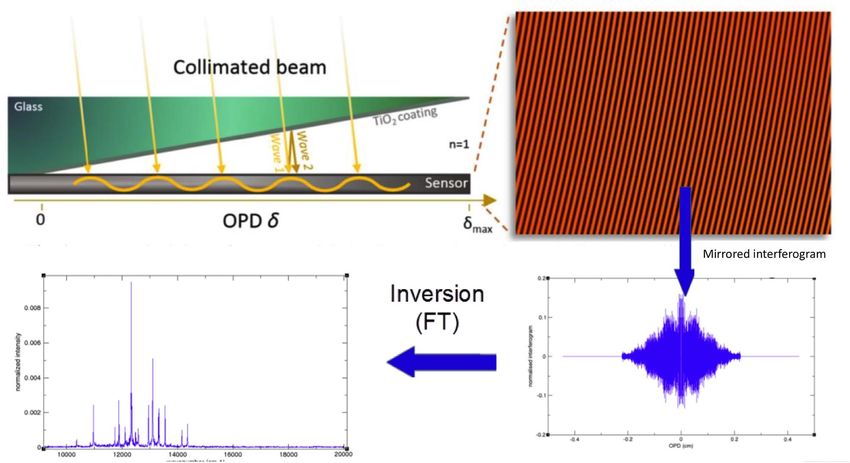
M. Barthelemy et al.: J. Space Weather Space Clim. 2018, 8, A44

Fig. 1. Schematic representation of the SPOC principle.

2.3 Retrieval of the vertical profile of the auroral                 recently by IPAG and ONERA (Diard et al., 2016) is particu-
    emission                                                         larly attractive as it combines the above mentioned advantages
                                                                     with those of a very compact design without moving parts.
    In terms of information regarding the ionosphere and                  The system consists simply of a glass plate directly glued
thermosphere processes, the vertical profile is of great impor-      on top of the detectors with a small tilt angle (Fig. 1). Consid-
tance since the altitude of the energy deposition depends            ering its intrinsic reflectivity, the front side of the detector and
strongly on the precipitating energy. Using ground-based             the glass plate act as the two mirrors of a Fizeau interferometer
multi-point instruments, it is possible to reconstruct the deposi-   creating a variable OPD (Optical Path Difference) and fringes
tion altitude by tomography. This is the goal of the ALIS            localized on the detector. The superposition of the fringes,
(Auroral Large Imaging System) and MIRACLE (Magnetome-               associated with the incident wavelengths constitutes an interfer-
ters – Ionospheric Radars – All-sky Cameras Large Experi-            ogram. The spectrum is then retrieved by the Fourier Transform
ment) networks of cameras installed in northern Scandinavia          of the mirrored interferogram (Rommeluere et al., 2008). Such
(Kauristie et al., 2001; Simon Wedlund et al., 2013). In this        a device does not produce an image but an average spectrum of
frame, the Auroral Structure and Kinetic (ASK) instruments           the Field of View (FoV). This means that the scene of interest,
suite is also interesting. It enables for some faint emission        i.e. the auroras are not imaged directly on the detectors, but that
bands (562.0 nm (ASK1), 732.0 nm, (ASK2), and 777.4 nm               the optical system projects on the detector an image of the front
(ASK3)), high frequency (32 Hz) imaging of the aurora (Tuttle        lens or mirror (field-pupil inversion). This results, for each line
et al., 2014). These methods, however, concern only small            of sight, in a uniform illumination of the corresponding Fizeau
atmospheric or spectral regions. It is then more convenient to       interferometer.
measure the auroral emissions from space in a limb configura-             The major advantage is that a good spectral resolution is
tion to enable direct altitude discrimination.                       obtained while integrating a large optical etendue, resulting
                                                                     in a sensitive spectrometer. The performance of such a spec-
                                                                     trometer is mostly limited by the availability of low-noise
3 Spectroscopy: the ATISE instrument                                 detectors and the capability of the optical system to uniformly
                                                                     illuminate the detector(s). The size of the instrument is in prac-
3.1 The   lSPOC interferometer                                       tice limited by the beam shaping optics before the detector
    Considering the relatively faint intensities of auroras and      (described below).
their strong temporal dynamics, Fourier Transform
Spectroscopy appears a good technique because of its high            3.2 Science case and instrument requirements
light throughput (a.k.a. the Jacquinot advantage) and, provided
the measurement is detector noise limited, its multiplexing             The characteristics and capabilities of the lSPOC have
nature (Fellgett’s advantage). The lSPOC system developed            enabled us to design an instrument that will be integrated on

                                                             Page 3 of 12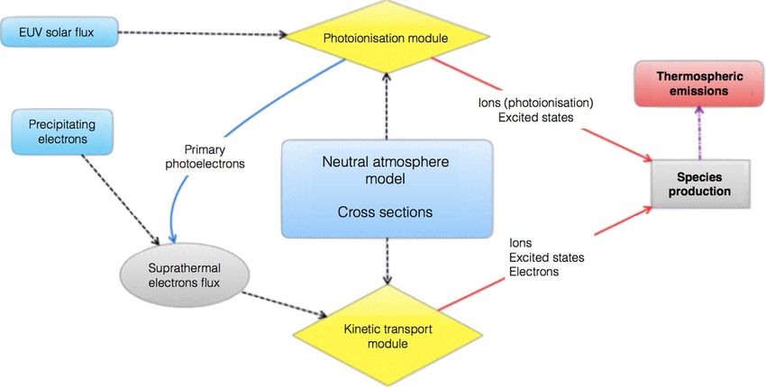
M. Barthelemy et al.: J. Space Weather Space Clim. 2018, 8, A44

an economically attractive CubeSat platform (Hevner &                  sight can be applied to enable their registration. In this case
Holemans, 2011). This ATISE instrument will be able to regis-          the highest line of sight reaches up to about 338 km.
ter the vertically-resolved spectral emissions of auroras from              Since the main goal of the instrument is to both monitor
the spacecraft in a LEO.                                               and study the auroral emissions, an almost polar orbit is
    The ATISE spectrometer has been designed with a spectral           mandatory. A sun synchronous orbit could then be an interest-
coverage from 400 to 900 nm and resolving power of 500 (i.e.           ing choice especially for monitoring the cusp and a part of the
1 nm at 500 nm), to enable the resolution of the vibrational           auroral oval. However, these orbits have a fixed orbital plane in
structure of the molecular emission. Resolving the rotational          terms of the local hour. This does not allow studying the
structure, i.e. reaching a resolution of a few cm1, is not within     physics associated with changing local hour, which is extre-
reach of the lSPOC instrument, considering that different              mely important especially regarding the magnetosphere-
electronic states of the N2 molecule have rotational constants         thermosphere coupling. For this reason we choose an orbit with
between 1 and 2 cm1; at least not within the available volume         a much lower than 90, but higher than 70, inclination, in
of a CubeSat.                                                          order to be able to monitor the auroral oval and the cusp. Local
    In terms of sensitivity, the objective is to detect a number of    hour shift is then slow. At an inclination of 75, a 12 h shift
more or less faint molecular emissions, including vibronic             takes 60 days at an orbit altitude of 650 km, resulting in a
transitions belonging to, among others, Nþ    2 , N2 and potentially   complete view of all local hours every 2 months.
O2. We require that the detection threshold is no higher than               The airglow is much fainter than the auroral emissions. Two
5 R1 and that the sensitivity2 is at least 1 R for a 1-second          observation modes are thus planned with exposure time of 1 s
exposure time. Considering the very large range of intensities         in auroral regions and 20 s in airglow regions, with a latency of
of auroral emissions, a dynamic range exceeding 103 is                 1 s in both modes. The switch between these two modes will be
required.                                                              automatic and based on auroral oval simulations based on the
    With a height of 100 mm and a footprint of less than               Kp parameters using the NOAA (National Oceanic and
200 mm by 300 mm, the instrument payload then fits in a                Atmospheric Administration) auroral simulation package
6 U CubeSat frame. Including the bus, the entire satellite will        OVATION (Newell et al., 2014) or the Sigernes et al. (2011)
adhere to the 12U CubeSat standard.                                    model. These two simulations give previsions of Kp over
    In the red and near infrared, OH exhibits some strong emis-        3 days, which means that telemetry commands will have to
sion lines. These are particularly prominent at altitudes between      be sent to the satellite at least once every 3 days.
80 and 90 km (Sheese et al., 2014). Since the focus of our                  The data rate produced by the experiment will be about 1.5
instrument is the observation of auroral and airglow emissions         Gbit/day based on the assumption of six spectra every 2 s in
in the thermosphere and ionosphere, we choose by default the           the auroral region and many fewer in the airglow region (2–4
lowest line of sight at an altitude of 100 km. If the altitude of      images per orbit). Since the auroral monitoring sequences for
the satellite is around 650 km, this means that each FoV has a         each orbit are linked with Kp, the data rate increases when
vertical extent of a bit less than 50 km at the limb configura-        magnetic activity increases, reaching 2.5 Gbit/day for Kp = 7.
tion (47.7 km with a spherical Earth hypothesis). This means                The planned nominal mission duration of 2 years long will
that the higher line of sight is between 338 and 386 km, and           be extended to 5 years if the instrument and the satellite are
therewith much higher than the red line emission peak which            still working. The altitude of the orbit has been chosen to allow
is found at around 230 km, even if we consider the very large          for a 5 years mission. In this case, this will cover almost one
vertical extent of the red line profile (Megan-Gillies et al.,         half of a solar cycle to allow a monitoring of a large range
2017). These parameters define the ADCS (Acquisition                   of solar conditions. Some specific observational modes of oper-
Determination and Control System) performance required to              ation will be implemented. One will slightly tilt the satellite to
assure that the spectrometer correctly aims at the same auroral        lower the lines of sight to enable observation of previously
region during the exposure time (of the order of 1 s) without          mentioned OH emissions. This will be performed during night-
risk of including the strong OH emissions in its FoV. This             glow observations.
means that the pointing accuracy and stability need to be better
than respectively, 0.1 and 0.02 s1. CubeSat ADCS that meet          3.3 Optical design
such accuracy and stability requirements are commercially
available in the form of the Blue Canyon X-ACT50 system                    In order to satisfy the mission requirements, the optical
(with, as of 2018, flight heritage going back to its smaller cou-      design has to meet the following two conditions:
sin the XACT-15) or the Hyperion ADCS-400 system. In our                   Produce six line of sight detection channels, each covering
case, the ATISE system and platform, including the ADCS,               1.5 (horizontal) by 1 (vertical) FoV. At the limb, each line of
will be realized by the Toulouse University Space Center               sight will cover around 47 km in altitude with a small gap of
(CSUT) and commercial ADCS will not be used except as                  5 km between each line of sight due to the mounting frame
backup solution.                                                       of the six microlenses.
    During the nightside of the orbit, observations of the OH              The image of the entrance pupil needs to be projected onto
emissions could also be of scientific interest by themself. In this    each detector, ensuring a homogeneous illumination of each
case, a small tilt of the satellite corresponding to one line of       one of the six detection devices (Gillard et al., 2012; Le Coarer
                                                                       et al., 2014). In order to save space in the instrument, three
                                                                       physical detectors (Pyxalis HDPYX) are used to record the
 1
   1 R represents 106 ph cm2 s1 in 4n steradian; See Bake (1974)     six spatial interferograms associated with the six lines of sight.
for more information.                                                  For this, one line of sight illuminates one half of one physical
 2
   Smallest detectable variation in intensity.                         detector.

                                                               Page 4 of 12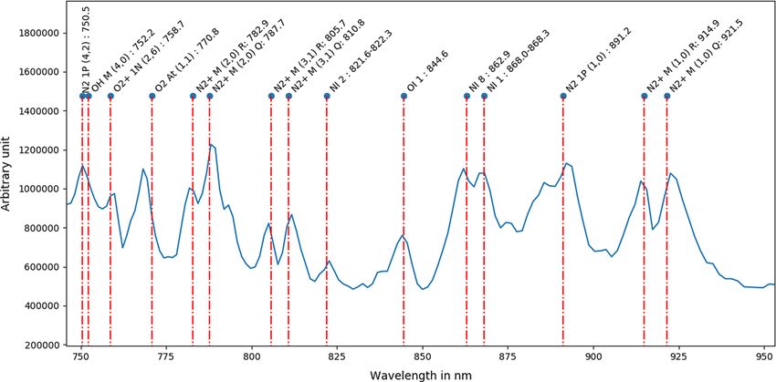
M. Barthelemy et al.: J. Space Weather Space Clim. 2018, 8, A44

Fig. 2. Optical design of the ATISE instrument. The grey plate represents 6U size.

    The combination of these two conditions requires beam             as ROLO for Robotic Lunar Observatory. The French space
shaping optics with a rather long, folded, optical beam path that     agency created a similar tool called POLO for Pleiades Orbital
consumes about 4U of the available space. The optical design          Lunar Observations (Lacherade et al., 2014; Xiong et al.,
that was retained, has an entrance lens with a focal distance of      2014). The precision achievable with the ROLO and POLO
about 686 mm, producing an image of the FoV on a micro-lens           models is of the order of 10% in absolute calibration and 1%
array consisting of six lenses, placed in the focal plane of the      in relative calibration (Goguen et al., 2010). These calibrations
entrance lens (Fig. 2). Subsequently, each micro-lens produces        cannot be carried out during all phases of the moon. Exact full
the image of the entrance lens on the corresponding detector.         moon is forbidden due to an increase in the intensity that is
Finally, three plane mirrors fold the optical beam path in the        poorly simulated by both ROLO and POLO. Periods between
available space.                                                      first quarter, new Moon and last quarter are also forbidden
                                                                      because too imprecise. Favorable periods are around full moon.
3.4 Calibration                                                       One or two calibrations are planned each month.
                                                                           Moreover, it will also be necessary to calibrate the interfer-
    During the mission, the instrument is very likely to experi-      ograms on very simple spectra, preferably without molecular
ence a performance degradation due to exposure to, among              emission. This will result in a simple interferogram that can
other effects, radiation in space, outgassing, and dust. It is thus   be used to calibrate the OPDs for each of the detector’s pixels,
necessary to regularly calibrate the spectrometer in order to         which could change with the environmental conditions. The
maintain an absolute photometry of each line and to enable a          easiest way to achieve this is to rotate the satellite by 90 with
quantitative comparison to the results of simulations with the        respect to normal operation and to aim all six lines of sight
kinetic code. Calibration of ground based instruments have            (now horizontal) at one altitude in the upper part of the vertical
been made using point sources like stars (Grubbs et al.,              range. The interferogram will then belong to the spectrum com-
2016). Since the instrument is looking at a spatially extended        prised of the three red lines, belonging to the O1 D – O3P triplet
source, it is more convenient to perform the calibration using        (at 630, 636, and 639 nm), which exhibit a constant intensity
extended sources, with very constant photometric flux over            ratio only controlled by the Einstein coefficients. The 639 nm
the mission duration. The Moon is a unique reference source           line is very faint and will normally be hardly visible, if at all.
that meets the above requirements (Teillet et al., 2007). The
lunar reflectance is unmatched in its stability, which is better
than 10 ppb over one year (Kieffer, 1997). Its radiance is
similar to sunlit landmasses, but can be known with much
                                                                      4 Imaging: AMICal Sat and ATISE imager
higher precision (
M. Barthelemy et al.: J. Space Weather Space Clim. 2018, 8, A44
lines of sight can be in and the others out of such an arc. In Despite the fact that the sun synchronous orbit (SSO) is not
order to have information on the scene being observed it is thus totally satisfactory since there is no shift in local hour, this orbit
necessary to use an imager in addition to the spectrometer. is more easily accessible due to a larger number of launch
Moreover, an imager with a better vertical resolution than the opportunities. All SSOs with a local hour equal to 12 h ± 4 h
ATISE instrument is a way to interpolate the data within each will be acceptable, with a preference for the 10h30–22h30 local
line of sight of the spectrometer, which will enable increasing hour. The final choice will be determined by the launch
the vertical resolution of the entire mission. This requires an opportunities.
on-board intensity calibrated imager with a FoV larger than that AMICal Sat measurements can be synchronized with those
of the spectrometer total FoV, i.e. larger than i.e. 6 · 1.5. The provided by the Russian Meteor M2 satellite (Asmus et al.,
imager data will also have to be calibrated. Since we require an 2014; Kalegaev et al., 2018). The orbit of Meteor M2 is an
absolute photometry precision of 10%, a Signal-to-Noise-Ratio SSO at an altitude of about 800 km altitude. It has on-board
(SNR) higher than 10 is necessary. To take into account a meteorological instruments, including detectors developed at
potential degradation of the instrument during the mission, MSU. One of the detectors measures fluxes of keV charged
we impose an initial SNR exceeding 20. particles. Comparison of AMICal Sat and Meteor M2 measure-
Within the detectors that meet these specifications, we ments in magneto-conjugate regions will enable obtaining more
choose the Onyx by Teledyne E2V 1.3 Mpix detector with a information on mechanisms of auroral particle precipitations.
pixel size of 10 lm. This detector is particular in that it is a AMICal Sat will use the S-band for data transmission,
sparse RGB (Red, Green, Blue) detector with 1 RGB pixel meaning it will necessarily take fewer pictures than ATISE.
and 15 B&W (Black and White) pixels out of every 16 pixels. As for ATISE, recording will be limited to the auroral oval only.
The required short exposure time will necessitate a large The extent of the auroral oval will be estimated based on Kp
aperture objective and the available volume in the 6U dedicated forecast values. To limit the number of pictures and therewith
for the payload will only allow for a short focal length. the data rate, images registration frequency will be lower than
An objective between 17 mm and 35 mm reaches the require- in the ATISE case. A superposition of 1/3 of each photo,
ment if the aperture is f/1.4, or better still f/0.95. In these con- regarding the previous one, is then planned in nadir mode. This
figurations, the FoV of the imager is between 50 and 26, will allow to both set positioning of the satellite during images
which meets our requirement of exceeding the spectrometer recording and to limit the number of images. In limb mode, one
FoV.3 picture every 30 s is planned instead of one every 2 s. Data
The images will be compressed on board. Taking images at production is then limited to around 250 Mbits per day.
the same rate as the spectrometer, they will represent the main
part of the data volume. The total data volume will reach
around 6 Gbit per day which is still acceptable in LEO for
5 ATISE ground-based demonstration:
X-band data transmissions.
2017 campaign in Skibotn
4.2 AMICal Sat mission 5.1 Observation condition
An imager as described above is by itself an interesting Since the ATISE concept has never been tested for auroral
instrument to study auroral phenomena from a space weather emissions, a ground-based demonstrator was built and tested in
point of view, especially if nadir observations are added. This Skibotn (Norway) at the end of February, beginning of March,
consideration has led us to define a spin-off mission that will 2017. The optical design was identical to that of the space
embark an auroral imager in a 2U cubesat. In addition to the payload design, except for the fact that only one half detector
limb observation foreseen for the ATISE mission, nadir obser- was active meaning that only one line of sight was registered.
vation will be performed. This will enable mapping the spatial Also, the detector proximity electronics were different from
extend of the oval and distinguishing its internal structure. With those of the future satellite electronics. The instrument was
the detector and objective as defined for the ATISE mission, a installed in the Skibotn observatory cupola (20210 5400 E,
spatial resolution better than 2 km at an altitude of 110 km is 69200 5400 N). During the first 3 days of the campaign, it looked
achievable. The limb observation of the aurora will enable con- toward the West with an elevation angle of 30, while the
structing vertical intensity profiles, comparable to those that remaining time it looked toward the East (same elevation
will be obtained with the ATISE imager. However the ADCS angle).
system that will be used in the AMICal 2U CubeSat, is much During the first two observation nights, the exposure time
more basic. This will necessarily lead to image degradation was 4 s as the optical system was not totally optimized. The
(blurring) due to both satellite speed and pointing errors. The exposure time was subsequently reduced to 2 s.
first source of image blurring is well known, and can be
corrected for, provided the SNR is sufficiently high.
AMICal Sat will also test the lunar calibration procedure
using the Moon as a reference source that should lead to 5.2 Results
absolute photometric data with 10% accuracy and 1% preci-
sion. AMICal Sat is expected to be launched during the first Figure 3 shows a spectrogram of data collected during
trimester of 2019 for a 1-year mission, extendable to 3 years. almost 10 h on March 1. Wavelength is shown on the vertical
axis, while time is on the horizontal axis. The intensity of the
3
The final design has converged to a focal length of 23 mm with an spectra is color coded. The green line emission is easily recog-
aperture of f/1.4. nizable in all spectra recorded throughout the night. A large
Page 6 of 12M. Barthelemy et al.: J. Space Weather Space Clim. 2018, 8, A44
900
730
Wavelength (nm)
560
480
400
370
20:00 23:30 02:00 04:30
Local hours
Fig. 3. Spectrogram of a series of spectra collected during the almost 10 hours of observation in March 2017. Wavelength (in nm) is on the
vertical axis and the local time is on the horizontal axis. The red and green lines are easily recognizable at respectively 557 and 630 nm. The
two N+ lines at 391 and 428 nm are faint but recognizable. The N2 first positive and N+ Meinel features are present in the red part of the
spectra (see also Fig. 4). The dawn at the end of night is also recognizable at the right of the figure. The wavelength scale of the figure is
approximate and does not correspond exactly to the fit mentioned in the text. Some strong enhancements of the total intensity are visible.
These enhancements seem to concern all wavelengths. This appears to be some combination of different effects: A strong enhancement of all
line intensities that is real and due to greater auroral activity. However, since the intensity scale is the same for the entire night, the noise
becomes much larger when the total number of photons increases, giving the impression of continuous emissions. This is of course a fake
process exacerbated by the strong noise experienced during the ground based demonstration. A third effect is due to the Fourier transform
process, despite the apodisation windows used. These data processing effects will be resolved by ground based calibrations.
group of intense lines is present in the red, including the are clearly present and easily assigned, it is more difficult to
oxygen red line (630 nm) and the line at 844.6 nm correspond- assign the features between 630 and 700 nm where lines of
ing to the atomic oxygen 3p3P–3s3S transition. In the blue and the N2 first positive bands should be present.
near UV, the most visible features are the N þ2 bands of the first One important point is the stability of the spectrometer in
negative system (B2 Rþ 2 þ
u X Rg ) at 391 (0–0) and 427 nm terms of sensitivity and wavelength calibration. We have
(0–1). To facilitate the identification of the other spectral fea- several means to characterize these. Firstly, some lines such
tures, a wavelength calibration was performed by fitting a as the 630-nm and 636-nm lines of O I or the 427-nm and
polynomial to the positions of the 427.8, 577.7, 630.0 and 391-nm lines of N+ must have a constant intensity ratio since
844.6 nm lines. We used a third order polynomial with the they share the same upper level. Secondly, we can compare
following parameters: our spectra with those obtained by another instrument, the
‘‘premier cru’’ spectropolarimeter that was operated during
P ðxÞ ¼ 3:747 107 x3 3:923 104 x2 the same time frame and on the same line of sight.
þ 2:067 101 x þ 9:168 103 : ð1Þ In order to achieve this, the intensities of each line must be
determined. For the prototype of ATISE, we can fit Gaussian
profiles to the visible features and use the fitted line areas,
With this fit the identification of the principal lines is quite numerically integrate the line profiles to obtain their intensity,
satisfactory as shown in Figure 4 for the red part of the spectra. or use the center line intensity for each feature (effectively
Lines from both the N2 first positive band and the Nþ 2 Meinel assuming that all lines have the same width). This hypothesis
band are correctly identified. While emissions above 700 nm and the fact that some significant overlaps occur make the latter
Page 7 of 12M. Barthelemy et al.: J. Space Weather Space Clim. 2018, 8, A44
Fig. 4. Section of the spectrum between 750 nm and 930 nm averaged over one night (March 1, 2017). Identification of the lines is given at
the top of the figure.
two options problematic. We therefore proceed with a fit of The noise is larger than expected. An analysis after the cam-
multiple Gaussian profiles to the spectra. paign showed that a grounding error (ground loop) in the prox-
Following the NIST data and Baluja & Zeippen (1988), the imity electronics increased the noise level. This error has been
ratio I630/I636 should be slightly larger than 3. The ratio is, how- corrected and will thus not affect the space version of these
ever, clearly higher for the ATISE data. It reaches 4.2 for the electronics. The ground loop error does explain why it was
data of March 1 and 3.7 for the data of March 4. The impossible to record good spectra with a 1-second exposure
636 nm line is not detectable in the data of March 2. As for setting during the test campaign.
the 427-nm to 391-nm line intensity ratio, the theoretical The test campaign thus clearly revealed some problems
branching ratio (Torr & Torr, 1982) is 0.35. It is clear that in with the spectrometer that need to be addressed. The electron-
the ATISE data this ratio is not respected. This is however ics problem has been identified and corrected after the cam-
easily explained since the sensitivity of the detector is falling paign, whereas calibration issues with the spectrometer will
strongly between 427 nm and 391 nm, mostly due to the vary- be corrected by using backside illuminated detectors and
ing reflectivity of the detector surface. This reflectivity is higher proper data processing procedures.
in the red resulting in a higher sensitivity in that part of the In general, the tests show that the ATISE instrument is able to
spectrum. Moreover, small irregularities at the surface of the record spectra with a SNR that is sufficient for the auroral obser-
detector, due to the passivation layer, can perturb the interfero- vations. The instrument was also shown to be sufficiently stable
grams and this may well explain the observed discrepancy in terms of both sensitivity and wavelength calibration to enable
between previously determined line intensities and those mea- identification of all major features in the recorded spectra.
sured by the ATISE demonstrator. This will be corrected using
two different strategies:
6 Coupling with the Transsolo code for space
– Instead of using frontside illuminated detectors, ATISE weather applications
will use backside illuminated detectors. This solution will
reduce the irregularities mentioned above by allowing a
After solving the previously mentioned issues, fully cali-
thinner passivation layer and then remove their effect from
brated spectra of the aurora will allow retrieving some space
the interferograms. This is also expected to partially solve
weather parameters through modeling of notably the particle
the drastic reduction of the sensitivity in the blue and near-
precipitation fluxes. The simulation results can also be com-
UV regions.
pared to those measured directly at 800 km altitude by the
– An additional correction will be added to the data process-
Meteor-M2 satellite.
ing by calibrating the spectrometer on the ground using
spectral calibration lamps with known intensity ratios.
6.1 Interpretation of the data
Regarding the requirements in terms of sensitivity, it is Altitude resolved spectra can be interpreted using
clear that the 5 R detection sensitivity threshold is not reached. kinetic codes that calculate the light emissions based on an
Page 8 of 12M. Barthelemy et al.: J. Space Weather Space Clim. 2018, 8, A44
Fig. 5. Schematic view of the Transsolo simulation flow. Inputs are in blue and output in red.
atmospheric model and the energetic inputs like solar UV flux a more complete characterization of the system. It will, how-
and particle precipitations. Several of these models exist, some ever, be necessary to limit the number of explored parameters,
with bi-directional flux calculation (up and down fluxes), others compared to the number of input parameters of the code. It is
with multi stream calculations. The model to be used with the clear that priority will be given to the energy distribution and
ATISE and AMICal data will be the Transsolo code total flux of the precipitating particles, which is similar to the
(Lummerzheim & Lilensten, 1994; Lilensten & Blelly, 2002) parameters explored by Strickland et al. (1989). Since we use
developed over the last 25 years to calculate the vertical trans- independent atmospheric models (MSIS or IRI), we will a pri-
port of the particles through the thermosphere and the associ- ori avoid to use the scaling factor linked to the atomic oxygen
ated light emissions. The code has recently been used to profile. However, considering only one particle distribution is
calculate the NO emissions in auroral regions (Vialatte et al., often not sufficient to characterize the particle precipitation,
2017). The Transsolo code is a multi-stream kinetic code that especially since the magnetospheric sources can be multiple.
allows from inputs such as the solar EUV flux and the electron The inversion procedure will then allow to superimpose several
precipitation to calculate the emissions. It is a 1D code mean- distributions. The shape of the distribution will also be investi-
ing that all calculations are done along an axis which is often gated using a limited number of pre-determined shapes
the magnetic field line. A schematic overview of the Transsolo (Gaussian, Maxwellian, etc.). In a first stage, by using multiple
flow is presented in Figure 5. This code takes the atmospheric direct runs of the code, a positioning of the measured results in
model as an input. In our case, two models are useable: the input parameter space will be feasible, and will allow for
NLRMSISE 2000 (Picone et al., 2002) or IRI (Bilitza et al., the interpretation of the data in a reasonable amount of time.
2012). However, a study of a proper inversion procedure of the data
is ongoing and will be finalized before the ATISE satellite
6.2 Spectroscopic data launch in 2021. Strategies like those used by Simon Wedlund
et al. (2013) based on the multiplicative algebraic reconstruc-
It is first clear that the recorded intensities for each line of tion technique or the maximum entropy method could be
sight do not only comprise the intensities of the auroral adapted since the forward model is similar. A first version will
emissions at the tangent point of the line of sight, but actually be tested on an AMICal Sat dataset.
integrate all emissions, also those from higher altitude atmo-
spheric layers since the satellite will fly at 650 km. This means 6.3 Imaging data
that some O I red line emissions will be visible, even for the
lowest line of sight. Concerning the interpretation of the data The limb image data by themselves will be interesting for
with the Transsolo code this means that several simulations space weather studies, but the amount of information that they
corresponding to different geographical positions will be can provide is limited. In a first processing step, only the total
required, especially for the lowest line of sight. Since the Trans- intensities of the vertical profile will be used. In a second step,
solo code is a 1D code, the only way to accomplish this is by the sparse RGB information will be processed. This means that
running it several times using the hypothesis of negligible if interpretation of the limb data of AMICal Sat will be carried
horizontal transport. out using the Transsolo code, it is likely that the solution is
The advantage of a large band spectrometer is to enlarge ill-determined, especially when not using the RGB information
the number of emission lines and bands accessible; enabling in the first processing step. However, since Space Weather is a
Page 9 of 12M. Barthelemy et al.: J. Space Weather Space Clim. 2018, 8, A44
Fig. 6. Aurora image taken with the demokit of the ONYX detector during the Ny-Ålesund Nov 2017 campaign. The exposure time is 0.82 s,
the analog gain is ·6. The instrument was inclined at about 45. The aurora was faint, barely visible with naked eyes.
multi-instrument and multi-measurement science, some regarding the space mission requirements are resolved and
coordinated measurements will be possible with some ground some improvements in both hardware (noise reduction, back-
based instruments such as the EISCAT radars, which give the side illumination) and data processing are still needed. The
state of the ionosphere along the radar line of sight, or with ATISE and AMICalSat missions are expected to deliver a very
optical instruments such as the ALIS cameras. large set of data for a large variety of space weather studies.
For nadir imaging, observation of the oval is by itself extre- Vertical profiles will enable the reconstruction of the altitude
mely interesting since it gives a direct mapping of the magnetic at which the dominant emissions take place, and constraints
field lines that affect the particle precipitations. This will be on the particle precipitation up to few keV. These particles
extremely useful for the magnetosphere-ionosphere coupling are not the most energetic ones, but by their abundance, they
study, giving a more precise idea of the location of radiation play a major role in the thermosphere-ionosphere dynamics.
belt regions and of subsequent magnetosphere processes. Small The fast time response of the instruments will enable recon-
scale structure of the size of a few kilometers in a short obser- structing dynamics with good accuracy. Before the launch of
vation time will be visible, and will allow for a much better the satellites, several additional ground based campaigns will
comprehension of the dynamics of the particle precipitations. be performed with both the imagers and the spectrometer.
A black and white prototype of the imager have been tested The ATISE spectrometer will be tested again during a
in November 2017, in Ny-Ålesund (Spitzberg, Norway). An campaign planned for the 2019 winter. Data on particle precip-
objective with a focal length f = 17 mm and a numerical aper- itations obtained during the ATISE flight campaign will be
ture of f/1.4 has been fitted to a demo-kit of the Teledyne-E2V compared with measurements of low-energy electron fluxes
ONYX detector. An image taken during this campaign is made by Meteor-M2 or similar LEO satellites. We also plan
shown in Figure 6. The main conclusion of this campaign is to make sure that the ATISE mission will coincide with
that the imager configuration is sensitive enough for faint auro- measurement campaigns of particle instruments, such as the
ras with exposure times of the order of 1 s, thus validating the Dynagrad developed by ONERA, or similar auroral electron
instrument concept. detectors included in the ‘‘UniverSat Socrat’’ mission currently
developed by the Moscow State University (Panasyuk et al.,
2017). The two satellites will be included in this large multi-
7 Conclusions satellite mission dedicated to Space Situational Awareness
(SSA).
As stated in the previous paragraphs, the demonstration of As to the future prospects of ATISE, we mention that it
the ATISE prototype is convincing, even though not all issues would be extremely interesting to fly multiple ATISE satellites
Page 10 of 12M. Barthelemy et al.: J. Space Weather Space Clim. 2018, 8, A44
in a constellation in order to increase both spatial and temporal Gillard F, Ferrec Y, Guérineau N, Rommeluère S, Taboury J, Chavel
coverage, as would be the development of a hyperspectral P. 2012. Angular acceptance analysis of an infrared focal plane
version of the ATISE spectrometer. array with a built-in stationary Fourier transform spectrometer.
J Opt Soc Am A 29: 936. DOI: 10.1364/JOSAA.29.000936.
Acknowledgements. The AMICal Sat and ATISE missions Goguen JD, Stone TC, Kieffer HH, Buratti BJ. 2010. A new look at
are being developed by the CSUG and MSU/SINP, in photometry of the Moon. Icarus 208: 548–557. DOI: 10.1016/
collaboration with the CSUT and SMC TC. CSUG is funded j.icarus.2010.03.025.
by Air Liquide Advance Technologies, Teledyne E2 V, Nico- Grubbs G, Michell R, Samara M, Hampton D, Jahn J-M. 2016. A
matic, Sofradir and Gorgy Timing through the UGA Founda- synthesis of star calibration techniques for ground-based narrow-
tion. The MSU/SINP team was supported by RFBR grant band electron-multiplying charge-coupled device imagers used in
16-05-00760. Educational aspects have been partly funded auroral photometry. J Geophys Res (Space Phys) 121: 5991–6002.
by the IDEX in Grenoble. The ATISE prototype has been DOI: 10.1002/2015JA022186.
funded by the Auvergne Rhone Alpes region. This work Hecht JH, Strickland DJ, Conde MG. 2006. The application of
was partly supported by the Programme National PNST of ground-based optical techniques for inferring electron energy
CNRS/INSU co-funded by CNES and by CNES. The editor deposition and composition change during auroral precipitation
thanks Johan De Keyser and an anonymous referee for their events. Journal of Atmospheric and Solar-Terrestrial Physics 68:
assistance in evaluating this paper. 1502–1519. DOI: 10.1016/j.jastp.2005.06.022.
Hevner R, Holemans W. 2011. An Advanced Standard for CubeSats,
Paper SSC11-II-3. In: 25th Annual AIAA/USU Conference on
Small Satellites, SSC11-II-3.
References Kaeppler SR, Hampton DL, Nicolls MJ, Str0mme A, Solomon SC,
Hecht JH, Conde MG. 2015. An investigation comparing ground-
Asmus VV, Zagrebaev VA, Makridenko LA, Milekhin OE, Solov’ev based techniques that quantify auroral electron flux and
VI, Uspenskii AB, Frolov AV, Khailov MN. 2014. Meteorological conductance. J Geophys Res (Space Phys) 120: 9038–9056.
satellites based on Meteor-M polar orbiting platform. Russ Meteorol DOI: 10.1002/2015JA021396.
Hydrol 39(12): 787–794. DOI: 10.3103/S1068373914120012. Kalegaev VV, Barinova WO, Myagkova IN, Eremeev VE,
Baker DJ. 1974. Rayleigh, the unit for light radiance. Appl Opt 13: Parunakyan DA, Nguyen MD, Barinov OG. 2018. Empirical
2160–2163. DOI: 10.1364/A0.13.002160. model of the high-latitude boundary of the Earth’s outer radiation
Baluja KL, Zeippen CJ. 1988. M1 and E2 transition probabilities for belt at altitudes of up to 1000 km. Cosm. Res. 56(1): 32–37.
states within the 2p4 configuration of the O I isoelectronic DOI: 10.1134/S0010952518010069.
sequence. J Phys B: At Mol Phys 21: 1455–1471. DOI: 10.1088/ Kauristie K, Pulkkinen TI, Amm O, Viljanen A, Syrjasuo M, et al.
0953-4075/21/9/007. 2001. Ground-based and satellite observations of high-latitude
Bilitza D, Brown SA, Wang MY, Souza JR, Roddy PA. 2012. auroral activity in the dusk sector of the auroral oval. Ann
Measurements and IRI model predictions during the recent solar Geophys 19: 1683–1696. DOI: 10.5194/angeo-19-1683-2001.
minimum. J Atmos Sol Terr Phys 86: 99–106. DOI: 10.1016/ Kieffer HH. 1997. Photometric Stability of the Lunar Surface. Icarus
j.jastp.2012.06.010. 130(2): 323–327. DOI: https://doi.org/10.1006/icar.1997.5822.
Birn J,Artemyev AV, Baker DN, Echim M, Hoshino M, Zelenyi LM. Lacherade S, Aznay O, Fougnie B, Lebegue L. 2014. POLO: a unique
2012. Particle Acceleration in the Magneto tail and Aurora. Space dataset to derive the phase angle dependence of the Moon
Sci Rev 173: 49–102. DOI: 10.1007/s11214-012-9874-4. irradiance. In: Sensors, Systems, and Next-Generation Satellites
Broadfoot AL, Hatfield DB, Anderson ER, Stone TC, Sandel BR, XVIII, vol. 9241 of Proc. SPIE, 924112. DOI: 10.1117/12.2067283.
Gardner JA, Murad E, Knecht DJ, Pike CP, Viereck RA. 1997. N2 Le Coarer E, Guerineau N, Martin G, Rommeluere S, Ferrec Y,
triplet band systems and atomic oxygen in the dayglow. J Geophys Schmitt B. 2014. SWIFTS-LA: an unprecedently small static
Res 102: 11567–11584. DOI: 10.1029/97JA00771. imaging Fourier transform spectrometer. In: Proc. SPIE 10563,
Christensen AB, Paxton LJ, Avery S, Craven J, Crowley G. 2003. International Conference on Space Optics – ICSO 2014, 105634J,
Initial observations with the Global Ultraviolet Imager (GUVI) in 17 November 2017. DOI: http://dx.doi.org/10.1117/12.2304159
the NASA TIMED satellite mission. J Geophys Res (Space Phys) Lilensten J, Blelly PL. 2002. The TEC and F2 parameters as tracers
108: 1451. DOI: 10.1029/2003JA009918. of the ionosphere and thermosphere. J Atmos Sol Terr Phys 64:
Cisek M, Makuch P, Petelski T. 2017. Comparison of meteorological 775–793. DOI: 10.1016/S1364-6826(02)00079-2.
conditions in Svalbard fjords: Hornsund and Kongsfjorden. Lilensten J, Moen J, Barthelemy M, Thissen R, Simon C, Lorentzen
Oceanologia 59(4): 413–421. DOI: https://doi.org/10.1016/ DA, Dutuit O, Amblard PO, Sigernes F. 2008. Polarization in
j.oceano.2017.06.004, URLhttp://www.sciencedirect.com/science/ aurorae: A new dimension for space environments studies.
article/pii/SQQ783234173QS672. Geophys Res Lett 35: L08804. DOI: 10.1029/2007GL033006.
Diard T, de la Barriere F, Ferrec Y,Guerineau N, Rommeluere S, Lummerzheim D, Lilensten J. 1994. Electron transport and energy
Le Coarer E, Martin G. 2016. Compact high-resolution micro- degradation in the ionosphere: Evaluation of the numerical
spectrometer on chip: spectral calibration and first spectrum. In: solution, comparison with laboratory experiments and auroral
Micro- and Nanotechnology Sensors, Systems, and Applications observations. Ann Geophys 12: 1039–1051. DOI: 10.1007/
VIII, vol. 9836 of Proc. SPIE, 98362W. DOI: 10.1117/12.2223692 s00585-994-1039-7.
Germany GA, Spann JF, Parks GK, Brittnacher MJ, Elsen R, Chen Megan-Gillies D, Knudsen D, Donovan E, Jackel B, Gillies R,
L, Lummerzheim D, Rees MH. 1998. Auroral Observations from Spanswick E. 2017. Identifying the 630 nm auroral arc emission
the POLAR Ultraviolet Imager (UVI). Washington DC American height: A comparison of the triangulation, FAC profile, and
Geophysical Union Geophysical Monograph Series 104: 149. electron density methods. J Geophys Res (Space Phys) 122:
DOI: 10.1029/GM104p0149. 8181–8197. DOI: 10.1002/2016JA023758.
Page 11 of 12M. Barthelemy et al.: J. Space Weather Space Clim. 2018, 8, A44
Newell PT, Liou K, Zhang Y, Sotirelis T, Paxton LJ, Mitchell EJ. Stone TC, Kieffer HH. 2004. Assessment of uncertainty in ROLO
2014. OVATION Prime-2013: Extension of auroral precipitation lunar irradiance for on-orbit calibration Barnes WL, Butler JJ
model to higher disturbance levels. Space Weather 12: 368–379. (Eds.). Earth Observing Systems IX, vol. 5542 of Proc. SPIE,
DOI: 10.1002/2014SW001056. 300–310. DOI: 10.1117/12.560236
Panasyuk MI, Podzolko MV, Kovtyukh AS, Brilkov IA, Vlasova NA, Strickland DJ, Meier RR, Hecht JH, Christensen AB. 1989.
Kalegaev VV, Osedlo VI, Tulupov VI, Yashin IV. 2017. Optimiza- Deducing composition and incident electron spectra from
tion of measurements of the Earth’s radiation belt particle fluxes. ground-based auroral optical measurements. I – Theory and
Cosm. Res. 55: 79–87. DOI: 10.1134/S0010952516060071. model results. II – A study of auroral red line processes. III –
Picone JM, Hedin AE, Drob DP, Aikin AC. 2002. NRLMSISE-00 Variations in oxygen density. J. Geophys. Res. 94: 13527–13539.
empirical model of the atmosphere: Statistical comparisons and DOI: 10.1029/JA094iA10p13527.
scientific issues. J Geophys Res (Space Phys) 107: 1468. DOI: Teillet PM, Barsi JA, Chander G, Thome KJ. 2007. Prime candidate
10.1029/2002JA009430. Earth targets for the post-launch radiometric calibration of space-
Rommeluere S, Guerineau N, Haidar R, Deschamps J, de Borniol E, based optical imaging instruments. In Earth Observing Systems
Million A, Chamonal J-P. 2008. Chamonal, and Destefanis. XIIIn: Earth Observing Systems XII. vol. 6677 of Proc. SPIE,
Infrared focal plane array with a built-in stationary Fourier- 66770S. DOI: 10.1117/12.733156
transform spectrometer: basic concepts.Opt Lett 3(3): 1062. DOI: Torr MR, Torr DG. 1982. The role of metastable species in the
10.1364/OL.33.001062. thermosphere. Rev Geophys Space Phys 20: 91–144.
Saito H, Hirahara M, Mizuno T, Fukuda S, Fukushima Y, et al. 2011. Tuttle S, Gustavsson B, Lanchester B. 2014. Temporal and spatial
Small satellite REIMEI for auroral observations.Acta Astronaut evolution of auroral electron energy spectra in a region surround-
69(7): 499–513. DOI: https://doi.org/10.1016/j.actaastro.2011.05. ing the magnetic zenith. J Geophys Res (Space Phys) 119:
007. 2318–2327. DOI: 10.1002/2013JA019627
Sheese PE, Llewellyn EJ, Gattinger RL, Strong K. 2014. OH Meinel Vialatte A, Barthelemy M, Lilensten J. 2017. Impact of Energetic
band nightglow profiles from OSIRIS observations. J Geophys Electron Precipitation on the Upper Atmosphere: Nitric
Res (Atmos.) 119: 11. DOI: 10.1002/2014JD021617. Monoxide. Open Atmos Sci J 11: 88–104. DOI: 10.2174/
Sigernes F, Dyrland M, Brekke P, Chernouss S, Lorentzen DA, 1874282301711010088
Oksavik K, Sterling Deehr C. 2011. Two methods to forecast Wagner SC, Hewison T, Stone T, Lacherade S, Fougnie B, Xiong X.
auroral displays. J Space Weather Space Clim 1(27): A03, 2015. A summary of the joint GSICS – CEOS/IVOS lunar
DOI: 10.1051/swsc/2011003. calibration workshop: moving towards intercalibration using the
Simon Wedlund C, Lamy H, Gustavsson B, Sergienko T, Moon as a transfer target. In: Sensors, Systems, and Next-
Brändström U. 2013. Estimating energy spectra of electron Generation Satellites XIX, vol. 9639 of Proc. SPIE, 96390Z. DOI:
precipitation above auroral arcs from ground-based observations 10.1117/12.2193161.
with radar and optics. J Geophys Res (Space Phys) 118: Xiong X, Lacherade S, Lebegue L, Fougnie B, Angal A, Wang Z,
3672–3691. DOI: 10.1002/jgra.50347. Aznay O. 2014. Comparison of MODIS and PLEIADES Lunar
Sims G, Ashley MCB, Cui X, Everett JR, Feng L, et al. 2012. observations. In: Sensors, Systems, and Next-Generation Satellites
Airglow and Aurorae at Dome A Antarctica. PASP 124: 637. XVIII, vol. 9241 of Proc. SPIE, 924111. DOI: 10.1117/
DOI: 10.1086/666861. 12.2067442.
Cite this article as: Barthelemy M, Kalegaev V, Vialatte A, Le Coarer E, Kerstel E, et al. 2018. AMICal Sat and ATISE: two space
missions for auroral monitoring. J. Space Weather Space Clim. 8, A44.
Page 12 of 12You can also read