Deep learning a poroelastic rock-physics model for pressure and saturation discrimination - GFZpublic
←
→
Page content transcription
If your browser does not render page correctly, please read the page content below

GEOPHYSICS, VOL. 86, NO. 1 (JANUARY-FEBRUARY 2021); P. MR53–MR66, 8 FIGS., 10 TABLES.
                10.1190/GEO2020-0049.1

                Deep learning a poroelastic rock-physics model for pressure and
                saturation discrimination

                Wolfgang Weinzierl1 and Bernd Wiese1

                                                                                                             underlying equations are identical for all applications because the
                                                 ABSTRACT                                                    change in the elastic attributes is physically induced by the higher
                                                                                                             compressibility and lower density of gas compared to liquid, resulting
                        Determining saturation and pore pressure is relevant for hy-                         in a reduced impedance. Typically, the data are acquired based on
                     drocarbon production as well as natural gas and CO2 storage.                            surface seismic acquisition, inverted to obtain elastic attributes, and
                     In this context, seismic methods provide spatially distributed                          then soft elastic attributes are correlated to the presence of gas. Be-
                     data used to determine gas and fluid migration. A method is                             cause the uncertainty of the rock velocity is already high, the corre-
                     developed that allows the determination of saturation and res-                          lation is not very sensitive in directly obtaining the gas saturation.
                     ervoir pressure from seismic data, more accurately from the                             Nevertheless, time-lapse campaigns detect changes in the velocity,
                     rock-physics attributes of velocity, attenuation, and density.                          which allows us to subtract out the rock velocity. The velocity differ-
                     Two rock-physics models based on Hertz-Mindlin-Gassmann                                 ence then can be attributed to dynamic effects, such as saturation and
                     and Biot-Gassmann are developed. Both generate poroelastic                              also to pressure (Landrø, 2001). However, seismic attributes show a
                     attributes from pore pressure, gas saturation, and other rock-                          much lower sensitivity to pressure compared to saturation, whereas
                     physics parameters. The rock-physics models are inverted                                pressure is more difficult to determine.
                     with deep neural networks to derive saturation, pore pressure,                             There is a high demand in gas storage applications to derive pres-
                     and porosity from rock-physics attributes. The method is dem-                           sure and saturation from seismic data. For gas storage, the initial
                     onstrated with a 65 m deep unconsolidated high-porosity res-                            formation saturation is typically zero, which is an advantage for the
                     ervoir at the Svelvik ridge, Norway. Tests for the most suitable                        method compared to hydrocarbon production, where the initial sat-
                     structure of the neural network are carried out. Saturation and                         uration is subject to significant uncertainties. However, avoiding
                     pressure can be meaningfully determined under the condition
                                                                                                             overpressure and thereby induced potential fracturing has a high
                     of a gas-free baseline with known pressure and data from an
                                                                                                             priority for gas storage applications (Castelletto et al., 2013).
                     accurate seismic campaign, preferably cross-well seismic. In-
                                                                                                                Traditionally, saturation-driven changes are inverted based on the
                     cluding seismic attenuation increases the accuracy. Although
                                                                                                             amplitude variation with offset (AVO) response in the seismic im-
                     training requires hours, predictions can be made in only a few
                                                                                                             age (Landrø, 2001) or by quantifying 4D velocity changes based on
                     seconds, allowing for rapid interpretation of seismic results.
                                                                                                             multiple vintages of seismic surveys (Aarre, 2006), which can also
                                                                                                             be done with machine-learning methods (Dramsch et al., 2019).
                                                                                                             However, the AVO approach has conceptual disadvantages. Most
                                            INTRODUCTION                                                     approximations are only valid within certain offset and angle ranges
                                                                                                             and also within a certain depth interval, called the AVO window
                   The determination of gas saturation is a frequent task in hydrocar-                       (Avseth et al., 2010). Further, the attenuation of sufficiently high
                bon production (Grude et al., 2013; Calvert et al., 2016) and natural                        frequencies limits the application in larger depths.
                gas storage (Priolo et al., 2015) and is also highly important for CO2                          Data from cross-well seismic allow for higher frequencies and
                storage applications (Chadwick et al., 2010; Ivandic et al., 2012). The                      provide a simpler geometry that may allow a more accurate detec-

                   Manuscript received by the Editor 5 February 2020; revised manuscript received 22 September 2020; published ahead of production 13 October 2020;
                published online 27 January 2021.
                   1
                    Helmholtz Centre Potsdam, GFZ German Research Centre for Geosciences, 14473 Potsdam, Brandenburg, Germany. E-mail: wolfgang.weinzierl@gmail
                .com (corresponding author); buwiese@posteo.de.
                     © 2021 The Authors. Published by the Society of Exploration Geophysicists. All article content, except where otherwise noted (including republished
                material), is licensed under a Creative Commons Attribution 4.0 Unported License (CC BY-SA). See https://creativecommons.org/licenses/by-sa/4.0/. Distri-
                bution or reproduction of this work in whole or in part commercially or noncommercially requires full attribution of the original publication, including its digital
                object identifier (DOI). Derivatives of this work must carry the same license.

                                                                                                     MR53

Downloaded from http://pubs.geoscienceworld.org/geophysics/article-pdf/doi/10.1190/geo2020-0049.1/5219751/geo-2020-0049.1.pdf
by GeoForschungsZentrums Potsdam user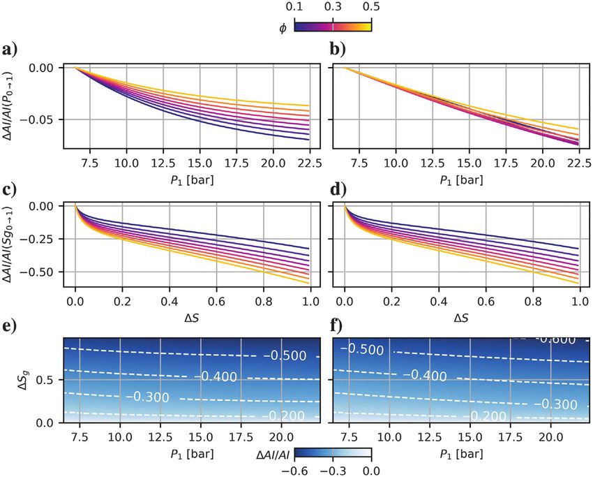
MR54                                                                      Weinzierl and Wiese

             tion of the shear-wave (S-wave) velocity. The nonlinear dependen-              (1980) to obtain a better fit for highly unconsolidated sediments
             cies between saturation, pressure, and seismic attributes require the          using a porosity-dependent Biot’s coefficient.
             application of rock-physics models, providing the means for a                     Pride et al. (1992) present explicit equations of motion as well
             discrimination between the different driving forces.                           as stress/strain relations in a dynamic two-phase porous medium
                The use of rock-physics models also allows us to consider site-             consisting of a fluid and matrix. Extending the work from Landrø
             specific data as prior knowledge by choosing an appropriate repre-             (2001), Lang and Grana (2019) present a Bayesian rock-physics
             sentation for the geologic conditions. The prior knowledge allows              inversion discriminating pore pressure and fluid effects. The two-
             us to shift the focus to the most relevant parameters in CO2 storage:          phase fluid distribution is frequently described by the Gassmann
             pressure, saturation, and porosity.                                            (1951) equation.
                A decrease in processing time, ideally in real time, increases the             Currently, there is a fast-growing application of deep neural net-
             operational value of the acquired data (Bertrand et al., 2014). By the         works to support interpretation and derive elastic properties from seis-
             application of machine-learning methods, the computational effort              mic data (Grana et al., 2017; Araya-Polo et al., 2018; Wu and Lin,
             can be reduced and a step toward faster evaluation can be made.                2018; Biswas et al., 2019; Das et al., 2019; Zheng et al., 2019;
                The presented methodology aims to support a planned near-sur-               Das and Mukerji, 2020). Applications of machine learning have
             face CO2 injection campaign, in which the seismic imaging is car-              long been constrained by limiting computational capacities. Now,
             ried out with a cross-well setup. The data sets in this study are              sufficiently large training data sets can be generated with forward mod-
             generated synthetically, with models and parameters adapted to a               eling to represent multiparameter moderate complex systems, which
             65 m deep unconsolidated glacial formation, located at the Svelvik             increases effort in the development of machine-learning approaches.
             ridge, Norway (Sørensen et al., 1990).                                         Gradient methods require numerically accurate forward models and
                Many potentially relevant rock-physics model formulations                   have problems in resolving discrete input data (Wiese et al., 2018).
             exist, but only some are applicable to the unconsolidated glacial              Deep neural networks do not show these disadvantages, and they
             deposits, with grain sizes from gravel to clay, that are present at the        are well suited to resolve the nonlinear dependencies between the pet-
             field site under investigation.                                                rophysical parameters and the corresponding elastic response (Raissi,
                The first soft-sand model was developed by Mindlin (1949). Biot             2018). Several recent studies have focused on full-waveform inversion
             (1956) then develops a theory including frequency-dependent con-               (FWI) in the context of deep convolutional neural networks (Mosser
             tributions for determining the poroelastic parameters. Raymer et al.           et al., 2018; Zhang and Stewart, 2019). Compared to traditional inver-
             (1980) propose a mixing approach to calculate poroelastic param-               sion, neural networks can provide a significant improvement in turn-
             eters for matrix and fluid phases that comprise more than one com-             around time. Xue et al. (2019) apply different machine-learning
             ponent. In this model, the poroelastic attributes compressional wave           techniques (e.g., neural networks and random forests) for mapping sat-
             (P-wave) velocity V P, S-wave velocity V S, and density ρ are func-            uration changes by analyzing normalized root-mean square amplitude
             tions of the porosity ϕ, clay volume V cl , and water saturation Sw .          changes and normalized differences of the reflection coefficient.
             Krief et al. (1990) further alter the relationships of Raymer et al.              In the present paper, deep neural networks are used as an inver-
                                                                                                                  sion tool to determine rock-physics properties
                                                                                                                  based on elastic attributes. Figure 1 shows the
                                                                                                                  flow scheme of the modeling approach. The
                                                                                                                  rock-physics parameters are the input to the
                                                                                                                  rock-physics forward model that is used to obtain
                                                                                                                  the poroelastic attributes. The training data set
                                                                                                                  comprising the rock-physics parameters and
                                                                                                                  resultant poroelastic attributes is then fed through
                                                                                                                  a sequence of increasingly deep neural networks.
                                                                                                                  Although the initial workload may be similar to a
                                                                                                                  conventional inversion, the human workload for
                                                                                                                  evaluating repeat surveys can be significantly re-
                                                                                                                  duced, as well as the time required for inversion.
                                                                                                                  This allows for near-real-time results and there-
                                                                                                                  fore improves the operational value of seismic
                                                                                                                  data (Moseley et al., 2018).
                                                                                                                     The poroelastic attributes V P , V S , ρ, QP , and QS
                                                                                                                  are taken as predetermined, either by inversion or
             Figure 1. Scheme of a three-layer neural network in prediction mode and the application              direct measurements from cross-well experiments,
             cases in this paper. The poroelastic attributes are at the left side, and the rock-physics           serving as observation data on which rock-physics
             parameters are at the right side. Note that, depending on the rock-physics model, only a
             subset of 3–5 poroelastic attributes is used. The V P , V S , and ρ are always input attrib-         parameters will be calibrated in a similar way as
             utes, and the dashed attributes are case dependent. The initial pressure P0 and depth z are          Xue et al. (2019). In the present paper, porosity
             not exactly rock-physics attributes, but they are on the input side because they are known           and pressure prior to injection are defined as addi-
             and affect the physics. Cases 1–3 comprise different rock-physics parameter sets as the              tional poroelastic attributes affecting the rock
             inversion target. These sets are simulated by different rock-physics models (indicated by
             the colored boxes). The structure of the paper follows the three steps of network selec-             physics. Saturation and pressure need to be explic-
             tion, feasibility, and reservoir application, in which the state of the art is consecutively         itly part of the rock-physics models to allow for
             enhanced by our developments.                                                                        their calibration. Because the consequences of

Downloaded from http://pubs.geoscienceworld.org/geophysics/article-pdf/doi/10.1190/geo2020-0049.1/5219751/geo-2020-0049.1.pdf
by GeoForschungsZentrums Potsdam user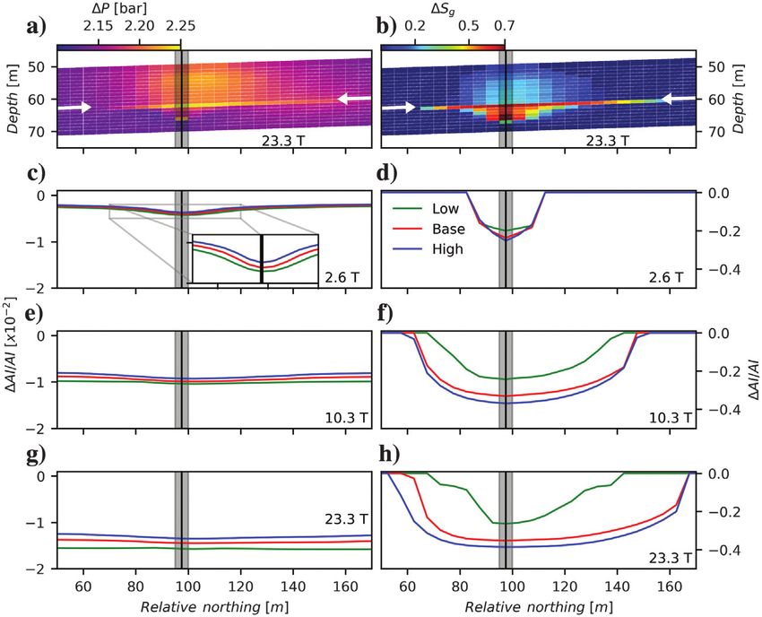
Deep learning a rock-physics model                                                                            MR55

                pressure variation effects on the poroelastic attributes are typically not                   Pressure dependence
                included in the rock-physics models, they are introduced into the ap-
                propriate formulations (Avseth et al., 2010; Lang and Grana, 2019).                             Neither rock-physics model (HMG and BG) includes a pressure
                   For field applications, the sensitivity of pressure dependence on                         dependence of the poroelastic attributes by definition. Therefore,
                the poroelastic attributes may be approximated from the attributes                           two independent pressure dependencies are introduced to both
                themselves but should ideally be carried out using direct measure-                           rock-physics models. According to Mavko and Mukerji (1998),
                ments from core plugs or well tests.                                                         the effective pressure Peff is the overburden pressure Pover minus
                   The current paper aims at methodological progress on two fields:                          the pore pressure Pp :
                first, the application of appropriate deep neural networks for seismic
                inversion; and second, the formulation and application of appropri-
                ate rock-physics models to distinguish pressure- and saturation-in-
                duced changes in seismic attributes.
                                                                                                                                        Peff ¼ Pover − Pp :                                 (2)

                                                 METHODS                                                     The pore pressure is further referred to as the baseline pressure P0
                Rock physics                                                                                 before (time T 0 ) and the monitor pressure P1 after (time T 1 ) injec-
                                                                                                             tion. An increase in the pore pressure results in a decrease of the
                    Two independent rock-physics models are used for forward mod-                            compressional forces acting at the grain contacts. As a consequence,
                eling the poroelastic attributes from rock-physics parameters. The first                     the velocity is decreased on the increased pore pressure, also called
                rock-physics model is called Hertz-Mindlin-Gassmann (HMG).                                   softening.
                It is based on the Hertz-Mindlin model in a soft-sand description (Min-                         The first velocity-pressure dependence follows Avseth et al.
                dlin, 1949). Although this model is strictly only valid for a single min-                    (2010), and it is referred to as PA:
                eral component, Hossain et al. (2011) show that this limitation can be
                overcome and demonstrate its applicability for two or more mineral
                components. In the current study, the matrix is a mixture of quartz
                                                                                                                                                         1 − aP;S · e−Peff;1 ∕Peff;0
                and clay and a perfectly patchy fluid distribution of the gas and water                                                                                        ~

                phase. The matrix and fluid phases are each described by a single ef-                                V P;S ðPeff;1 Þ ¼ V P;S ðPeff;0 Þ                                 ;    (3)
                                                                                                                                                         1 − aP;S · e−Peff;0 ∕Peff;0
                                                                                                                                                                               ~
                fective modulus (Domenico, 1977). The dry rock-physics parameters
                K d , Gd , and ρd are obtained by mixing the matrix components using
                the Hashin and Shtrikman (1963) bounds (also see Appendix A and
                Appendix B for variables not closely defined in the text).
                                                                                                             where V P;S refers to the P- and S-wave velocity and Peff;0;1 refers to
                    The rock-physics input parameters for HMG are the porosity ϕ,
                                                                                                             the effective baseline and monitor pressures. The scaling factors aP;S
                gas saturation Sg , pressure P, sand/clay mixing ratio (V cl ), bulk/
                                                                                                             are identical for both wave velocities and are kept constant at −0.2.
                shear modulus (K/G), and densities (ρ) of the frame and fluid phase.
                                                                                                             This value is within a realistic range for shallow unconsolidated sedi-
                The second rock-physics model is called Biot-Gassmann (BG), and
                                                                                                             ments, and the negative sign implies softening at the decreasing
                it is principally based on the poroelastic description introduced by
                                                                                                             effective pressure. An accurate pressure dependence is crucial,
                Biot (1956). The rock-physics input parameters are similar to the
                                                                                                             wherefore the scaling factors should ideally be determined for field
                HMG model. The dry moduli in the BG model are a function of
                                                                                                             conditions, for example, by core experiments or pumping tests. The
                the consolidation parameter cs. A higher consolidation factor in-
                                                                                                             term P~ eff;0 is a reference pressure, typically the maximal pressure.
                creases the matrix moduli in relation to the dry bulk moduli (equa-
                                                                                                                The second velocity-pressure dependency is based on the work of
                tions A-8 and A-9; Pride, 2005).
                                                                                                             Lang and Grana (2019), further referred to as pressure dependence
                    The fluid substitution in both models is described by the Gass-
                                                                                                             PL. Within this description, after defining ΔP ¼ P1 − P0 and for
                mann equation (Gassmann, 1951):
                                                                                                             the gas saturation ΔSg ¼ Sg1 − Sg0 , V P and V S are dependent on
                                K sat        Kd           K fl                                               ΔSg and ΔP showing a quadratic dependence on ϕ, whereas ρ
                                         ¼          þ                ;                           (1)         is only dependent on ϕ and ΔSg ,
                             K ma − K sat K ma − K d ϕðK ma − K fl Þ

                where K is the bulk modulus and the subscripts sat, ma, d, and fl
                denote saturated, matrix, dry, and fluid, respectively. For this paper,                         2              3
                                                                                                                  V P;1 ∕V P;0
                the rock-physics models are assumed to be calibrated. Although the
                                                                                                              ln4 V S;1 ∕V S;0 5
                Svelvik ridge consists of unconsolidated rock, the rock-physics
                                                                                                                    ρ1 ∕ρ0
                model BG describes consolidated rocks. Although this is not straight-                            2                                                        3
                forward and therefore prevents a direct application of the method to                               kα ðϕ;Sg ÞΔS2g þlα ðϕ;Sg ÞΔSg þmα ðϕ;PÞΔP2 þnα ðϕ;PÞΔP
                the Svelvik field site, this abstraction was carried out to demonstrate                        ¼ 4 kβ ðϕ;Sg ÞΔS2g þlβ ðϕ;Sg ÞΔSg þmβ ðϕ;PÞΔP2 þnβ ðϕ;PÞΔP 5;
                the applicability of the developed approach to real CO2 storage for-                                               kρ ðϕ;Sg ÞΔS2g þlρ ðϕ;Sg ÞΔSg
                mations, which are typically located in consolidated environments.                                                                                                          (4)
                   Due to their complexity, the equations are not presented here. The
                current implementation can be found in Appendix A; for a general
                overview, refer to Mavko et al. (2009).                                                      with

Downloaded from http://pubs.geoscienceworld.org/geophysics/article-pdf/doi/10.1190/geo2020-0049.1/5219751/geo-2020-0049.1.pdf
by GeoForschungsZentrums Potsdam user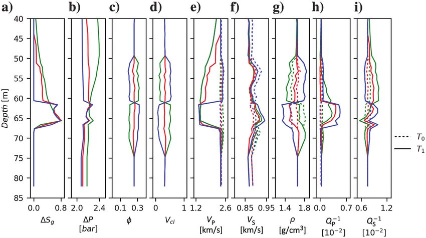
MR56 Weinzierl and Wiese
2 3
kα ðϕ; Sg Þ pressure-induced impedance change is strongly dependent on poros-
6 7 ity in PA but only slightly in PL. Further, PA shows a higher sensi-
6 lα ðϕ; Sg Þ 7
6 7 tivity to small pressure changes, which is less pronounced for PL.
6 m ðϕ; PÞ 7
4 α 5 For low porosities, the overall change in AI is similar, but for high
porosities, PL shows approximately 40% higher impedance changes.
nα ðϕ; PÞ
2 3 Because both pressure models rely on the Gassmann equation, the
a2 ðSg Þϕ2 þ a1 ðSg Þϕ þ a0 ; ai ¼ ai;1 Sg þ ai;0 impedance change due to saturation changes ΔS is identical for
6 7 both (Figure 2c and 2d). The velocity changes are highest for
6 b2 ðSg Þϕ2 þ b1 ðSg Þϕ þ b0 ; bi ¼ bi;1 Sg þ bi;0 7
¼6 6
7:
7
small gas saturations and become almost linear for saturations
4 c2 ðPÞϕ2 þ c1 ðPÞϕ þ c0 ; ci ¼ ci;1 P þ ci;0 5 >0.1. The lower row (Figure 2e and 2f) shows the ΔAI∕AI isolines
for pressure and saturation. In both pressure models, the isolines
d2 ðPÞϕ2 þ d1 ðPÞϕ þ d0 ; di ¼ di;1 P þ di;0
are roughly parallel, with the saturation effect far exceeding the pres-
(5) sure effect on the impedance. For the given ranges, a saturation
change has approximately a 10 times higher effect on the impedance
The relative acoustic impedance (AI) change between a monitor
than the pressure change with a higher pressure effect for PL
and baseline survey is determined according to Landro et al. (1999):
than for PA.
ΔAI V P;1 · ρ1 − V P;0 · ρ0
¼ : (6)
AI V P;0 · ρ0 Machine learning
A deep neural network acts as an inversion tool that derives rock-
Figure 2 shows the relative acoustic impedance change ΔAI∕AI for physics parameters plus pressure and saturation from poroelastic
different porosities caused by a pore pressure and saturation increase attributes. This is the reversed computation direction of the
with respect to the baseline conditions with P0 ¼ 6.5 bar and above-described rock-physics models. The neural network is
Sg;0 ¼ 0. Calculations are based on the HMG model with PA (Fig- trained with an ensemble. The training is performed with the po-
ure 2, the left column) and PL (Figure 2, the right column). The over- roelastic attributes as the network input and the rock-physics param-
all range of ΔAI∕AI is similar for both (Figure 2a and 2b). The eters as the expected network response.
Ensemble generation
For each learning case, one training ensemble
of size N T is generated. Such an ensemble con-
tains rock-physics parameters and the corre-
sponding forward-calculated poroelastic
attributes. The possible combinations of param-
eters and attributes are defined by the different
rock-physics model formulations, and the differ-
ent combinations used in the present work are
defined by the three cases (Figure 1). The
rock-physics parameters are generated with a
Monte Carlo approach; they are uniformly dis-
tributed within the parameter range and stochas-
tically independent. Depending on the rock-
physics inversion parameters, the remaining
parameters of the rock-physics forward model
are defaulted. This reduces the nonuniqueness
in the inversion and allows us to focus a priori
on the most unknown information. After rock-
physics simulation, inputs as well as the outputs
are scaled. The median is subtracted from the data,
which are then divided by the range between the
25 and 75 percentiles, such that the 25 and 75 per-
centiles are −1 and 1, respectively. For some
Figure 2. Acoustic impedance as a function of pressure and saturation. The left column generated rock-physics parameter sets, the corre-
corresponds to the pressure dependence in equation 3 (PA) and the right in Lang and sponding rock-physics model does not generate
Grana (2019) (PL). (a and b) The pressure dependence for 0.1 ≤ ϕ ≤ 0.5. The quadratic a solution. These sets are discarded and not in-
ϕ dependence in PL and the parameterization chosen for the unconsolidated environ- cluded in N T . Training is carried out with the en-
ment results in a crossover in the pressure curves for low porosities. Although it would
be possible to separate the pressure effect on the fluid and matrix phase, they are com- semble attributes as the input to the network and
bined in this site-specific description. The saturation component (c and d) is identical for the rock-physics parameters as the output to the
PA and PL. The total acoustic impedance change (e and f) is computed for ϕ ¼ 0.4. network.
Downloaded from http://pubs.geoscienceworld.org/geophysics/article-pdf/doi/10.1190/geo2020-0049.1/5219751/geo-2020-0049.1.pdf
by GeoForschungsZentrums Potsdam user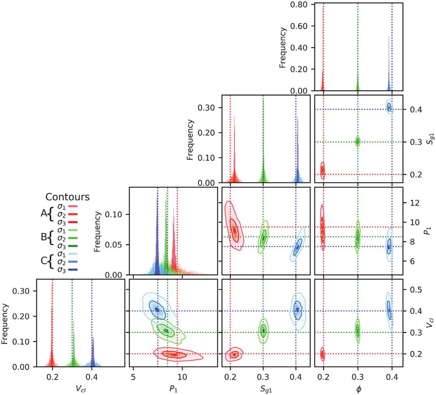
Deep learning a rock-physics model MR57
Network settings layer. Because there is no clear advantage in either of the approaches,
we continued computations with dropout decrease.
A suitable learning rate and weight decay are determined by grid
search and the AdamW optimizer (Kingma and Ba, 2014; Loshchilov
Validation
and Hutter, 2017). The values of 8 · 10−4 and 1.25 · 10−4 are used in
all following neural networks. The loss function can be interpreted as Accuracy (acc) is computed based on a validation ensemble,
an analog to an objective function in other inversion schemes. The L1 whose members are independent from the training ensemble:
smooth loss function is used as Girshick (2015) shows that the con-
vergence rate is increased by a factor of 3 to 10 compared to the PN V
i ðyi − mðxi ÞÞ
2
standard L1 (see equation 7). The L1 value has the form accðx; yÞ ¼ R2 ¼1− P NV
i ðyi − yÞ
2
1 X
N
X
V
NT
0.5ðxi − yi Þ2 ; if jxi − yi j < 1 with y ¼ y; (8)
L1 ¼ zi with zi ¼ ; (7) NV i i
i
jxi − yi j − 0.5; otherwise
with N V as the size of the validation ensemble.
with x as the training data and y as the predicted data. Activation is Based on the accuracy metric, early stopping is applied as an ad-
achieved by a rectified linear unit (ReLU) on the nodes (Nair and ditional measure to counteract overfitting (Prechelt, 1998). Similar
Hinton, 2010). Dropout was applied to prevent overfitting (Srivastava to a truncation criteria in traditional solver settings, further iteration
et al., 2014). A dropout decrease strategy was applied, with 30% stops. In the present approach, early stopping is applied after N S ¼
dropout on the first layer, decreasing by 10% for each successive 100 epochs after which no improvement of accuracy is achieved.
layer. The results are very similar to constant dropout of 30% for each
Table 1. Network configurations tested during the network- EXPERIMENTAL STRATEGY
selection step. The layer depth is between one and three, and
the number of neurons is between 100 and 2000 per layer. The experiments are carried out in three steps that build on one
another. The network size and structure with appropriate learning
rate are determined for an exemplary rock-physics model in the net-
Network no. No. of layers Configuration work selection step. The inversion feasibility is assessed for differ-
ent rock physical parameterizations under error-free conditions with
1 1 1000
a 0D model during the feasibility step. The approach is then applied
2 2 500 × 100 on a scenario-based simulation for a near-surface CO2 migration
3 2 1000 × 500 test in the reservoir application step.
4 3 1000 × 500 × 100
5 3 1000 × 1000 × 500 Network selection — Setup
6 3 1000 × 1000 × 1000 This step should find a suitable network configuration that shows
7 3 2000 × 2000 × 2000 fast learning and sufficient accuracy while avoiding overfitting. It is
not our aim to find the optimal network, which would require too
Table 2. Setup for the feasibility tests.
Case # Case 1 Case 2 Case 3
rock-physics model BG BG HMG
Pressure dependence — — PL
Range ½1 − A; 1 − B; 1 − C ½2 − A; 2 − B; 2 − C ½3 − A; 3 − B; 3 − C
ϕ [0.01, 0.99] [0.2, 0.3, 0.4] [0.2, 0.3, 0.4] [0.2, 0.3, 0.4]
K d ½GPa [1.0, 20.0] [7.0, 8.0, 9.0] 8.0 NA
Gd ½GPa [1.0, 20.0] [1.5, 2.0, 2.5] 2.0 NA
Sg [0.0, 1.0] 0.0 [0.2, 0.3, 0.4] [0.2, 0.3, 0.4]
P1 ½bar [6.5, 20.0] 6.5 6.5 [9.5, 8.5, 7.5]
cs [1.0, 10.0] 5.0 [4.0, 5.0, 6.0] NA
V cl [0.1, 0.7] NA NA [0.2, 0.3, 0.4]
Note: The range denotes rock-physics parameters for the ensemble generation. The values in brackets are the target values for inversion, and the other values are constant default
values. For each rock-physics reference value set, the poroelastic attributes are calculated. For example, case 1-B with ϕ 0.3, K d 8.0, Gd 2.0, Sg 0.0, P1 6.5, and cs 5.0. The V cl is not
included in feasibility.
Downloaded from http://pubs.geoscienceworld.org/geophysics/article-pdf/doi/10.1190/geo2020-0049.1/5219751/geo-2020-0049.1.pdf
by GeoForschungsZentrums Potsdam user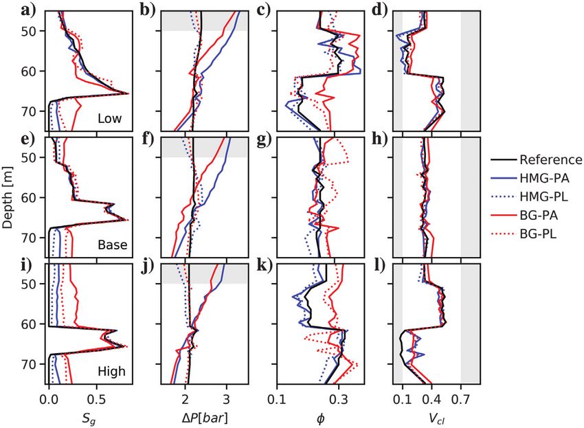
MR58                                                                      Weinzierl and Wiese

             much resources and, as conditions slightly change, would probably                            Feasibility tests — Setup
             not be optimal in the next steps.
                Seven network configurations with one to three layers and 600–                               Feasibility tests are carried out to assess the inversion power for
             6000 neurons are tested (Table 1). The training ensemble is gener-                           different rock-physics models and parameterizations. The selected
             ated with the BG rock-physics model for 0D and error-free condi-                             network #6 is applied to a training ensemble with 50,000 and a val-
             tions. The rock-physics parameters are ϕ, K d , and Gd , and the                             idation ensemble with 10,000 members.
             poroelastic attributes are V P , V S , and ρ. The training ensemble has                         Three formulations of the rock-physics models are tested in three
             50,000 members, and the validation ensemble has 10,000 members.                              0D cases. This allows us to evaluate the applicability of the developed
             The rock-physics parameters are generated in wide ranges to cover                            approach on different rock-physics problems for standard seismic
             all of the physically reasonable solution space (see the range in                            parameters (cases 1 and 2) and as well for one example of the devel-
             Table 2).                                                                                    oped rock-physics saturation and pressure discriminations (case 3). In
                                                                                                          a fully brine saturated medium, case 1 inverts for porosity ϕ and the
                                                                                                          dry frame moduli K d ; Gd . Case 2 inverts in a partially saturated
             Network selection — Results and discussion
                                                                                                          medium for porosity ϕ, gas saturation Sg , and the consolidation param-
                All networks show considerable learning. The loss functions are                           eter cs. Cases 1 and 2 are trained on the BG model (Table 2), analo-
             reduced by at least an order of magnitude, and the accuracy in-                              gous to conventionally inverted examples by Dupuy et al. (2016). Case
             creases by approximately two orders of magnitude (Figure 3).                                 3 is trained on the HMG model with pressure dependence PL.
             Deeper networks show a considerably faster loss reduction. Networks                             Each case is computed with two subcases: the first comprises
             #2 and #4, with the fewest number of neurons in the last layer, show                         P- and S-wave velocity and density (V P , V S , and ρ), and the second
             the least loss reduction, which can be partly attributed to the decrease                     comprises the latter plus attenuation attributes (QP and QS ). This
             of the dropout, which has a higher effect on lower layers. The final                         should determine the impact of the two attenuation attributes on
             accuracy ranges between 99.96% and 99.98%, which can be consid-                              inversion quality. Each of the six subcases is trained with an indi-
             ered very good in terms of fit. However small, a factor of two in                            vidual ensemble.
             the misfit remains. The dropout only affects the learning phase                                 For each case, three reference states are defined, named by letters
             and therefore the loss function, but during prediction all neurons                           A, B, and C, for example, case 1-B. For these reference states, the
             are used. The accuracy is therefore calculated including the dropout                         corresponding poroelastic attributes are inverted. The network is
             neurons, wherefore smaller shallower networks show good accuracy                             trained with an error-free ensemble. The statistical errors during de-
             values. Network #6 is chosen for further calculations because it                             termination of the poroelastic attributes are addressed by Monte
             shows the highest accuracy. Because dropout is affected by random-                           Carlo simulations during the inversion step. For each ensemble
             ness, the ranking is a snapshot because the loss and the accuracy in-                        member, an error realization is added to the reference set of poroe-
             clude a statistical component. An accurate interpretation would                              lastic attributes prior to inversion. Three error levels (σ 1;2;3 ) are de-
             require us to determine the statistical components characteristics.                          fined. They represent the accuracy for determining the poroelastic
             However, as described above, this is not the aim of the network se-                          attributes with different seismic acquisition methods and sub-
             lection step.                                                                                sequent inversion (see Table 3). Error 1 corresponds to a typical
                                                                                                          high-resolution surface seismic setup with errors in the range of
                                                                                                          100 m∕s for velocities (Table 4). Error 2 is realistic for an accurate
                                                                                                          vertical seismic profile (VSP) because the errors are reduced by a
                                                                                                          factor of two as a result of the increasing bandwidth in the range of
                                                                                                          8–400 Hz (Charles et al., 2019). Error 3 corresponds to cross-well
                                                                                                          acquisition, as planned for the Svelvik campaign. With a pick ac-
                                                                                                          curacy of two samples at a sampling rate of 0.03 ms, an accuracy of
                                                                                                          0.06 ms can be expected. This translates to an error band in veloc-
                                                                                                          ities of approximately 6 m∕s for a velocity of roughly 1700 m∕s.

                                                                                                          Table 3. Error levels for seismic acquisition.

                                                                                                          Var                             σ1                      σ2                       σ3

                                                                                                          V P [km/s]                   0.1                     0.05                     0.01
                                                                                                          V S [km/s]                   0.1                     0.05                     0.01
                                                                                                          ρ [g∕cm3 ]                   0.1                     0.05                     0.01
                                                                                                          Q−1
                                                                                                            P                          0.001                   0.0005                   0.0001
                                                                                                          Q−1
                                                                                                            S                          0.001                   0.0005                   0.0001

                                                                                                             Note: σ 1 corresponds to standard surface seismic, σ 2 corresponds to an accurate VSP
             Figure 3. Loss (solid, the left axis) and accuracy (dashed, the right                        setup, and σ 3 corresponds to an accurate cross-well setup. The errors are multiplied
             axis) of the feasibility test from the seven networks (Table 1), using                       with realizations from a 1 − σ windowed standard normal distribution and then
             early stopping with a stop set to 100 epochs.                                                added to the respective forward calculated poroelastic attribute.

Downloaded from http://pubs.geoscienceworld.org/geophysics/article-pdf/doi/10.1190/geo2020-0049.1/5219751/geo-2020-0049.1.pdf
by GeoForschungsZentrums Potsdam user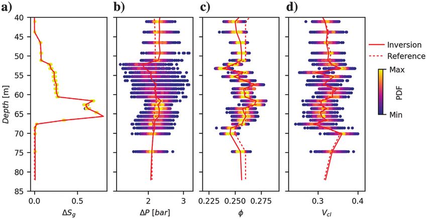
Table 4. Reference rock-physics parameters of cases 1–3 (denoted “True”) and the corresponding inversion results.
1-A 1-B 1-C
a) Case 1 ϕ Kd Gd ϕ Kd Gd ϕ Kd Gd
by GeoForschungsZentrums Potsdam user
True 0.2 7.0 1.5 0.3 8.0 2.0 0.4 9.0 2.5
Inverted Mean 0.22 7.21 1.77 0.30 8.06 2.33 0.39 9.12 2.88
f(V P ; V S ; ρ) Error bound 0.006 0.36 0.13 0.006 0.36 0.15 0.007 0.37 0.22
Inverted Mean 0.23 7.04 1.95 0.31 8.05 2.25 0.40 9.06 2.65
f(V P ; V S ; ρ, Error bound 0.003 0.23 0.07 0.004 0.28 0.13 0.005 0.36 0.18
QP ; QS )
b) Case 2 2-A 2-B 2-C
ϕ Sg cs ϕ Sg cs ϕ Sg cs
True 0.2 0.2 4.0 0.3 0.3 5.0 0.4 0.4 6.0
Inverted Mean 0.20 0.24 4.05 0.30 0.33 4.98 0.40 0.41 6.01
f(V P ; V S ; ρ) Error bound 0.005 0.03 0.14 0.005 0.04 0.18 0.006 0.03 0.22
Inverted Mean 0.21 0.22 3.96 0.31 0.31 4.95 0.40 0.40 5.99
f(V P ; V S ; ρ, Error bound 0.003 0.004 0.08 0.004 0.004 0.12 0.004 0.005 0.16
QP ; QS )
c) Case 3 3-A 3-B 3-C
ϕ Sg1 P1 V cl ϕ S1 P1 V cl ϕ Sg1 P1 V cl
True 0.2 0.2 9.5 0.2 0.3 0.3 8.5 0.3 0.4 0.4 7.5 0.4
Inverted Mean 0.20 0.21 9.30 0.19 0.30 0.31 8.46 0.30 0.40 0.40 7.62 0.40
Downloaded from http://pubs.geoscienceworld.org/geophysics/article-pdf/doi/10.1190/geo2020-0049.1/5219751/geo-2020-0049.1.pdf
f(V P ; V S ; ρ) Error bound 0.003 0.01 0.88 0.03 0.005 0.01 0.88 0.03 0.004 0.02 0.68 0.03
Inverted Mean 0.20 0.21 9.23 0.19 0.30 0.30 8.41 0.31 0.39 0.41 7.47 0.41
Deep learning a rock-physics model
f(V P ; V S ; ρ, Error bound 0.002 0.007 0.68 0.008 0.002 0.004 0.49 0.02 0.003 0.006 0.47 0.02
QP ; QS )
Note: The true sets of poroelastic parameters are overlain by a measurement error of a VSP seismic (σ 2 , Table 3). The error bounds reflect only this measurement error and include 90% of the realizations. Part (a) shows case 1, which is
rather a traditional setting inverting for porosity, bulk, and shear modulus in a fully saturated medium. Part (b) shows case 2, which inverts for porosity and, consolidation parameters as well as a saturation change. Part (c) shows case 3, which
inverts for porosity and, clay content as well as pressure and saturation changes.
MR59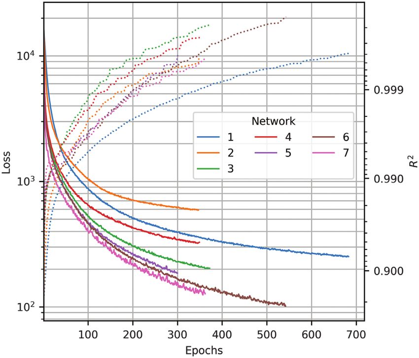
MR60 Weinzierl and Wiese
Feasibility tests — Results and discussion Gd , the inversion induces a systematic bias (or epistemic error) that
is larger than the aleatoric error that is induced by the seismic ac-
Table 4 summarizes the results of feasibility test cases 1–3, cal- quisition method. For case 2, ϕ and cs are determined very well
culated with error σ 2, corresponding to a VSP acquisition. For case (0%–5% deviation from the true value), with Sg showing an error
1, the mean of ϕ and K d is determined accurately (less than 5% of 0%–20%. With adding the attenuation parameters QP and QS , the
deviation), whereas Gd has errors of approximately 10%–15%. accuracy mostly increases and, most important, the largest error,
Adding QP and QS as inputs shows moderate improvements for the which is the error of Sg from case 2-A, is halved to 10%, which
deviation of the mean and also a reduction of the error bound, with we consider acceptable. The error bounds, that represent the meas-
the exception of Gd for reference parameters A, where the deviation urement error only, always decrease when attenuation parameters
of the mean increases from approximately 10% to 15%. For ϕ and are included. The deviation of the mean tends to improve with
the attenuation parameters included. However,
some deviation increases because the networks
with and without attenuation parameters are
trained with two different ensembles, respec-
tively. Further, the dropout is a stochastic effect
for each network, wherefore the models are not
perfect; that is, they have an epistemic uncer-
tainty and the results have a model-dependent
stochastic component. As an intermediate con-
clusion, the neural network shows a generally
good inversion capability for established rock-
physics models.
Therefore, the analyses continue with case 3 to
evaluate the applicability to invert for pressure
and saturation, which is the aim of this study.
The underlying rock-physics model for case 3
is HMG with the pressure dependence PL. Re-
sults are listed in Table 4c and are additionally
visualized in Figure 4. The mean of the inverted
rock-physics parameters deviates less than 5%
from the true values, which we consider very ac-
curate. Adding attenuation parameters has a de-
creasing effect on the pressure, causing a slight
increase of the misfit for case 3-A and 3-B, but a
slight decrease for case 3-C. Analogous to cases
1 and 2, including the attenuation parameters
decreases the error bounds. The calibration qual-
ity for all three cases is generally very good.
The error characteristics of the determined
Figure 4. Crossplot for case 3 of the feasibility test using attenuation as additional attrib-
utes. The terms σ 1 , σ 2 , and σ 3 refer to the errors of different seismic methods defined in rock-physics parameters are shown in Figure 4.
Table 3. Feasibility test on a separation of saturation and pressure in the HMG model and Crossplots of P1 show the largest error clouds,
pressure dependence PA with prediction results of the preferred network for case 3 using especially in relation to the saturation and the clay
V P ; V S ; and ρ for times T 0 and T 1 . The true values are visualized as a dashed crosshair content. The inversion for pressure would not be
below the diagonal and as a vertical line in the histograms along the diagonal. For de-
creasing errors σ 1 , σ 2 , and σ 3 , contours are drawn off-diagonal. meaningful with a surface seismic (corresponding
to error σ 1 ), but the area of the error cloud reduces
by approximately one order of magnitude with a
Table 5. Parameter settings for the three reservoir model VSP and two orders of magnitude for a cross-well seismic such that
scenarios. the inversion appears to be quite reliable with these methods.
The feasibility test shows that the neural network can determine
the rock-physics parameters generally with sufficient accuracy.
Cap rock Aquifer
Scenario Low Base High Low Base High RESERVOIR APPLICATION
Mϕ 1.2 1 0.8 0.8 1 1.2 Because the neural network has a demonstrated ability for dis-
Mκ 1.7 1 0.3 0.3 1 1.7 crimination of pressure and saturation in a 0D approach, it is evalu-
Pew ½bar 1 5 10 0.1 ated how it can be used for a field application. This is carried out
Peg ½bar 15 20 25 0.1 exemplarily at the Svelvik field site for CO2 storage, Norway (Wein-
zierl et al., 2018). Using both models (HMG and BG) each combined
Note: M ϕ and M κ are porosity and permeability multipliers, and Pew and Peg are with both pressure dependencies (PA and PL), four networks are
Brooks-Corey parameters for the two-phase flow behavior. trained.
Downloaded from http://pubs.geoscienceworld.org/geophysics/article-pdf/doi/10.1190/geo2020-0049.1/5219751/geo-2020-0049.1.pdf
by GeoForschungsZentrums Potsdam userDeep learning a rock-physics model MR61
Reservoir application — Setup and 5g). The differences for the low, base, and high case are small.
The total change of pressure-induced impedance is approximately
The Svelvik site is located on a glacial ridge with the subsurface 1.5% after 23 tons of injected CO2 . At the end of the injection,
consisting of glaciofluvial sand and gravel (Sørensen et al., 1990). A
the saturation-induced acoustic impedance ratio is approximately
glacial clay layer is present between 50 and 60 m that acts as cap
40% lower compared to the baseline. The saturation-induced imped-
rock to the reservoir (Hagby, 2018). The main properties affecting
ance ratio differs increasingly for the scenarios with increasing sim-
the sensitivity of the simulated injection plume extent are porosity
ulation time, mainly because of different amounts of CO2 migrating
and permeability. Formation velocities are known from the injection
into the cap rock.
well. Porosities are calculated on a Greenberg-
Castagna relation (Greenberg and Castagna,
1992). Permeabilities are derived from the poros-
ities using the Kozeny-Carman equation (Carman,
1961). To evaluate the applicability of the current
approach to different reservoir conditions and to
detect leakage, three scenarios are analyzed.
The base scenario represents the best prior
knowledge of the field site. For the low-contain-
ment scenario, the cap rock can be more easily
penetrated by CO2, by increasing porosity and
permeability, reducing the capillary entry pres-
sure. Additionally, a lower permeability of the
aquifer favors leakage. For the high scenario,
the reverse is done, with Brooks-Corey parame-
ters chosen such that no leakage occurs into
the cap rock. The scenarios are derived
with a multiplicator for the porosity (Mϕ ) and
permeability (Mκ ) (Table 5). For geologic consis-
tency, V cl is adjusted to the new porosities and
permeabilities for the high and low cases.
The capillary pressure Pc is defined by
−1∕λ
Sw − Swr
Pc ¼ Pe ; (9)
1 − Swr
Figure 5. Results of the reservoir model. (a and b) The pressure and saturation along a
with the capillary entry pressure Pe (Table 5), the north–south profile after the injection of 23 tons of CO2 for the base scenario. The im-
water saturation Sw , the residual water saturation pact of pressure and saturation on the acoustic impedance is visualized in (c-h) for in-
Swr ¼ 0.28, and the saturation exponent λ ¼ 3 creasing injection volumes in the highest reservoir layer, indicated by the white arrows in
(a and b). The low, base, and high scenarios are shown in colors green, red, and blue
constant for all scenarios. In total, 23 tons of lines, respectively. The black vertical line indicates the injection well.
CO2 are injected with a rate of 370 kg/d. The
outer boundary conditions are no-flow with a
pore volume multiplier on the outer cells. The
effective reservoir volume is 9.3 million cubic
meters (9.3 Mm3 ).
The reservoir model results are shown in Figure 5.
In all scenarios, the pressure buildup was slightly
higher than 2 bars, with the reservoir pressure in-
creasing by approximately 2.1 bars and an addi-
tional dynamic pressure increases of 0.15 bars in
the vicinity of the injection well (Figure 5a).
The CO2 saturation reaches values of 70%
close to the injection well, with lower values at
a larger distance. For the high scenario, no CO2
enters the cap rock, whereas for the low and base
scenarios, considerable concentrations of up to
27% are reached (Figure 5b).
The changes of the acoustic impedance are dis-
played separately for the impact of the pressure
Figure 6. From left to right: Four rock-physics input parameters and five forward-com-
and saturation changes (Figure 5). Because most puted poroelastic attributes calculated with the HMG model and pressure dependence
of the pressure buildup is static, the impedance PL along the injection well after 23 tons of injected CO2 . If a dashed line is present, it
ratio shows a rather flat profile (Figure 5c, 5e, refers to the situation before CO2 injection.
Downloaded from http://pubs.geoscienceworld.org/geophysics/article-pdf/doi/10.1190/geo2020-0049.1/5219751/geo-2020-0049.1.pdf
by GeoForschungsZentrums Potsdam userMR62 Weinzierl and Wiese
Four individual networks for both rock-physics models (HMG and the HMG model. Saturation is also generally inverted quite accu-
BG) each combined with both pressure dependencies (PA and PL) are rately. The highest deviations occur for regions without CO2 satu-
trained with the hydrostatic initial pressure as P0 . The networks are ration with differences of three saturation percentage points for the
trained with an ensemble of 200,000 members. The reservoir model BG model in combination with the Avseth pressure dependency.
training phase (as the largest model) was finished in approximately 1 h The deviation is highest above the reservoir, apparently correlated
on a GeForce GTX 1070. The prediction for 100 K configurations can to the lower reference porosity.
be performed in less than 2 s. The pressure changes are very accurate for PL, whereas PA
shows very good values only in the reservoir. Above the pressure
Reservoir application — Results and discussion is underestimated and below overestimated by up to 0.8 bars, ap-
parently mainly affected by the depth and therefore by the hydro-
The inversion capability is demonstrated at the injection well lo-
static pore pressure. The lowest pressures of the training ensembles
cation because the saturation and pressure contrasts are the highest
are 5 bar, wherefore greater than 50 m the pressure model is unde-
here. In the case of real-world application, the local poroelastic
fined. Nevertheless, this hardly affects the models. PL does not
attributes at the Svelvik#2 injection well can be determined by
show an extra error here because the pressure difference is consid-
2D seismic inversion due to the cross-well setup.
ered, whereas PA is implemented based on the difference of the
The output from the reservoir model, geologic model, and the
absolute values. Although PL is based on absolute pressures, the
poroelastic attributes forward modeled with the HMG-PL model is
additional deviation outside the training interval is marginal. For the
shown in Figure 6. The rock-physics parameters from the reservoir
clay content, the training range has a more pronounced effect. For
simulation are ΔSg , ΔP, and the geologically derived parameters ϕ
the clay content approaching the training boundary of 0.1, as be-
and V cl . The attribute V p is strongly affected by saturation, whereas
V s is more affected by the porosity and the pressure. Similarly, Qp tween 50 and 60 m for the low-containment scenario, the error ap-
is more affected by saturation and Qs more by pressure. The density pears to be slightly higher compared to other depths. The effect is
ρ is mainly affected by the clay content, but also by the saturation. stronger and results in an overestimation when the clay content is
The inversion results of saturation, porosity, and clay content are slightly lower than the training range as between 60 and 70 m for
quite close to the reference truth for most scenarios and rock-phys- the high-containment scenario. All inversion results are satisfying,
ics models. Therefore, the misfit is 10 times exaggerated for ϕ, Sg , with the best results obtained for the HMG-PL model.
and V cl to allow for a better interpretation, but ΔP predictions are The HMG model shows very good prediction quality because it
not exaggerated because they have a higher deviation (Figure 7). refers to unconsolidated rocks. However, although the BG model is
Porosity is inverted quite accurately, with slight advantages for developed for consolidated environments, it shows satisfying re-
sults. Therefore, this approach is also applicable
to CO2 storage formations, which are located in
deep consolidated formations. A comparison
under CO2 conditions probably would show ad-
vantages for the BG model.
All simulations are calculated with individual
ensembles and individual seeds for dropout,
wherefore the analysis includes epistemic errors
(errors that refer to the inversion method). Never-
theless, these errors are apparently smaller than
the systematic deviations of the methods.
The effect of the measurement error (also re-
ferred as aleatoric error) on the inversion quality
is exemplarily analyzed with the HMG-PL model
for the base case. The measurement error of an
accurate cross-well seismic is applied (σ 3 , Ta-
ble 3). The inversion for saturation is most reli-
able. In the reservoir and other regions where
CO2 is present, there is a variation width of typ-
ically approximately 2%−3% in saturation,
with a maximum of almost 5% in the reservoir,
where the highest saturations are present (Fig-
ure 8). However, the simulated saturations of
greater than 50%, at which the highest bandwidth
Figure 7. Error-free predictions for different rock-physics formulations. HMG and BG occurs, might be higher than found in the field.
are each combined with pressure dependence PA (Avseth et al., 2010) and PL (Lang and The error band of the pressure is approxi-
Grana, 2019). The rows from top to bottom show the low-, base-, and high-containment mately 0.7 bar for regions where CO2 is
scenarios after injection of 23 tons of CO2 . The black line is the synthetic truth, and it is present, which is a mediocre accuracy compared
referred to by the x-axis. The colored lines show the misfit of the predictions in 10 fold
exaggeration, and only for the pressure difference the misfit is not exaggerated. The to traditional pressure measurements. Never-
shaded areas in the pressure and clay content columns are outside the parameter range theless, it is considerably lower than the pressure
of the ensembles. variation itself and therefore might provide valu-
Downloaded from http://pubs.geoscienceworld.org/geophysics/article-pdf/doi/10.1190/geo2020-0049.1/5219751/geo-2020-0049.1.pdf
by GeoForschungsZentrums Potsdam userDeep learning a rock-physics model MR63
based on the HMG equations, and the second
is a hard rock formulation based on the BG equa-
tions. Although the HMG and BG equations con-
sider different physical processes, their forward
and also inverse behavior is similar for the cur-
rent parameterization, with the HMG model
showing a slightly better behavior for the ana-
lyzed field example of the shallow Svelvik aqui-
fer. The BG model is more promising for the
intended real-world CO2 storage application in
deeper and consolidated formations.
It is recommended to include as many poroe-
lastic attributes as possible; including P- and S-
wave attenuation, the accuracy tends to increase.
Pressure inversion provides meaningful results.
Figure 8. Impact of measurement error on the prediction accuracy with the HMG-PL However, the accuracy of determining the pres-
model at the injection well location after injection of 23 tons of CO2 for the base sce- sure is still lower compared with the other rock-
nario. Stochastic realizations are based on measurement error σ 3 (Table 3), valid for an physics parameters. Differential analysis, includ-
accurate cross-well seismic. The dashed line is the reference values, and the solid line is ing baseline data acquired without subsurface gas
the error-free inversion. The color refers to the density of the realizations relative to
equal distribution over the respective x-axis. Max indicates a sixfold higher density com- saturation, is a prerequisite for pressure and sat-
pared to the equal distribution, and min a sixth in the density. White indicates no real- uration discrimination. The method appears
izations. The depths follow the reservoir discretization. promising for gas storage and other applications,
as long as the gas content of the baseline is zero
such that many of the unknown errors cancel out.
able information for regions with low pressure gauge coverage. Compared to the traditional AVO-based methods, the rock-physics
Above the reservoir, however, the error bound grows to 1 bar. approach is a significant advance in the determination of pressure
Further, the values are more equally distributed and have a smaller from poroelastic attributes.
centric tendency. It is remarkable to distinguish the pressure with Many assumptions have to be made in developing a site-specific
such accuracy because the seismic impedance varies by 40% for rock-physics description of the subsurface. For the current study, the
saturations and only by 1.5% for pressure. With the deep neural favorable assumption of an intermediate patchy gas distribution in the
network, it is possible to take advantage of the nonlinear effects subsurface is made. Under the conditions of a known intermediate-
on the different poroelastic attributes. The error bounds of the patchy gas distribution, the epistemic error, that is, the error of the
porosity are approximately 2%, with a pronounced central ten- inversion algorithm itself, is smaller than the conceptual error of the
dency, which is considered quite accurate. The clay content has rock physics. The latter is smaller than the aleatoric error, that is, the
larger error bounds of 5%. measurement error for an accurate cross-well seismic. For real-world
However, it has to be considered that the current analysis is re- applications, a sufficiently patchy gas distribution is a prerequisite.
stricted to a subset of possible parameters. Under real-world con- The developed neural network was found applicable for inverting
ditions, a null space of different inversion results with equal quality the rock-physics equations. Although the quality of neural network
of fit to the data would occur. A promising development is the recent results may vary under different conditions, we see great potential to
advance in FWI techniques. They are also based on deep convolu- replace traditional inversion tools, especially if the bandwidth of the
tional networks, use the full-wavefield information; therefore, they expected results is known, as is the case in gas storage applications.
allow us to invert for high-resolution velocities. We think that their For industry application, the rapid results after the monitoring cam-
combination with our approach has the potential for providing suf- paigns are a significant advantage to traditional inversion, allowing
ficiently accurate poroelastic attributes that allow discrimination of a faster reaction to unforeseen events.
pressure and saturation. An accurate determination of the poroelastic attributes is the cur-
In this paper, the synthetic truth itself is generated by a rock- rent bottleneck of the method. Recent FWI techniques, also based
physics model. In the real world, the rock may show differences on deep convolutional networks, use the full-wavefield information
from the rock-physics model formulation. This is particularly im- and therefore allow us to invert for high-resolution velocities. We
portant because for the current study the favorable assumption of an think that their combination with our approach has the potential for
intermediate patchy gas distribution in the subsurface is made. The a much better discrimination of pressure and saturation. The devel-
variation to more homogeneous gas distribution would increase the oped methodology may then be used to derive high-resolution
nonlinearity and, therefore, the error of the current method (Eid petrophysical properties.
et al., 2015). Even more important is the difficulty in correctly
defining an effective patchiness.
ACKNOWLEDGMENTS
CONCLUSION This work has been produced with support from the Pre-ACT
project (project no. 271497) funded by RCN (Norway), Gassnova
Two rock-physics models are developed that allow us to discrimi- (Norway), BEIS (UK), RVO (Netherlands), and BMWi (Germany)
nate pressure and saturation. The first is a soft-sand formulation and cofunded by the European Commission under the Horizon
Downloaded from http://pubs.geoscienceworld.org/geophysics/article-pdf/doi/10.1190/geo2020-0049.1/5219751/geo-2020-0049.1.pdf
by GeoForschungsZentrums Potsdam userMR64 Weinzierl and Wiese
2020 programme, ACT grant agreement no. 691712. We also ac- As a simplified approach, the dry moduli are calibrated with pressure
knowledge the industry partners for their contributions: Total, Equi- P equal to the injection location at 65 m depth at 6.5 bar. It would be
nor, Shell, and TAQA. We would like to thank the editor in chief J. more accurate to calibrate each zone or formation at its depth.
Shragge and assistant editor E. Gasperikova as well as the three The second rock-physics model is the BG model, outlined in de-
anonymous reviewers for the many constructive comments. tail in Pride et al. (2004). The dry bulk and shear moduli of the rock-
physics model are dependent on a consolidation parameter (cs) and
are defined by
DATA AND MATERIALS AVAILABILITY
1−ϕ
Data associated with this research are available and can be ½BG∶K d ¼ K ma ; (A-8)
1 þ csϕ
obtained by contacting the corresponding author.
1−ϕ
½BG∶Gd ¼ Gma : (A-9)
APPENDIX A 1 þ 32 csϕ
DESCRIPTION OF ROCK-PHYSICS MODELS
Solid and fluid mixing
Dry moduli The density of the subsurface is calculated as the matrix density
The first rock-physics model is the Hertz-Mindlin soft-sand and fluid density filling the pore space:
model (HMG), in which the Gassmann equation (see equation 1)
determines the bulk and shear moduli of the saturated and dry rock ρ ¼ ϕρfl þ ð1 − ϕÞρma : (A-10)
based on the porosity ϕ and fluid modulus:
We consider a mixture of quartz (K 1 ; G1 ) and clay (K 2 ; G2 ) with the
−1 corresponding volume fractions (f 1 ¼ ð1 − V cl Þ; f 2 ¼ V cl ). For
ϕ∕ϕC 1−ϕ∕ϕC 4
½HMG∶K d ¼ þ − GHM ; averaging, we choose the Hashin-Shtrikman method with the upper
K HM þ4GHM ∕3 K HM þ4GHM ∕3 3
and lower bounds obtained by interchanging subscripts 1 and 2,
(A-1) respectively:
f2
K HS ¼ K 1 þ −1
(A-11)
−1 ðK 2 − K 1 Þ þ f 1 ðK 1 þ 4G1 ∕3Þ−1
ϕ∕ϕC 1 − ϕ∕ϕC
½HMG∶Gd ¼ þ −z (A-2)
GHM þ z GHM þ z
GHS ¼G1
with f2
þ :
GHM 9K HM þ 8GHM ðG2 −G1 Þ−1 þ2f 1 ðK 1 þ2G1 Þ∕½5G1 ðK 1 þ4G1 ∕3Þ
z¼ : (A-3) (A-12)
6 K HM þ 2GHM
In our case, matrix constituents are mixed with Sm ¼ 0.5 yielding the
For the critical porosity and coordination number, the standard val-
arithmetic average of the lower and upper Hashin-Shtrikman bounds:
ues of ϕc ¼ 0.4 and n ¼ 8.6 are used. The coordination number n is
obtained from the Murphy (1982) empirical relation with ϕ ¼ ϕc ,
K ma ¼ Sm K HSþ þ ð1 − Sm ÞK HS− : (A-13)
n ¼ 20 − 34ϕ þ 14ϕ2 ; (A-4) For both models, fluid mixing is achieved according to (Brie et al.,
1995):
as outlined in Avseth et al. (2010). The bulk and shear modulus
(K HM and GHM ) of the Hertz-Mindlin moduli are defined as ½BG∕HMG∶K fl ¼ ðK w − K g Þð1 − Sg Þe þ K g ; (A-14)
n2 ð1 − ϕc Þ2 G2 1∕3 with the exponent set fixed to e ¼ 5.
K HM ¼ P ; (A-5)
18π 2 ð1 − νÞ
Viscoelasticity
The velocity and attenuation are calculated based on the bulk modu-
1∕3 lus K fl , density ρfl, and viscosity η. The complex permeability κðωÞ
5 − 4ν 3n2 ð1 − ϕc Þ2 G2 is dependent on the permeability κ 0 and the angular frequency ω:
GHM ¼ P (A-6)
5ð2 − νÞ 2π ð1 − νÞ
2
κ0
κðωÞ ¼ qffiffiffiffiffiffiffiffiffiffiffiffiffiffiffiffiffi ; (A-15)
with the shear Poisson’s ratio ν as 1 − 12 i ωωc − i ωωc
3K ma − 2Gma
ν¼ : (A-7) with κ 0 ¼ 10−12 ½m2 being fixed. The angular frequency ωc is de-
2ð3K ma þ Gma Þ fined as
Downloaded from http://pubs.geoscienceworld.org/geophysics/article-pdf/doi/10.1190/geo2020-0049.1/5219751/geo-2020-0049.1.pdf
by GeoForschungsZentrums Potsdam userYou can also read