RainNet v1.0: a convolutional neural network for radar-based precipitation nowcasting
←
→
Page content transcription
If your browser does not render page correctly, please read the page content below
Geosci. Model Dev., 13, 2631–2644, 2020
https://doi.org/10.5194/gmd-13-2631-2020
© Author(s) 2020. This work is distributed under
the Creative Commons Attribution 4.0 License.

RainNet v1.0: a convolutional neural network for
radar-based precipitation nowcasting
Georgy Ayzel1 , Tobias Scheffer2 , and Maik Heistermann1
1 Institute   for Environmental Sciences and Geography, University of Potsdam, Potsdam, Germany
2 Department      of Computer Science, University of Potsdam, Potsdam, Germany

Correspondence: Georgy Ayzel (ayzel@uni-potsdam.de)

Received: 30 January 2020 – Discussion started: 4 March 2020
Revised: 7 May 2020 – Accepted: 13 May 2020 – Published: 11 June 2020

Abstract. In this study, we present RainNet, a deep convo-         length scales of 16 km and below. Obviously, RainNet had
lutional neural network for radar-based precipitation now-         learned an optimal level of smoothing to produce a nowcast
casting. Its design was inspired by the U-Net and SegNet           at 5 min lead time. In that sense, the loss of spectral power
families of deep learning models, which were originally de-        at small scales is informative, too, as it reflects the limits of
signed for binary segmentation tasks. RainNet was trained          predictability as a function of spatial scale. Beyond the lead
to predict continuous precipitation intensities at a lead time     time of 5 min, however, the increasing level of smoothing is
of 5 min, using several years of quality-controlled weather        a mere artifact – an analogue to numerical diffusion – that
radar composites provided by the German Weather Service            is not a property of RainNet itself but of its recursive ap-
(DWD). That data set covers Germany with a spatial do-             plication. In the context of early warning, the smoothing is
main of 900 km × 900 km and has a resolution of 1 km in            particularly unfavorable since pronounced features of intense
space and 5 min in time. Independent verification experi-          precipitation tend to get lost over longer lead times. Hence,
ments were carried out on 11 summer precipitation events           we propose several options to address this issue in prospec-
from 2016 to 2017. In order to achieve a lead time of 1 h,         tive research, including an adjustment of the loss function
a recursive approach was implemented by using RainNet pre-         for model training, model training for longer lead times, and
dictions at 5 min lead times as model inputs for longer lead       the prediction of threshold exceedance in terms of a binary
times. In the verification experiments, trivial Eulerian persis-   segmentation task. Furthermore, we suggest additional in-
tence and a conventional model based on optical flow served        put data that could help to better identify situations with im-
as benchmarks. The latter is available in the rainymotion li-      minent precipitation dynamics. The model code, pretrained
brary and had previously been shown to outperform DWD’s            weights, and training data are provided in open repositories
operational nowcasting model for the same set of verification      as an input for such future studies.
events.
   RainNet significantly outperforms the benchmark models
at all lead times up to 60 min for the routine verification met-
rics mean absolute error (MAE) and the critical success in-        1   Introduction
dex (CSI) at intensity thresholds of 0.125, 1, and 5 mm h−1 .
However, rainymotion turned out to be superior in predicting       The term “nowcasting” refers to forecasts of precipitation
the exceedance of higher intensity thresholds (here 10 and         field movement and evolution at high spatiotemporal reso-
15 mm h−1 ). The limited ability of RainNet to predict heavy       lutions (1–10 min, 100–1000 m) and short lead times (min-
rainfall intensities is an undesirable property which we at-       utes to a few hours). Nowcasts have become popular not
tribute to a high level of spatial smoothing introduced by the     only with a broad civil community for planning everyday ac-
model. At a lead time of 5 min, an analysis of power spec-         tivities; they are particularly relevant as part of early warn-
tral density confirmed a significant loss of spectral power at     ing systems for heavy rainfall and related impacts such as
                                                                   flash floods or landslides. While the recent advances in high-

Published by Copernicus Publications on behalf of the European Geosciences Union.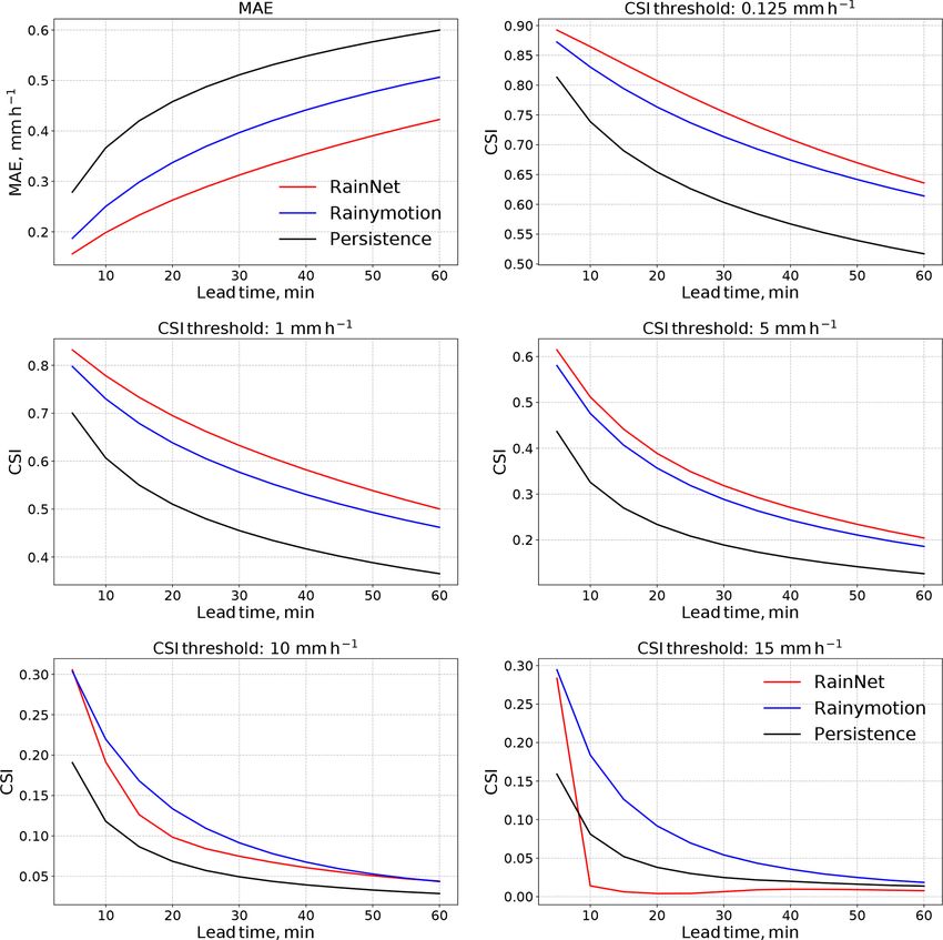
2632                                  G. Ayzel et al.: RainNet: a convolutional neural network for precipitation nowcasting

performance computing and data assimilation significantly           tion nowcasting is still in its infancy, and universal solutions
improved numerical weather prediction (NWP) (Bauer et al.,          are not yet available. Shi et al. (2015) were the first to in-
2015), the computational resources required to forecast pre-        troduce deep learning models in the field of radar-based pre-
cipitation field dynamics at very high spatial and temporal         cipitation nowcasting: they presented a convolutional long
resolutions are typically prohibitive for the frequent update       short-term memory (ConvLSTM) architecture, which out-
cycles (5–10 min) that are required for operational nowcast-        performed the optical-flow-based ROVER (Real-time Opti-
ing systems. Furthermore, the heuristic extrapolation of pre-       cal flow by Variational methods for Echoes of Radar) now-
cipitation dynamics that are observed by weather radars still       casting system in the Hong Kong area. A follow-up study
outperforms NWP forecasts at short lead times (Lin et al.,          (Shi et al., 2017) introduced new deep learning architectures,
2005; Sun et al., 2014). Thus, the development of new now-          namely the trajectory gated recurrent unit (TrajGRU) and the
casting systems based on parsimonious but reliable and fast         convolutional gated recurrent unit (ConvGRU), and demon-
techniques remains an essential trait in both atmospheric and       strated that these models outperform the ROVER nowcasting
natural hazard research.                                            system, too. Further studies by Singh et al. (2017) and Shi
   There are many nowcasting systems which work opera-              et al. (2018) confirmed the potential of deep learning models
tionally all around the world to provide precipitation now-         for radar-based precipitation nowcasting for different sites in
casts (Reyniers, 2008; Wilson et al., 1998). These systems,         the US and China. Most recently, Agrawal et al. (2019) in-
at their core, utilize a two-step procedure that was originally     troduced a U-Net-based deep learning model for the predic-
suggested by Austin and Bellon (1974), consisting of track-         tion of the exceedance of specific rainfall intensity thresholds
ing and extrapolation. In the tracking step, a velocity is ob-      compared to optical flow and numerical weather prediction
tained from a series of consecutive radar images. In the ex-        models. Hence, the exploration of deep learning techniques
trapolation step, that velocity is used to propagate the most       in radar-based nowcasting has begun, and the potential to
recent precipitation observation into the future. Various fla-      overcome the limitations of standard tracking and extrapola-
vors and variations of this fundamental idea have been de-          tion techniques has become apparent. There is a strong need,
veloped and operationalized over the past decades, which            though, to further investigate different architectures, to set up
provide value to users of corresponding products. Still, the        new benchmark experiments, and to understand under which
fundamental approach to nowcasting has not changed much             conditions deep learning models can be a viable option for
over recent years – a situation that might change with the          operational services.
increasing popularity of deep learning in various scientific           In this paper, we introduce RainNet – a deep neural net-
disciplines.                                                        work which aims at learning representations of spatiotempo-
   “Deep learning” refers to machine-learning methods for           ral precipitation field movement and evolution from a mas-
artificial neural networks with “deep” architectures. Rather        sive, open radar data archive to provide skillful precipitation
than relying on engineered features, deep learning derives          nowcasts. The present study outlines RainNet’s architecture
low-level image features on the lowest layers of a hierarchi-       and its training and reports on a set of benchmark exper-
cal network and increasingly abstract features on the high-         iments in which RainNet competes against a conventional
level network layers as part of the solution of an optimization     nowcasting model based on optical flow. Based on these ex-
problem based on training data (LeCun et al., 2015). Deep           periments, we evaluate the potential of RainNet for now-
learning began its rise from the field of computer science          casting but also its limitations in comparison to conventional
when it started to dramatically outperform reference methods        radar-based nowcasting techniques. Based on this evaluation,
in image classification (Krizhevsky et al., 2012) and machine       we attempt to highlight options for future research towards
translation (Sutskever et al., 2014), which was followed by         the application of deep learning in the field of precipitation
speech recognition (LeCun et al., 2015). Three main reasons         nowcasting.
caused this substantial breakthrough in predictive efficacy:
the availability of “big data” for model training, the develop-
ment of activation functions and network architectures that         2     Model description
result in numerically stable gradients across many network
layers (Dahl et al., 2013), and the ability to scale the learning   2.1    Network architecture
process massively through parallelization on graphics pro-
cessing units (GPUs). Today, deep learning is rapidly spread-       To investigate the potential of deep neural networks for radar-
ing into many data-rich scientific disciplines, and it comple-      based precipitation nowcasting, we developed RainNet –
ments researchers’ toolboxes with efficient predictive mod-         a convolutional deep neural network (Fig. 1). Its architec-
els, including in the field of geosciences (Reichstein et al.,      ture was inspired by the U-Net and SegNet families of deep
2019).                                                              learning models for binary segmentation (Badrinarayanan
   While expectations in the atmospheric sciences are high          et al., 2017; Ronneberger et al., 2015; Iglovikov and Shvets,
(see, e.g., Dueben and Bauer, 2018; Gentine et al., 2018),          2018). These models follow an encoder–decoder architecture
the investigation of deep learning in radar-based precipita-        in which the encoder progressively downscales the spatial

Geosci. Model Dev., 13, 2631–2644, 2020                                              https://doi.org/10.5194/gmd-13-2631-2020

G. Ayzel et al.: RainNet: a convolutional neural network for precipitation nowcasting                                                2633

Figure 1. Illustration of the RainNet architecture. RainNet is a convolutional deep neural network which follows a standard encoder–decoder
structure with skip connections between its branches. See main text for further explanation.

resolution using pooling, followed by convolutional layers,             put volume with a step-size parameter (or stride; stride = 1 in
and the decoder progressively upscales the learned patterns             this study) and produces a dot product between filter weights
to a higher spatial resolution using upsampling, followed by            and corresponding input volume values. A bias parameter is
convolutional layers. There are skip connections (Srivastava            added to this dot product, and the results are transformed us-
et al., 2015) from the encoder to the decoder in order to en-           ing an adequate activation function. The purpose of the ac-
sure semantic connectivity between features on different lay-           tivation function is to add nonlinearities to the convolutional
ers.                                                                    layer output – to enrich it to learn nonlinear features. To in-
   As elementary building blocks, RainNet has 20 convolu-               crease the efficiency of convolutional layers, it is necessary
tional, 4 max pooling, 4 upsampling, and 2 dropout layers               to optimize their hyperparameters (such as number of filters,
and 4 skip connections. Convolutional layers aim to gener-              kernel size, and type of activation function). This has been
ate data-driven spatial features from the corresponding in-             done in a heuristic tuning procedure (not shown). As a result,
put volume using several convolutional filters. Each filter is          we use convolutional layers with up to 1024 filters, kernel
a three-dimensional tensor of learnable weights with a small            sizes of 1 × 1 and 3 × 3, and linear or rectified linear unit
spatial kernel size (e.g., 3 × 3, and the third dimension equal         (ReLU; Nair and Hinton, 2010) activation functions.
to that of the input volume). A filter convolves through the in-

https://doi.org/10.5194/gmd-13-2631-2020                                                   Geosci. Model Dev., 13, 2631–2644, 2020
2634 G. Ayzel et al.: RainNet: a convolutional neural network for precipitation nowcasting
Using a max pooling layer has two primary reasons: it RainNet differs fundamentally from ConvLSTM (Shi
achieves an invariance to scale transformations of detected et al., 2015), a prior neural-network approach, which ac-
features and increases the network’s robustness to noise and counts for both spatial and temporal structures in radar data
clutter (Boureau et al., 2010). The filter of a max pooling by using stacked convolutional and long short-term memory
layer slides over the input volume independently for every (LSTM) layers that preserve the spatial resolution of the in-
feature map with some step parameter (or stride) and resizes put data alongside all the computational layers. LSTM net-
it spatially using the maximum (max) operator. In our study, works have been observed to be brittle; in several application
each max pooling layer filter is 2 × 2 in size, applied with domains, convolutional neural networks have turned out to be
a stride of 2. Thus, we take the maximum of four numbers in numerically more stable during training and make more ac-
the filter region (2 × 2), which downsamples our input vol- curate predictions than these recurrent neural networks (e.g.,
ume by a factor of 2. In contrast to a max pooling layer, an Bai et al., 2018; Gehring et al., 2017).
upsampling layer is designed for the spatial upsampling of Therefore, RainNet uses a fully convolutional architec-
the input volume (Long et al., 2015). An upsampling layer ture and does not use LSTM layers to propagate information
operator slides over the input volume and fills (copies) each through time. In order to make predictions with a larger lead
input value to a region that is defined by the upsampling ker- time, we apply RainNet recursively. After predicting the es-
nel size (2 × 2 in this study). timated log precipitation for t + 5 min, the measured values
Skip connections were proposed by Srivastava et al. (2015) for t −10, t −5, and t, as well as the estimated value for t +5,
in order to avoid the problem of vanishing gradients for the serve as the next input volume which yields the estimated log
training of very deep neural networks. Today, skip connec- precipitation for t +10 min. The input window is then moved
tions are a standard group of methods for any form of infor- on incrementally.
mation transfer between different layers in a neural network
(Gu et al., 2018). They allow for the most common patterns 2.2 Optimization procedure
learned on the bottom layers to be reused by the top layers in
order to maintain a connection between different data repre- In total, RainNet has almost 31.4 million parameters. We
sentations along the whole network. Skip connections turned optimized these parameters using a procedure of which we
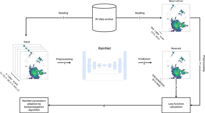
out to be crucial for deep neural network efficiency in recent show one iteration in Fig. 2: first, we read a sample of in-
studies (Iglovikov and Shvets, 2018). For RainNet, we use put data that consists of radar composite grids at time t − 15,
skip connections for the transition of learned patterns from t −10, and t −5 min and t, as well as a sample of the observed
the encoder to the decoder branch at the different resolution precipitation at time t +5. For both input and observation, we
levels. increase the spatial extent to 928 × 928 using mirror padding
One of the prerequisites for U-Net-based architectures is and transform precipitation depth x (mm 5 min−1 ) as follows
that the spatial extent of input data has to be a multiple of (Eq. 1):
2n+1 , where n is the number of max pooling layers. As a con- xtransformed = ln(xraw + 0.01). (1)
sequence, the spatial extent on different resolution levels be-
comes identical for the decoder and encoder branches. Corre- Second, RainNet carries out a prediction based on the input
spondingly, the radar composite grids were transformed from data. Third, we calculate a loss function that represents the
the native spatial extent of 900 cells×900 cells to the extent deviation between prediction and observation. Previously,
of 928 cells×928 cells using mirror padding. Chen et al. (2018) showed that using the logcosh loss func-
RainNet takes four consecutive radar composite grids as tion is beneficial for the optimization of variational autoen-
separate input channels (t − 15, t − 10, and t − 5 min and t, coders (VAEs) in comparison to mean squared error. Ac-
where t is the time of the nowcast) to produce a nowcast at cordingly, we employed the logcosh loss function as follows
time t + 5 min. Each grid contains 928 cells×928 cells with (Eq. 2):
an edge length of 1 km; for each cell, the input value is the Pn
ln(cosh(nowi − obsi ))
logarithmic precipitation depth as retrieved from the radar- Loss = i=1 , (2)
based precipitation product. There are five almost symmet- n
1
rical resolution levels for both decoder and encoder which cosh(x) = (ex + e−x ), (3)
utilize precipitation patterns at the full spatial input resolu- 2
tion of (x, y), at half resolution (x/2, y/2), at (x/4, y/4), at where nowi and obsi are nowcast and observation at the ith
(x/8, y/8), and at (x/16, y/16). To increase the robustness location, respectively, cosh is the hyperbolic cosine function
and to prevent the overfitting of pattern representations at (Eq. 3), and n is the number of cells in the radar composite
coarse resolutions, we implemented a dropout regularization grid.
technique (Srivastava et al., 2014). Finally, the output layer of Fourth, we update RainNet’s model parameters to min-
resolution (x, y) with a linear activation function provides the imize the loss function using a backpropagation algorithm
predicted logarithmic precipitation (in millimeters) in each where the Adam optimizer is utilized to compute the gradi-
grid cell for t + 5 min. ents (Kingma and Ba, 2015).
Geosci. Model Dev., 13, 2631–2644, 2020 https://doi.org/10.5194/gmd-13-2631-2020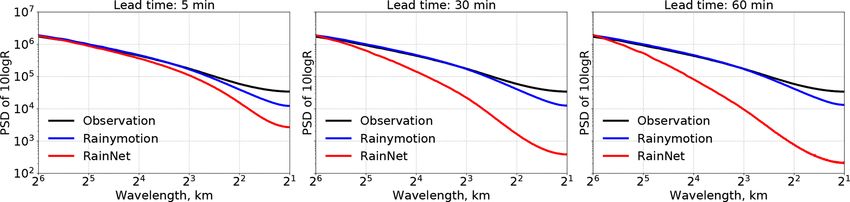
G. Ayzel et al.: RainNet: a convolutional neural network for precipitation nowcasting                                              2635

Figure 2. Illustration of one iteration step of the RainNet parameters optimization procedure.

   We optimized RainNet’s parameters using 10 epochs (one                3     Data and experimental setup
epoch ends when the neural network has seen every input
data sample once; then the next epoch begins) with a mini                3.1    Radar data
batch of size 2 (one mini batch holds a few input data sam-
ples). The optimization procedure converged on the eighth                We use the RY product of the German Weather Service
epoch, showing the saturation of RainNet’s performance on                (DWD) as input data for training and validating the Rain-
the validation data. The learning rate of the Adam optimizer             Net model. The RY product represents a quality-controlled
had a value of 1 × 10⁻⁴ , while other parameters had default             rainfall-depth composite of 17 operational DWD Doppler
values from the original paper of Kingma and Ba (2015).                  radars. It has a spatial extent of 900 km × 900 km, covers the
   The entire setup was empirically identified as the most               whole area of Germany, and has been available since 2006.
successful in terms of RainNet’s performance on validation               The spatial and temporal resolution of the RY product is
data, while other configurations with different loss functions           1 km × 1 km and 5 min, respectively.
(e.g., mean absolute error, mean squared error) and optimiza-               In this study, we use RY data that cover the period from
tion algorithms (e.g., stochastic gradient descent) also con-            2006 to 2017. We split the available RY data as follows:
verged. The average training time on a single GPU (NVIDIA                while we use data from 2006 to 2013 to optimize RainNet’s
GeForce GTX 1080Ti, NVIDIA GTX TITAN X, or NVIDIA                        model parameters and data from 2014 to 2015 to validate
Tesla P100) varies from 72 to 76 h.                                      RainNet’s performance, data from 2016 to 2017 are used for
   We support this paper by a corresponding repository on                model verification (Sect. 3.3). For both optimization and val-
GitHub (https://github.com/hydrogo/rainnet; last access: 10              idation periods, we keep only data from May to September
June 2020; Ayzel, 2020a), which holds the RainNet model                  and ignore time steps for which the precipitation field (with
architecture written in the Python 3 programming language                rainfall intensity more than 0.125 mm h−1 ) covers less than
(https://python.org, last access: 28 January 2020) using the             10 % of the RY domain. For each subset of the data – for
Keras deep learning library (Chollet et al., 2015) alongside             optimization, validation, and verification – every time step
its parameters (Ayzel, 2020b), which had been optimized on               (or frame) is used once as t0 (forecast time) so that the re-
the radar data set described in the following section.                   sulting sequences that are used as input to a single forecast
                                                                         (t0 − 15 min, . . ., t0 ) overlap in time. The number of result-
                                                                         ing sequences amounts to 41 988 for the optimization, 5722
                                                                         for the validation, and 9626 for the verification (see also
                                                                         Sect. 3.3).

https://doi.org/10.5194/gmd-13-2631-2020                                                     Geosci. Model Dev., 13, 2631–2644, 2020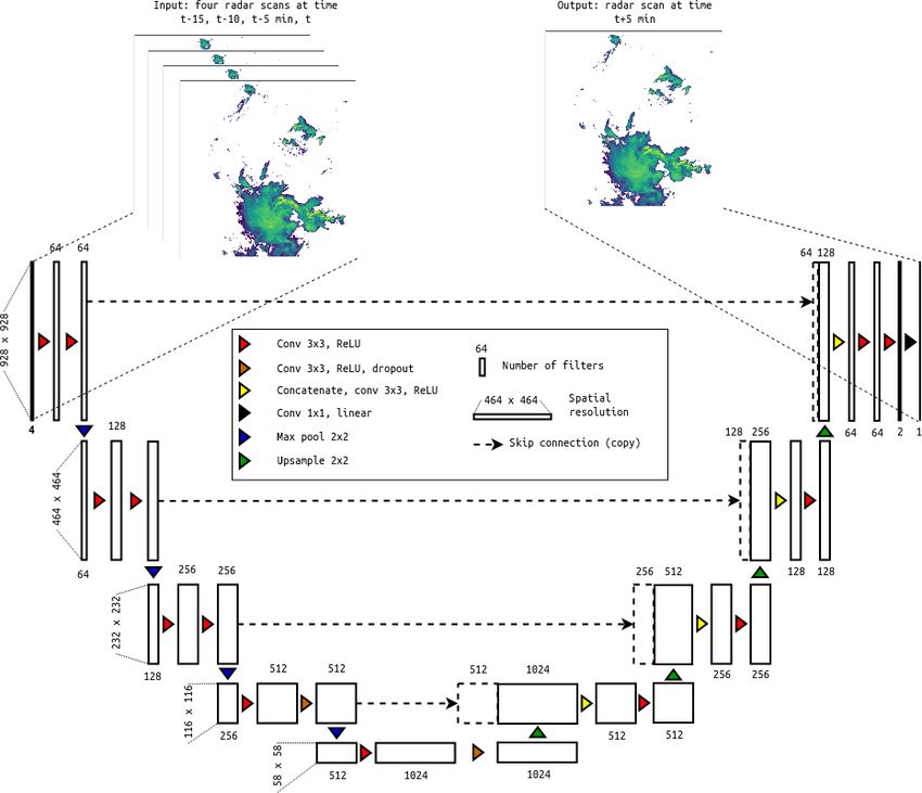
2636 G. Ayzel et al.: RainNet: a convolutional neural network for precipitation nowcasting
3.2 Reference models threshold value. Quantities Pn and Po represent the nowcast
and observed fractions, respectively, of rainfall intensities ex-
We use nowcasting models from the rainymotion Python li- ceeding a specific threshold for a defined neighborhood size.
brary (Ayzel et al., 2019) as benchmarks with which we eval- MAE is positive and unbounded with a perfect score of 0;
uate RainNet. As the first baseline model, we use Eulerian both CSI and FSS can vary from 0 to 1 with a perfect score
persistence (hereafter referred to as Persistence), which as- of 1. We have applied threshold rain rates of 0.125, 1, 5, 10,
sumes that for any lead time n (min) precipitation at t + n and 15 mm h−1 for calculating the CSI and the FSS. For cal-
is the same as at forecast time t. Despite its simplicity, it culating the FSS, we use neighborhood (window) sizes of 1,
is quite a powerful model for very short lead times, which 5, 10, and 20 km.
also establishes a solid verification efficiency baseline which The verification metrics we use in this study quantify the
can be achieved with a trivial model without any explicit as- models’ performance from different perspectives. The MAE
sumptions. As the second baseline model, we use the Dense captures errors in rainfall rate prediction (the fewer the bet-
model from the rainymotion library (hereafter referred to ter), and CSI (the higher the better) captures model accuracy
as Rainymotion), which is based on optical flow techniques – the fraction of the forecast event that was correctly pre-
for precipitation field tracking and the constant-vector ad- dicted – but does not distinguish between the sources of er-
vection scheme for precipitation field extrapolation. Ayzel rors. The FSS determines how the nowcast skill depends on
et al. (2019) showed that this model has an equivalent or both the threshold of rainfall exceedance and the spatial scale
even superior performance in comparison to the operational (Mittermaier and Roberts, 2010).
RADVOR (radar real-time forecasting) model from DWD In addition to standard verification metrics described
for a wide range of rainfall events. above, we calculate the power spectral density (PSD) of now-
casts and corresponding observations using Welch’s method
3.3 Verification experiments and performance (Welch, 1967) to investigate the effects of smoothing demon-
evaluation strated by different models.
For benchmarking RainNet’s predictive skill in comparison
to the baseline models, Rainymotion and Persistence, we se-
lected 11 events during the summer months of the verifica- 4 Results and discussion
tion period (2016–2017). These events were selected for cov-
For each event, RainNet was used to compute nowcasts at
ering a range of event characteristics with different rainfall
lead times from 5 to 60 min (in 5 min steps). To predict the
intensity, spatial coverage, and duration. A detailed account
precipitation at time t + 5 min (t being the forecast time), we
of the events’ properties is given by Ayzel et al. (2019).
used the four latest radar images (at time t − 15, t − 10, and
We use three metrics for model verification: mean abso-
t − 5 min and t) as input. Since RainNet was only trained to
lute error (MAE), critical success index (CSI), and fractions
predict precipitation at 5 min lead times, predictions beyond
skill score (FSS). Each metric represents a different category
t + 5 were made recursively: in order to predict precipita-
of scores. MAE (Eq. 4) corresponds to the continuous cate-
tion at t + 10, we considered the prediction at t + 5 as the
gory and maps the differences between nowcast and observed
latest observation. That recursive procedure was repeated up
rainfall intensities. CSI (Eq. 5) is a categorical score based
to a maximum lead time of 60 min. Rainymotion uses the
on a standard contingency table for calculating matches be-
two latest radar composite grids (t − 5, t) in order to retrieve
tween Boolean variables which indicate the exceedance of
a velocity field and then to advect the latest radar-based pre-
specific rainfall intensity thresholds. FSS (Eq. 6) represents
cipitation observation at forecast time t to t + 5, t + 10, . . . ,
neighborhood verification scores and is based on comparing
and t + 60.
nowcast and observed fractional coverages of rainfall inten-
Figure 3 shows the routine verification metrics MAE and
sities exceeding specific thresholds in spatial neighborhoods
CSI for RainNet, Rainymotion, and Persistence as a function
(windows) of certain sizes.
Pn of lead time. The preliminary analysis had shown the same
|nowi − obsi | general pattern of model efficiency for each of the 11 events
MAE = i=1 , (4)
n (Sect. S1 in the Supplement), which is why we only show the
hits average metrics over all events. The results basically fall into
CSI = , (5) two groups.
hits + false alarms + misses
Pn
(Pn − Po )2 The first group includes the MAE and the CSI metrics
FSS = 1 − Pn i=1 2 Pn 2
, (6) up to a threshold of 5 mm h−1 . For these, RainNet clearly
i=1 Pn + i=1 Po outperforms the benchmarks at any lead time (differences
where quantities nowi and obsi are nowcast and observed between models were tested to be significant with the two-
rainfall rate in the ith pixel of the corresponding radar image, tailed t test at a significance level of 5 %; results not shown).
and n is the number of pixels. Hits, false alarms, and misses Persistence is the least skillful, as could be expected for
are defined by the contingency table and the corresponding a trivial baseline. The relative differences between RainNet
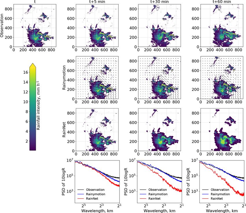
Geosci. Model Dev., 13, 2631–2644, 2020 https://doi.org/10.5194/gmd-13-2631-2020G. Ayzel et al.: RainNet: a convolutional neural network for precipitation nowcasting 2637 and Rainymotion are more pronounced for the MAE than for represents the prominence of precipitation features at differ- the CSI. For the MAE, the advance of RainNet over Rainy- ent spatial scales, expressed as the spectral power at different motion increases with lead time. For the CSI, the superiority wavelengths after a two-dimensional fast Fourier transform. of RainNet over Rainymotion appears to be highest for inter- The power spectrum itself is not of specific interest here; it mediate lead times between 20 and 40 min. The performance is the loss of power at different length scales, relative to the of all models, in terms of CSI, decreases with increasing in- observation, that is relevant in this context. The loss of power tensity thresholds. of Rainymotion nowcasts appears to be constrained to spatial That trend – a decreasing CSI with increasing intensity scales below 4 km and does not seem to depend on lead time – continues with the second group of metrics: the CSI for (see also Ayzel et al., 2019). For RainNet, however, a sub- thresholds of 10 and 15 mm h−1 . For both metrics and any stantial loss of power at length scales below 16 km becomes of the competing methods at any lead time, the CSI does not apparent at a lead time of 5 min. For longer lead times of 30 exceed a value of 0.31 (obtained by RainNet at 5 min lead and 60 min, that loss of power grows and propagates to scales time and a threshold of 10 mm h−1 ). That is below a value of up to 32 km. That loss of power over a range of scales cor- of 1/e ≈ 0.37 which had been suggested by Germann and responds to our visual impression of spatial smoothing. Zawadzki (2002) as a “limit of predictability” (under the as- In order to investigate whether that loss of spectral power sumption that the optimal value of the metric is 1 and that at smaller scales is a general property of RainNet predictions, it follows an exponential-like decay over lead time). Irre- we computed the PSD for each forecast time in each verifica- spective of such an – admittedly arbitrary – predictability tion event in order to obtain an average PSD for observations threshold, the loss of skill from an intensity threshold of 5 and nowcasts at lead times of 5, 30, and 60 min. The corre- to 10 mm h−1 is remarkable for all competing models. Visu- sponding results are shown in Fig. 5. They confirm that the ally more apparent, however, is another property of the sec- behavior observed in the bottom row of Fig. 4 is, in fact, rep- ond group of metrics, which is that Rainymotion outperforms resentative of the entirety of verification events. Precipitation RainNet (except for a threshold of 10 mm h−1 at lead times of fields predicted by RainNet are much smoother than both the 5 and 60 min). That becomes most pronounced for the CSI at observed fields and the Rainymotion nowcasts. At a lead time 15 mm h−1 , while RainNet has a similar CSI value as Rainy- of 5 min, RainNet starts to lose power at a scale of 16 km. motion at a lead time of 5 min, it entirely fails at predicting That loss accumulates over lead time and becomes effective the exceedance of 15 mm h−1 for longer lead times. up to a scale of 32 km at a lead time of 60 min. These results In summary, Fig. 3 suggests that RainNet outperforms confirm qualitative findings of Shi et al. (2015, 2018), who Rainymotion (as a representative of standard tracking and described their nowcasts as “smooth” or “fuzzy”. extrapolation techniques based on optical flow) for low and RainNet obviously learned, as the optimal way to mini- intermediate rain rates (up to 5 mm h−1 ). Neither RainNet mize the loss function, to introduce a certain level of smooth- nor Rainymotion appears to have much skill at predicting the ing for the prediction at time t + 5 min. It might even have exceedance of 10 mm h−1 , but the loss of skill for high in- learned to systematically “attenuate” high intensity features tensities is particularly remarkable for RainNet, which obvi- as a strategy to minimize the loss function, which would ously has difficulties in predicting pronounced precipitation be consistent with the results of the CSI at a threshold of features with high intensities. 15 mm h−1 , as shown in Fig. 3. For the sake of simplicity, In order to better understand the fundamental properties of though, we will refer to the overall effect as “smoothing” RainNet predictions in contrast to Rainymotion, we continue in the rest of the paper. According to the loss of spectral by inspecting a nowcast at three different lead times (5, 30, power, the smoothing is still small at a length scale of 16 km and 60 min) for a verification event at an arbitrarily selected but becomes increasingly effective at smaller scales from 2 forecast time (29 May 2016, 19:15:00 UTC). The top row to 8 km. It is important to note that the loss of power be- of Fig. 4 shows the observed precipitation, and the second low length scales of 16 km at a lead time of 5 min is an es- and third rows show Rainymotion and RainNet predictions. sential property of RainNet. It reflects the learning outcome Since it is visually challenging to track the motion pattern and illustrates how RainNet factors in predictive uncertainty at the scale of 900 km × 900 km by eye, we illustrate the ve- at 5 min lead times by smoothing over small spatial scales. locity field as obtained from optical flow, which forms the Conversely, the increasing loss of power and its propagation basis for Rainymotion’s prediction. While it is certainly dif- to larger scales up to 32 km are not an inherent property of ficult to infer the predictive performance of the two models RainNet but a consequence of its recursive application in our from this figure, another feature becomes immediately strik- study context: as the predictions at short lead times serve as ing: RainNet introduces a spatial smoothing which appears model inputs for predictions at longer lead times, the results to substantially increase with lead time. In order to quan- become increasingly smooth. So while the smoothing intro- tify that visual impression, we calculated, for the same ex- duced at 5 min lead times can be interpreted as a direct re- ample, the power spectral density (PSD) of the nowcasts and sult of the learning procedure, the cumulative smoothing at the corresponding observations (bottom row in Fig. 4), us- longer lead times has to rather be considered an artifact simi- ing Welch’s method (Welch, 1967). In simple terms, the PSD https://doi.org/10.5194/gmd-13-2631-2020 Geosci. Model Dev., 13, 2631–2644, 2020
2638                                    G. Ayzel et al.: RainNet: a convolutional neural network for precipitation nowcasting

Figure 3. Mean absolute error (MAE) and critical success index (CSI) for five different intensity thresholds (0.125, 1, 5, 10, and 15 mm h−1 ).
The metrics are shown as a function of lead time. All values represent the average of the corresponding metric over all 11 verification events.

lar to the effect of “numerical diffusion” in numerically solv-              Based on the above results and discussion of RainNet’s
ing the advection equation.                                               versus Rainymotion’s predictive properties, the FSS figures
   Given this understanding of RainNet’s properties, we used              are plausible and provide a more formalized approach to
the fractions skill score (FSS) to provide further insight into           express different behaviors of RainNet and Rainymotion in
the dependency of predictive skill on the spatial scale. To that          terms of predictive skill. In general, the skill of both mod-
end, the FSS was obtained by comparing the predicted and                  els decreases with decreasing window sizes, increasing lead
observed fractional coverage of pixels (inside a spatial win-             times, and increasing intensity thresholds. RainNet tends to
dow/neighborhood) that exceed a certain intensity threshold               outperform Rainymotion at lower rainfall intensities (up to
(see Eq. 6 in Sect. 3.3). Figure 6 shows the FSS for Rainymo-             5 mm h−1 ) at the native grid resolution (i.e., a window size
tion and RainNet as an average over all verification events,              of 1 km). With increasing window sizes and intensity thresh-
for spatial window sizes of 1, 5, 10, and 20 km, and for in-              olds, Rainymotion becomes the superior model. At an inten-
tensity thresholds of 0.125, 1, 5, 10, and 15 mm h−1 . In addi-           sity threshold of 5 mm h−1 , Rainymotion outperforms Rain-
tion to the color code, the value of the FSS is given for each            Net at window sizes equal to or greater than 5 km. At inten-
combination of window size (scale) and intensity. In the case             sity thresholds of 10 and 15 mm h−1 , Rainymotion is superior
that one model is superior to the other, the correspondingly              at any lead time and window size (except a window size of
higher FSS value is highlighted in bold black digits.                     1 km for a threshold of 10 mm h−1 ).

Geosci. Model Dev., 13, 2631–2644, 2020                                                     https://doi.org/10.5194/gmd-13-2631-2020
G. Ayzel et al.: RainNet: a convolutional neural network for precipitation nowcasting                                                   2639

Figure 4. Precipitation observations as well as Rainymotion and RainNet nowcasts at t = 29 May 2016, 19:15 UTC. Top row: observed
precipitation intensity at time t, t +5, t +30, and t +60 min. Second row: corresponding Rainymotion predictions, together with the underlying
velocity field obtained from optical flow. Bottom row: power spectral density plots for observations and nowcasts at lead times of 5, 30, and
60 min.

Figure 5. PSD averaged over all verification events and nowcasts for lead times of 5, 30, and 60 min.

   The dependency of the FSS (or, rather, the difference of              crease the size of the spatial neighborhood around a pixel,
FSS values between Rainymotion and RainNet) on spatial                   this neighborhood could, at some size, include high-intensity
scale, intensity threshold, and lead time is a direct result             precipitation features that Rainymotion has preserved but
of inherent model properties. Rainymotion advects precip-                slightly misplaced. RainNet’s loss function, however, only
itation features but preserves their intensity. When we in-              accounts for the native grid at 1 km resolution, so it has no

https://doi.org/10.5194/gmd-13-2631-2020                                                     Geosci. Model Dev., 13, 2631–2644, 2020
2640                                    G. Ayzel et al.: RainNet: a convolutional neural network for precipitation nowcasting

Figure 6. Fractions skill score (FSS) for Rainymotion (a, b, c) and RainNet (d, e, f) for 5, 30, and 60 min lead times, for spatial window sizes
of 1, 5, 10, and 20 km, and for intensity thresholds of 0.125, 1, 5, 10, and 15 mm h−1 . In addition to the color code of the FSS, we added the
numerical FSS values. The FSS values of the models which are significantly superior for a specific combination of window size, intensity
threshold, and lead time are typed in bold black digits, and the inferior models are in regular digits.

notion of what could be a slight or “acceptable” displace-                and 5 min in time. Independent verification experiments were
ment error. Instead, RainNet has learned spatial smoothing                carried out on 11 summer precipitation events from 2016 to
as an efficient way to factor in spatial uncertainty and min-             2017. In order to achieve a lead time of 60 min, a recursive
imize the loss function, resulting in a loss of high-intensity            approach was implemented by using RainNet predictions at
features. As discussed above, that effect becomes increas-                5 min lead times as model inputs for longer lead times. In
ingly prominent for longer lead times because the effect of               the verification experiments, Eulerian persistence served as
smoothing propagates.                                                     a trivial benchmark. As an additional benchmark, we used
                                                                          a model from the rainymotion library which had previously
                                                                          been shown to outperform the operational nowcasting model
5   Summary and conclusions                                               of the German Weather Service for the same set of verifica-
                                                                          tion events.
In this study, we have presented RainNet, a deep convolu-
                                                                             RainNet significantly outperformed both benchmark mod-
tional neural network architecture for radar-based precipita-
                                                                          els at all lead times up to 60 min for the routine verification
tion nowcasting. Its design was inspired by the U-Net and
                                                                          metrics mean absolute error (MAE) and the critical success
SegNet families of deep learning models for binary seg-
                                                                          index (CSI) at intensity thresholds of 0.125, 1, and 5 mm h−1 .
mentation, and it follows an encoder–decoder architecture
                                                                          Depending on the verification metric, these results would
in which the encoder progressively downscales the spatial
                                                                          correspond to an extension of the effective lead time in the
resolution using pooling, followed by convolutional layers,
                                                                          order of 10–20 min by RainNet as compared to Rainymo-
and the decoder progressively upscales the learned patterns
                                                                          tion. However, Rainymotion turned out to be clearly superior
to a higher spatial resolution using upsampling, followed by
                                                                          in predicting the exceedance of higher-intensity thresholds
convolutional layers.
                                                                          (here 10 and 15 mm h−1 ) as shown by the corresponding CSI
   RainNet was trained to predict precipitation at a lead time
                                                                          analysis.
of 5 min, using several years of quality-controlled weather
                                                                             RainNet’s limited ability to predict high rainfall intensities
radar composites based on the DWD weather radar net-
                                                                          could be attributed to a remarkable level of spatial smooth-
work. Those data cover Germany with a spatial domain of
                                                                          ing in its predictions. That smoothing becomes increasingly
900 km × 900 km and have a resolution of 1 km in space

Geosci. Model Dev., 13, 2631–2644, 2020                                                      https://doi.org/10.5194/gmd-13-2631-2020
G. Ayzel et al.: RainNet: a convolutional neural network for precipitation nowcasting 2641
apparent at longer lead times. Yet it is already prominent at Net could be trained using precipitation at time t − 15,
a lead time of 5 min. That was confirmed by an analysis of t − 10, . . ., t min as input but using the recursive pre-
power spectral density which showed, at time t +5 min, a loss diction at time t + 5 as an additional input layer. While
of spectral power at length scales of 16 km and below. Obvi- the direct prediction of precipitation at longer lead times
ously, RainNet has learned an optimal level of smoothing to should reduce excessive smoothing as a result of numer-
produce a nowcast at 5 min lead times. In that sense, the loss ical diffusion, we would still expect the level of smooth-
of spectral power at small scales is informative as it reflects ing to increase with lead time as a result of the predictive
the limits of predictability as a function of spatial scale. Be- uncertainty at small scales.
yond the lead time of 5 min, however, the increasing level of
smoothing is a mere artifact – an analogue to numerical diffu- – As an alternative to predicting continuous values of pre-
sion – that is not a property of RainNet itself but of its recur- cipitation intensity, RainNet could be trained to predict
sive application: as we repeatedly use smoothed nowcasts as the exceedance of specific intensity thresholds instead.
model inputs, we cumulate the effect of smoothing over time. That would correspond to a binary segmentation task. It
That certainly is an undesirable property, and it becomes par- is possible that the objective of learning the segmenta-
ticularly unfavorable for the prediction of high-intensity pre- tion for low intensities might be in conflict with learn-
cipitation features. As was shown on the basis of the frac- ing it for high intensities. That is why the training could
tions skill score (FSS), Rainymotion outperforms RainNet be carried out both separately and jointly for disparate
already at an intensity of 5 mm h−1 once we start to eval- thresholds in order to investigate whether there are in-
uate the performance in a spatial neighborhood around the herent trade-offs. From an early warning perspective, it
native grid pixel of 1 km × 1 km size. This is because Rainy- makes sense to train RainNet for binary segmentation
motion preserves distinct precipitation features but tends to based on user-defined thresholds that are governed by
misplace them. RainNet, however, tends to lose such features the context of risk management. The additional advan-
over longer lead times due to cumulative smoothing effects – tage of training RainNet to predict threshold exceedance
more so if it is applied recursively. is that we could use its output directly as a measure of
From an early warning perspective, that property of Rain- uncertainty (of that exceedance).
Net clearly limits its usefulness. There are, however, options
to address that issue in future research. We consider any of those options worth pursuing in order
to increase the usefulness of RainNet in an early warning
– The loss function used in the training could be adjusted
context – i.e., to better represent precipitation intensities that
in order to penalize the loss of power at small spatial
exceed hazardous thresholds. We would expect the overall
scales. The loss function explicitly represents our re-
architecture of RainNet to be a helpful starting point.
quirements to the model. Verifying the model by other
Yet the key issue of precipitation prediction – the antici-
performance metrics will typically reveal whether these
pation of convective initialization, as well as the growth and
metrics are rather in agreement or in conflict with these
dissipation of precipitation in the imminent future – still ap-
requirements. In our case, the logcosh loss function ap-
pears to be unresolved. It is an inherent limitation of nowcast-
pears to favor a low MAE but at the cost of losing
ing models purely based on optical flow: they can extrapolate
distinct precipitation features. In general, future users
motion fairly well, but they cannot predict intensity dynam-
need to be aware that, apart from the network design,
ics. Deep learning architectures, however, might be able to
the optimization itself constitutes the main difference to
learn recurrent patterns of growth and dissipation, although
“heuristic” tracking-and-extrapolation techniques (such
it will be challenging to verify if they actually did. In the con-
as Rainymotion) which do not use any systematic pa-
text of this study, though, we have to assume that RainNet has
rameter optimization. The training procedure will stub-
rather learned the representation of motion patterns instead
bornly attempt to minimize the loss function, irrespec-
of rainfall intensity dynamics: for a lead time of 5 min, the
tive of what researchers consider to be “physically plau-
effects of motion can generally be expected to dominate over
sible”. For many researchers in the field of nowcast-
the effects of intensity dynamics, which will propagate to the
ing, that notion might be in stark contrast to experiences
learning results. The fact that we actually could recursively
with “conventional” nowcasting techniques which tend
use RainNet’s predictions at 5 min lead times in order to pre-
to effortlessly produce at least plausible patterns.
dict precipitation at 1 h lead times also implies that RainNet,
– RainNet should be directly trained to predict precipita- in essence, learned to represent motion patterns and optimal
tion at lead times beyond 5 min. However, preliminary smoothing. In that case, the trained model might even be ap-
training experiments with that learning task had diffi- plicable on data in another region, which could be tested in
culties to converge. We thus recommend to still use re- future verification experiments.
cursive predictions as model inputs for longer lead times Another limitation in successfully learning patterns of in-
during training in order to improve convergence. For ex- tensity growth and dissipation might be the input data itself.
ample, to predict precipitation at time t + 10 min, Rain- While we do not exclude the possibility that such patterns
https://doi.org/10.5194/gmd-13-2631-2020 Geosci. Model Dev., 13, 2631–2644, 20202642 G. Ayzel et al.: RainNet: a convolutional neural network for precipitation nowcasting
could be learned from just two-dimensional radar compos- Competing interests. The authors declare that they have no conflict
ites, other input variables might add essential information on of interest.
imminent atmospheric dynamics – the predisposition of the
atmosphere to produce or to dissolve precipitation. Such ad-
ditional data might include three-dimensional radar volume Acknowledgements. Georgy Ayzel would like to thank the Open
data, dual-polarization radar moments, or the output fields of Data Science community (https://ods.ai, last access: 10 June 2020)
numerical weather prediction (NWP) models. Formally, the for many valuable discussions and educational help in the grow-
ing field of deep learning. We ran our experiments using the GPU
inclusion of NWP fields in a learning framework could be
computation resources of the Machine Learning Group of the Uni-
considered as a different way of assimilation, combining –
versity of Potsdam (Potsdam, Germany) and the Shared Facility
in a data-driven way – the information content of physical Center “Data Center of FEB RAS” (Khabarovsk, Russia). We ac-
models and observations. knowledge the support of Deutsche Forschungsgemeinschaft (Ger-
Our study provides, after Shi et al. (2015, 2017, 2018), man Research Foundation) and the open-access publication fund of
another proof of concept that convolutional neural networks the University of Potsdam.
provide a firm basis to compete with conventional nowcast-
ing models based on optical flow (most recently, Google Re-
search has also reported similar attempts based on a U-Net Financial support. This research has been supported by Geo.X, the
architecture; see Agrawal et al., 2019). Yet this study should Research Network for Geosciences in Berlin and Potsdam (grant no.
rather be considered as a starting point to further improve the SO_087_GeoX).
predictive skill of convolutional neural networks and to better
understand the properties of their predictions – in a statistical
sense but also in how processes of motion and intensity dy- Review statement. This paper was edited by Simone Marras and re-
namics are reflected. To that end, computational complexity viewed by Scott Collis and Gabriele Franch.
and the cost of the training process still have to be considered
as inhibitive, despite the tremendous progress achieved in the
past years. RainNet’s training would require almost a year
on a standard desktop CPU in contrast to 3 d on a modern
References
desktop GPU (although the latter is a challenge to implement
for non-experts). Yet it is possible to run deep learning mod-
Agrawal, S., Barrington, L., Bromberg, C., Burge, J., Gazen, C., and
els with already optimized (pretrained) weights on a desktop Hickey, J.: Machine Learning for Precipitation Nowcasting from
computer. Thus, it is important to make available not only Radar Images, available at: https://arxiv.org/abs/1912.12132 (last
the code of the network architecture but also the correspond- access: 28 January 2020), 2019.
ing weights, applicable using open-source software tools and Austin, G. L. and Bellon, A.: The use of digital
libraries. We provide all this – code, pretrained weights, as weather radar records for short-term precipitation
well as training and verification data – as an input for future forecasting, Q. J. Roy. Meteor. Soc., 100, 658–664,
studies on open repositories (Ayzel, 2020a, b, c). https://doi.org/10.1002/qj.49710042612, 1974.
Ayzel, G.: hydrogo/rainnet: RainNet v1.0-gmdd, Zenodo,
https://doi.org/10.5281/zenodo.3631038, 2020a.
Code and data availability. The RainNet model is free and open Ayzel, G.: RainNet: pretrained model and weights, Zenodo,
source. It is distributed under the MIT software license which https://doi.org/10.5281/zenodo.3630429, 2020b.
allows unrestricted use. The source code is provided through Ayzel, G.: RYDL: the sample data of the RY
a GitHub repository https://github.com/hydrogo/rainnet (last ac- product for deep learning applications, Zenodo,
cess: 30 January 2020; Ayzel, 2020d); a snapshot of RainNet v1.0 https://doi.org/10.5281/zenodo.3629951, 2020c.
is also available at https://doi.org/10.5281/zenodo.3631038 (Ayzel, Ayzel, G.: RainNet: a convolutional neural network for radar-
2020a); the pretrained RainNet model and its weights are available based precipitation nowcasting, available at: https://github.com/
at https://doi.org/10.5281/zenodo.3630429 (Ayzel, 2020b). DWD hydrogo/rainnet, last access: 10 June 2020.
provided the sample data of the RY product; it is available at Ayzel, G., Heistermann, M., and Winterrath, T.: Optical flow mod-
https://doi.org/10.5281/zenodo.3629951 (Ayzel, 2020c). els as an open benchmark for radar-based precipitation now-
casting (rainymotion v0.1), Geosci. Model Dev., 12, 1387–1402,
https://doi.org/10.5194/gmd-12-1387-2019, 2019.
Badrinarayanan, V., Kendall, A., and Cipolla, R.: SegNet: A
Supplement. The supplement related to this article is available on-
Deep Convolutional Encoder-Decoder Architecture for Im-
line at: https://doi.org/10.5194/gmd-13-2631-2020-supplement.
age Segmentation, IEEE T. Pattern Anal., 39, 2481–2495,
https://doi.org/10.1109/TPAMI.2016.2644615, 2017.
Bai, S., Kolter, J. Z., and Koltun, V.: An Empirical Evaluation of
Author contributions. GA developed the RainNet model, carried Generic Convolutional and Recurrent Networks for Sequence
out the benchmark experiments, and wrote the paper. TS and MH Modeling, available at: https://arxiv.org/abs/1803.01271 (last ac-
supervised the study and co-authored the paper. cess: 28 January 2020), 2018.
Geosci. Model Dev., 13, 2631–2644, 2020 https://doi.org/10.5194/gmd-13-2631-2020G. Ayzel et al.: RainNet: a convolutional neural network for precipitation nowcasting 2643 Bauer, P., Thorpe, A., and Brunet, G.: The quiet revolu- 4824-imagenet-classification-with-deep-convolutional-neural-networks. tion of numerical weather prediction, Nature, 525, 47–55, pdf (last access: 10 June 2020), 2012. https://doi.org/10.1038/nature14956, 2015. LeCun, Y., Bengio, Y., and Hinton, G.: Deep learning, Nature, 521, Boureau, Y.-L., Ponce, J., and LeCun, Y.: A Theoretical Analysis 436–444, https://doi.org/10.1038/nature14539, 2015. of Feature Pooling in Visual Recognition, in: Proceedings of the Lin, C., Vasić, S., Kilambi, A., Turner, B., and Zawadzki, I.: Pre- 27th International Conference on International Conference on cipitation forecast skill of numerical weather prediction mod- Machine Learning, ICML’10, Omnipress, Madison, WI, USA, els and radar nowcasts, Geophys. Res. Lett., 32, L14801, 21–24 June 2010, Haifa, Israel, 111–118, 2010. https://doi.org/10.1029/2005GL023451, 2005. Chen, P., Chen, G., and Zhang, S.: Log Hyperbolic Cosine Long, J., Shelhamer, E., and Darrell, T.: Fully Convolutional Net- Loss Improves Variational Auto-Encoder, available at: https:// works for Semantic Segmentation, in: The IEEE Conference on openreview.net/forum?id=rkglvsC9Ym (last access: 28 January Computer Vision and Pattern Recognition (CVPR), 8–12 June 2020), 2018. 2015, Boston, Massachusetts, USA, 2015. Chollet, F. et al.: Keras, https://keras.io (last access: 10 June 2020), Mittermaier, M. and Roberts, N.: Intercomparison of Spatial Fore- 2015. cast Verification Methods: Identifying Skillful Spatial Scales Us- Dahl, G. E., Sainath, T. N., and Hinton, G. E.: Improving deep neu- ing the Fractions Skill Score, Weather Forecast., 25, 343–354, ral networks for LVCSR using rectified linear units and dropout, https://doi.org/10.1175/2009WAF2222260.1, 2010. in: 2013 IEEE International Conference on Acoustics, Speech Nair, V. and Hinton, G. E.: Interpersonal Informatics: Making So- and Signal Processing, 26–31 May 2013, Vancouver, Canada, cial Influence Visible, in: Proceedings of the 27th International 8609–8613, https://doi.org/10.1109/ICASSP.2013.6639346, Conference on International Conference on Machine Learning, 2013. ICML’10, Omnipress, Madison, WI, USA, 21–24 June 2010, Dueben, P. D. and Bauer, P.: Challenges and design choices Haifa, Israel, 807–814, 2010. for global weather and climate models based on ma- Reichstein, M., Camps-Valls, G., Stevens, B., Jung, M., Denzler, J., chine learning, Geosci. Model Dev., 11, 3999–4009, Carvalhais, N., and Prabhat: Deep learning and process under- https://doi.org/10.5194/gmd-11-3999-2018, 2018. standing for data-driven Earth system science, Nature, 566, 195– Gehring, J., Auli, M., Grangier, D., Yarats, D., and Dauphin, Y. N.: 204, https://doi.org/10.1038/s41586-019-0912-1, 2019. Convolutional Sequence to Sequence Learning, in: Proceedings Reyniers, M.: Quantitative precipitation forecasts based on of the 34th International Conference on Machine Learning – Vol- radar observations: Principles, algorithms and operational sys- ume 70, ICML’17, 6–11 August 2017,Sydney, Australia, 1243– tems, Institut Royal Météorologique de Belgique, available 1252, JMLR.org, 2017. at: https://www.meteo.be/meteo/download/fr/3040165/pdf/rmi_ Gentine, P., Pritchard, M., Rasp, S., Reinaudi, G., and Ya- scpub-1261.pdf (last access: 10 June 2020), 2008. calis, G.: Could Machine Learning Break the Convection Pa- Ronneberger, O., Fischer, P., and Brox, T.: U-Net: Convolutional rameterization Deadlock?, Geophys. Res. Lett., 45, 5742–5751, Networks for Biomedical Image Segmentation, in: Medical Im- https://doi.org/10.1029/2018GL078202, 2018. age Computing and Computer-Assisted Intervention – MICCAI Germann, U. and Zawadzki, I.: Scale-Dependence of the 2015, edited by: Navab, N., Hornegger, J., Wells, W. M., and Predictability of Precipitation from Continental Radar Frangi, A. F., Springer International Publishing, Cham, pp. 234– Images. Part I: Description of the Methodology, Mon. 241, https://doi.org/10.1007/978-3-319-24574-4_28, 2015. Weather Rev., 130, 2859–2873, https://doi.org/10.1175/1520- Shi, E., Li, Q., Gu, D., and Zhao, Z.: A Method of Weather Radar 0493(2002)1302.0.CO;2, 2002. Echo Extrapolation Based on Convolutional Neural Networks, Gu, J., Wang, Z., Kuen, J., Ma, L., Shahroudy, A., Shuai, B., Liu, T., in: MultiMedia Modeling, edited by: Schoeffmann, K., Chalid- Wang, X., Wang, G., Cai, J., and Chen, T.: Recent advances abhongse, T. H., Ngo, C. W., Aramvith, S., O’Connor, N. E., in convolutional neural networks, Pattern Recogn., 77, 354–377, Ho, Y.-S., Gabbouj, M., and Elgammal, A., Springer Interna- https://doi.org/10.1016/j.patcog.2017.10.013, 2018. tional Publishing, Cham, pp. 16–28, https://doi.org/10.1007/978- Iglovikov, V. and Shvets, A.: TernausNet: U-Net with VGG11 En- 3-319-73603-7_2, 2018. coder Pre-Trained on ImageNet for Image Segmentation, avail- Shi, X., Chen, Z., Wang, H., Yeung, D.-Y., Wong, W.-k., and able at: https://arxiv.org/abs/1801.05746 (last access: 28 January Woo, W.-c.: Convolutional LSTM Network: A Machine Learn- 2020), 2018. ing Approach for Precipitation Nowcasting, in: Advances in Kingma, D. P. and Ba, J.: Adam: A Method for Stochastic Opti- Neural Information Processing Systems 28, edited by: Cortes, C., mization, in: 3rd International Conference on Learning Repre- Lawrence, N. D., Lee, D. D., Sugiyama, M., and Garnett, R., Cur- sentations, ICLR 2015, San Diego, CA, USA, 7–9 May 2015, ran Associates, Inc., Red Hook, NY, USA, 802–810, available at: Conference Track Proceedings, edited by: Bengio, Y. and Le- http://papers.nips.cc/paper/5955-convolutional-lstm-network- Cun, Y., available at: http://arxiv.org/abs/1412.6980 (last access: a-machine-learning-approach-for-precipitation-nowcasting.pdf 10 June 2020), 2015. (last access: 10 June 2020), 2015. Krizhevsky, A., Sutskever, I., and Hinton, G. E.: ImageNet Shi, X., Gao, Z., Lausen, L., Wang, H., Yeung, D.-Y., Wong, W.-k., Classification with Deep Convolutional Neural Networks, and Woo, W.-c.: Deep Learning for Precipitation Nowcasting: A in: Advances in Neural Information Processing Systems 25, Benchmark and A New Model, in: Advances in Neural Informa- NIPS 2012, Lake Tahoe, Nevada, USA, 3–9 December 2012, tion Processing Systems 30, edited by: Guyon, I., Luxburg, U. V., Curran Associates, Inc. Red Hook, NY, USA, edited by: Bengio, S., Wallach, H., Fergus, R., Vishwanathan, S., and Gar- Pereira, F., Burges, C. J. C., Bottou, L., and Weinberger, nett, R., Curran Associates, Inc., Red Hook, NY, USA, K. Q., 1097–1105, available at: http://papers.nips.cc/paper/ 5617–5627, available at: http://papers.nips.cc/paper/7145-deep- https://doi.org/10.5194/gmd-13-2631-2020 Geosci. Model Dev., 13, 2631–2644, 2020
You can also read