Unravel Tax Planning Differences between Multinational and Domestic Firms

Unravel Tax Planning Differences between Multinational and Domestic Firms

 Working Paper
 – January 2019 –

 Christoph Watrin
 University of Münster
 christoph.watrin@wiwi.uni-muenster.de

 Falko Weiß*
 University of Münster
 falko.weiss@wiwi.uni-muenster.de

*
 Corresponding author: Institute of Accounting and Taxation, Universitätsstraße 14-16,
D-48143 Münster, Germany. E-mail: falko.weiss@wiwi.uni-muenster.de
Phone: +49(0)251-83-22031. Fax: +49(0)251-83-21824.

Abstract: Prior literature primarily identifies tax planning via an analysis of the firms’ effective tax
rate (ETR) or variations of it. However, several disadvantages go along with ETRs like the exclusion
of loss-firms (equal to 30% of the sample) or a mismeasurement of corporate tax planning which
stems from truncating ETRs as pointed out by Henry and Sansing (2014). In this paper, we develop
a new measure suitable to overcome these shortcomings. Another advantage is the separation of a
firm’s tax planning activity into a time-invariant idiosyncratic component and a characteristic-var-
ying component. The first should be associated with the firm’s tax strategy as a firm characteristic
while the second should show any single-year effects as a reaction to a change of firm characteristics
or external events/shocks. We present a comparison between the new measure and other tax plan-
ning measures like single-year/long-rung GAAP- and Cash ETR or Book-Tax Differences. By man-
ually seeding artificial tax planning activity into the data, we provide evidence that the new measure
might be a better indicator to identify tax planning than variations of the ETR. Further, we apply the
measure in a subsequent analysis to evaluate differences between tax planning behavior of multina-
tional and domestic firms. We provide evidence that no structural difference exist between both
groups and present a possible explanation for differences resulting from an analysis with ETRs. We
identify effects of double taxation and foreign tax credits to be of major importance if comparing
multinational and domestic firms.
JEL Classification: H21, H25, H26, M40, M41
Keywords: Tax Planning, Measure Tax Planning, Simulated Data, Seeding Artificial Tax Planning,
Time-invariant versus Characteristic-varying Tax Planning, Multinationals vs. Domestics

Acknowledgments: We thank the participants of the 41st Annual Congress of the European Ac-
counting Association in Milan, the 2018 Annual Conference of the Canadian Academic Accounting
Association in Calgary, the Sixth International Conference of the Journal of International Account-
ing Research in Venice, the Tax Research Network 2018 Annual Conference in Birmingham and
the National Tax Association’s 111th Annual Conference in New Orleans for their helpful com-
ments. We especially appreciate the valuable suggestions by Alex Edwards and Cristi Gleason. This
research did not receive any specific grant from funding agencies in the public, commercial, or not-
for-profit sector.

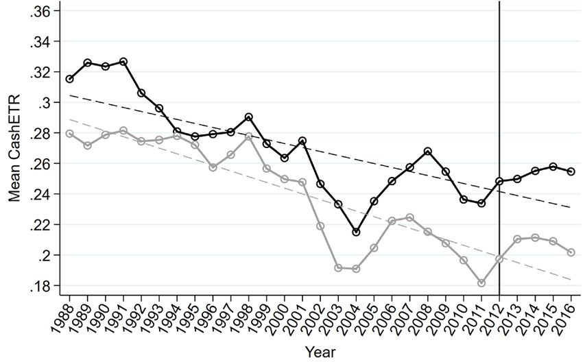
1 Introduction

Starting with the elementary question whether taxes matter or not, a wide stream of literature

has risen to find answers to this question. The problem with evaluating the corporate tax plan-

ning behavior is the nature of this characteristic. No company reports the amount of taxes they

avoided due to tax planning, nor do they report the effort they put into tax savings strategies.

The firms’ tax planning activities are unobservable for researchers or policy makers, while

highly relevant on the other hand. However, the basic question, how to infer the underlying

strategies when you cannot observe tax planning, does not seem to be answered. Hanlon and

Heitzman (2010) call for further research in the area of how to measure tax planning.

Prior literature primarily employs the effective tax rate (ETR) as an indicator to measure tax

planning activities. Dyreng, Hanlon, Maydew and Thornock (2017) provide an analysis of the

Cash ETR’s changes over the past 25 years and interpret a negative slope as a hint towards

growing tax planning activity across the sample. The technical construction of an ETR means

several limitations resulting in a bias and misleading interpretations. Henry and Sansing (2014)

show that dropping all firm-year observations with negative pre-tax income results in such a

bias when it comes to evaluating tax planning activities. Prior studies regularly drop observa-

tions with negative pre-tax income. Therefore, they derive their universal inferences from a

biased subsample. The handling of loss firm-years is crucial when deriving inferences valid for

the whole population. The portion of loss firms is highly correlated with year-mean effective

tax rates. Therefore, this paper introduces a new measure to identify the effect of tax planning

and those companies associated with an engagement in such strategies while accounting for

loss firms-years.

The paper contributes to the literature in three major ways. First, it introduces a new tax plan-

ning measure. The development of a new measure enables new opportunities and methods of

 1

measuring relations and associations between certain firm characteristics and tax planning be-

havior. Researchers benefit from a tax planning measure, which incorporates a time-invariant

tax planning component which does not change over time while simultaneously providing a

characteristic-varying component which identifies single-year effects. The rationale behind this

differentiation is the nature of tax planning. Some studies define tax planning as a firm charac-

teristic which is associated with other firm specific attributes and is therefore less likely to

change every year (low volatility is desired). This idea is captured by the time-invariant tax

planning component and is of low 1 variation for each firm over the sample period. However,

this component does not capture tax planning entirely. Due to changes in the firm specific at-

tributes or other environmental incidents, a firm’s tax planning characteristic may change. To

capture this characteristic, the new tax planning measure includes a characteristic-varying tax

planning component. This component expresses any tax planning activities – either a reduction

or an increase – deviating from the average firm level. The combination enables the analysis of

research questions where both aspects are of relevance for the researcher.

For most prior research, the source of tax related information is the GAAP financial statement.

This information might differ from those reported in the tax return files due to different disclo-

sure regulations. Additionally, the management might have some incentives to actively manage

not only earnings but also reported tax information. Therefore, we do not want to rely on total

tax expense or current tax expense since these information might be subject to such manage-

ment activity. Dhaliwal, Gleason and Mills (2004) confirm this assumption showing that the

GAAP tax accounts might be subject to earnings management. Rather, we employ cash taxes

paid as the amount really paid to the tax authorities. The problem with cash taxes paid is the

nature of this position because the amount paid in the current period is not only induced by the

1
 In theory there would be no variation at all. Since we scale the fixed-effects by taxes paid (which varies from
 year to year) the resulting time-invariant tax planning estimation also shows small variation.
 2

current period’s GAAP revenue as reported in the financial statement. The elementary idea

behind the new tax planning measure is that a tax payment is determined by the corresponding

GAAP-reported pre-tax income of that period and the GAAP-reported pre-tax income of pre-

vious periods due to retrospective tax payments. Dyreng, Hanlon and Maydew (2008) already

present a method to account for intertemporal associations by calculating a long-run effective

rate. The paramount idea was the elimination of outliers and the identification of a firm’s tax

planning behavior following the understanding of a more constant characteristic. However, we

do not know to which extent the tax payment is related to the different periods’ pretax incomes.

One would suggest that the essential part of cash taxes paid in the current period depends on

pre-tax income as reported in the tax return files. Back taxes and deferred revenue seem to be

subordinate to current year’s tax expense. However, the exact composition of cash taxes paid

does not seem to be clear from a theoretical point of view. To shed light into the composition,

cash taxes paid is the dependent variable in our pooled cross-sectional OLS estimation. 2 The

lagged and current pre-tax income of this firm serve as independent variables to estimate the

respective coefficients. In a second step, the estimated coefficients are used to predict cash taxes

paid in a firm-fixed effects model. The firm-fixed effects serve as the proxy for time-invariant

tax planning while the residuals serve as a proxy for characteristic-varying tax planning both

resulting in the Relative Tax Planning Measure (RTPM). Overall, this measure enables a sim-

ultaneous evaluation of both tax planning components.

Since the interpretation of negative effective tax rates is problematic and effective tax rates

greater than one are difficult to handle, ETRs are regularly truncated (e.g., Bauer (2015); Cheng,

Huang, Li, and Stanfield (2012); Davis, Guenther, Krull, and Williams (2016); Hoi, Wu, and

Zhang (2013); McGuire, Omer, and Wang (2012); Robinson, Sikes, and Weaver (2010)) or

2
 Although current year’s tax expense is owed on income measured by tax law cash taxes paid also contain back
 tax payments violating a strict matching principle.
 3

censored at zero and one (e.g., Armstrong, Blouin, and Larcker (2012); Badertscher, Katz, and

Rego (2013); Brown and Drake (2014); Dyreng, Hanlon, and Maydew (2010); Gaertner (2014);

Gallemore and Labro (2015); Higgins, Omer, and Phillips (2015); Hope, Ma, and Thomas

(2013); McGuire, Wang, and Wilson (2014)). The adjustment of the data results in a truncation

bias, as pointed out by Henry and Sansing (2014). According to their study, observations with

negative pre-tax income or tax refunds are positively associated with tax planning. If just drop-

ping all these information or replacing the information by a value of zero limits the explanatory

power and regularly underestimates the association with tax planning. Such a bias resulting in

an underestimation does not occur using RTPM. 3

Following the presentation of the new measure, we present a data manipulation method already

introduced by DeSimone, Nickerson, Seidman and Stomberg (2016) to validate the appropri-

ateness of the new measure. The enhancement of this method represents the second contribution

to the literature. By artificially seeding additional tax avoidance into the sample, we evaluate

in a logistic regression if our new tax planning measure identifies tax planning behavior. A

comparison with some ETR variations (single-year/long-run Cash/GAAP ETR) and book-tax

differences demonstrate the robustness and appropriateness of our new measure. We suggest

that our new measure is able to identify such additionally seeded tax planning while other

measures partly fail to show any significant associations while others provide weak evidence.

In the last step, we apply the new RTPM measure to evaluate potential differences in tax plan-

ning behavior for multinational and domestic firms. This analysis represents the third contribu-

tion to the tax planning literature. We provide evidence that no structural difference exists be-

tween both groups of firms as indicated by employing the Cash ETR. Differences resulting from

such an analysis may be explained by a missing separation into foreign and domestic pre-tax

3
 Since consecutive firm-year observations are necessary, the new way of identifying tax planning does also limit
 the data. However, the advantage is that the loss of data is not associated with tax planning and therefore does
 not result in a systematic bias and an underestimation of tax planning.
 4

income or cash taxes paid. Our analysis hints towards different effects of foreign pre-tax income

compared to domestic pre-tax income on cash taxes paid. Double taxation may explain these

differences. Furthermore, tax credits granted due to foreign cash taxes paid do not reduce do-

mestic cash taxes paid correspondingly resulting in a further need to differentiate between do-

mestic and foreign nature. It seems that significant differences between domestics’ and multi-

nationals’ tax planning behavior occur in times of crises like the Tech-Bubble, the 2008-finan-

cial crises or the Flash-Crash in 2011.

The paper proceeds as follows: In chapter 2, we present already established measures to identify

tax planning. Chapter 3 introduces the new measure, its theoretical as well as the empirical

construction. Chapter 4 compares the appropriateness of RTPM in identifying tax planning with

other measures. Chapter 5 employs the new measure to analyze the development of tax plan-

ning with a comparison of multinational firms with domestic firms while chapter 6 concludes.

2 Methods of Measuring Tax Planning

Prior literature reviews (e.g., Shackelford and Shevlin (2001); Hanlon and Heitzman (2010))

provide a good overview about the widely accepted proxies presenting their strengths and lim-

itations for tax planning. This chapter will not discuss those strengths and weaknesses in detail

but summarize the most important measures to capture tax planning. The focus lies on the

measure itself and not on studies evaluating any relations with other firm characteristics or

further tax planning determinants.

The information source for any analysis regarding tax planning can either be the tax return file

or the financial statement. Hanlon and Heitzman (2010) discuss the sources’ quality in detail

and state that it is nearly impossible to match information from both types due to different

consolidation rules. Lots of studies state that information from the tax return files would be of

relevance and the desired source. However, these information are hard to get since they are
 5

confidential and only a very limited number of changing researchers is granted access to these

information. The limited access is the next problem arising when employing confidential data

since the resulting study is not replicable. As a consequence, the majority of studies utilize data

from the financial statements. This approach is not uncontroversial since financial disclosure

does not require any information regarding cash taxes paid for current year’s return. Hanlon

and Heitzman (2010) explain this lack of information by the focus of the FASB. The board aims

to demand for all information necessary to evaluate the economic performance for stakeholders

and to enable them to generate accurate future forecasts. It seems that cash taxes paid for a

fiscal year is what investors are interested in. Hanlon (2003) and McGill and Outslay (2004)

discuss such problems arising from utilizing financial data for taxable income forecasts. Nev-

ertheless, the advantage of applying financial statement data is the broad availability and there-

fore, this source of information is widely accepted and used in prior literature.

Early studies employ simple measures like taxes paid or ratios like effective tax rates. The nu-

merator defines the type of ETR. If worldwide total tax expense is scaled by worldwide total

pre-tax income, the resulting ratio is the GAAP ETR. A disadvantage of utilizing the GAAP ETR

is that strategies deferring taxes are not captured by the proxy since total tax expense contains

the deferred tax component. Hanlon and Heitzman (2010) list some items which are typically

not tax planning instruments but affect the GAAP ETR (e.g. changes in the valuation allowance

or changes in the tax contingency reserve). Next to the GAAP ETR, the Cash ETR is the second

common ratio widely used to capture tax planning, avoidance, aggressiveness or burden. In-

stead of worldwide total tax expense, worldwide income taxes paid is scaled by worldwide total

pre-tax income. One benefit of the alternative ratio is that deferral strategies affect the Cash

ETR. However, a mismatch of the nominator and denominator is the result of pre-tax earnings

being a single (current) year information while cash taxes paid relate to several (prior and cur-

rent) periods due to subsequent payments of taxes.

 6

De Simone et al. (2016) argue that the method of limiting the ETR is essential for the statistical

power of the model and for the possibility of identifying any effect. Truncating, winsorizing or

deleting extreme values has a substantial effect on the model and the findings. Therefore, one

should carefully think about the right method for ensuring that the data fits to the interpretability

of the results. Furthermore, Henry and Sansing (2014) express skepticism to trust the Cash ETR

because of the transformation necessary to enable the calculation of the ratio. Deleting or win-

sorizing extreme values decreases not only the variance, but also destructs essential information

about outliers. They caution about a potential bias between extreme ETR values and the under-

lying tax planning behavior. A further limitation accrues from the type of tax planning the

measure is capable to detect. The Cash ETR as well as the GAAP ETR measure share the dis-

advantage of only capturing non-conforming tax planning as the denominator is the pre-tax

income, which might already be managed via conforming tax planning. Although not highly

problematic for public companies it is not possible to detect conforming tax planning with both

measures.

Dyreng et al. (2008) recommend averaging the information over longer periods to avoid singly-

year outliers and extreme values. In their study, the authors sum up cash taxes paid as well as

pre-tax income over a period of 3/10 years. This new interpretation of an effective tax rate as a

measure of firm-average tax planning overcomes some interpretation problems since the ETR

is smoothed over several years and outliers are also eliminated while volatility is reduced. This

enhancement of the single-year ETR has another advantage for the Cash ETR. Hanlon and

Heitzman (2010) review a reduction in the timing mismatch between cash taxes paid and pre-

tax income. Due to the advantages just presented, a broad majority of researchers adopted the

long-run measure for their analyses in the following years (e.g., Rego and Wilson (2012); Ba-

dertscher et al. (2013); Brown and Drake (2014)). Nevertheless, the advantage of smoothed

 7

ETRs is a disadvantage at the same time. The loss of information content makes it nearly im-

possible to evaluate single-year effects or direct effects of external events.

Another modification is the calculation of a tax rate differential. Subtracting the effective tax

rate from the statutory tax rate yields the differential. Those companies showing a positive dif-

ferential (lower ETR than the statutory tax rate) may be engaged in tax planning activities.

However, there are some limitations applying such a comparison. If the officially defined tax

base is lower than the pretax income reported in the annual report due to tax exemptions and

deductions, the ETR will be lower than the statutory tax rate by default. 4 The taxation system

of the United States is characterized by one of the highest tax rates in the world while allowing

for several tax base deductions like permanently reinvested earnings. Due to the number of

exemptions, one would not expect the average company to report an ETR of 35% 5. To address

this problem of relativity and increase comparability among firms Armstrong, Blouin, Jago-

linzer, and Larcker (2015) present a peer-specific adjustment of a firm’s mean or median ETR.

They construct a tax avoidance proxy defined as the difference between a firm’s three-year

GAAP ETR and the average GAAP ETR of the firm’s peer group by size and industry.

As stated in the introduction of this chapter, financial statement information and tax return in-

formation cannot be matched due to different disclosure requirements. Therefore, the difference

between taxable income in the tax return file and pre-tax income in the financial statement can

yield information regarding the tax planning activity. Book-tax differences (BTD) are calcu-

lated as pre-tax book income minus the difference of current tax expense scaled by the statutory

tax rate and the change in net operating loss. This idea has already been employed by Mills

(1998) who identified an association between BTD and the probability to being audited by the

IRS. Wilson (2009) documents higher levels of BTD for those firms engaged in tax shelters.

4
 De Simone et al. (2016) list some of these exemptions: tax credits, the domestic production activities deduction
 or an investment in tax-exempt securities reduce the tax base in a way desired and allowed by the government.
5
 The statutory tax rate refers to the sample period until 2016 without considering recent legal changes.
 8

The studies suggest that BTD – at least to some extend – capture tax planning activity. However,

as Hanlon and Heitzman (2010) state, the capital market pressure limits the appropriateness of

BTD. Therefore, only firms with similar importance on financial accounting earnings can be

compared using BTD. This makes the measure inappropriate for samples widely differing in

capital market pressure. 6 Next to the just presented total book tax difference, temporary BTD

are calculated by scaling deferred tax with the statutory tax rate. Similar to the detection ability

of ETRs, total and temporary BTD are only suitable to capture non-conforming tax planning

activities.

As an extension to the idea of book-tax differences, Desai and Dharmapala (2006, 2009) con-

struct abnormal BTD via including a correction for accounting earnings management. They

regress total BTD on total accruals and define the residuals as abnormal BTD. Also Frank,

Lynch and Rego (2009) define the residuals of their first stage regression (multiply the differ-

ence between the effective tax rate and the statutory tax rate with the pre-tax income and regress

this expression over a set of control variables) to be the tax planning variable of interest. They

name the residuals of this regression DTAX and define it to show any intentional tax planning

activity. Hanlon and Heitzman (2010) pronounce that one needs to be careful when defining

such a setting. Since it is not obvious which components to include in the first stage model and

which components to load in the residuals, the interpretation might be difficult. In a recent

study, Chen, Hribar and Melessa (2018) call for caution when generating residuals in a first

stage regression to employ them in a second stage regression. Due to the possible bias with the

dependent variable in the first regression the second stage results might show incorrect infer-

ences.

Unrecognized tax benefits (UTB) define another variable which has been used by prior litera-

ture to detect tax planning activity. The accounting reserve for uncertainty in future income

6
 This is not as important if comparing public companies only.
 9

taxes is highly sensitive to accounting earnings management since it affects bottom-line earn-

ings. Therefore, this position might be relevant for earnings management rather than a proxy

for tax planning activity. If employing UTB in a research setting and deriving inferences,

Hanlon and Heitzman (2010) suggest to account for this dual nature and discuss the implica-

tions in detail instead of ignoring the earnings management component and declare the variable

to be a tax planning indicator. Hutchens and Rego (2015) present a set of determinants to detect

tax risk one of which being UTB. Employing several measures is another way to account for

the unclear role of UTB for the firm’s top management.

Another group of tax planning indicators are tax shelter activities which represent the “aggres-

sive” or non-conforming end of the tax planning continuum. These methods detect firms which

are engaged in specific tax shelter activities. Wilson (2009) presents a score derived from cer-

tain firm characteristics which detects tax shelter activity and predicts the probability of an

engagement in tax shelter activities. Hanlon and Heitzman (2010) present two major disad-

vantages of such measures. The potential selection bias is a severe statistical problem. Infor-

mation regarding specific tax shelters are only available, if a firm is either caught or discloses

the shelter activity. The second problem with tax shelter scores is the nature of endogeneity.

Only if firms are not able to achieve the desired level of tax efficiency 7 via less “aggressive”

strategies a firm is willing to engage in single tax shelter transactions. Therefore, the tax shelter

activity does not directly refer to a certain level of company tax planning activity but present a

punctual tax “aggressive” transaction next to a certain level of the company’s tax planning be-

havior.

7
 Tax efficiency refers to increasing after tax returns. Therefor taxes are evaluated as an expense position, which
 should be minimized to increase shareholder value.
 10

Several different measures overcoming different shortcomings exist to capture tax planning.

Although some are supposed to measure the same, the results strongly differ. Hanlon and Heit-

zman (2010) point out that one should be careful in choosing the right measure that fits the

research question. The just presented measures show low correlations although they are sup-

posed to measure the same. Thus, Hanlon and Heitzman (2010) call for further research on tax

planning measures.

3 Development of the Relative Tax Planning Measure

3.1 Fundamental Idea behind “Relative Tax Planning”

We follow the understanding of tax planning as a continuum drawn by Hanlon and Heitzman

(2010). Similar to other studies, the aim of this study is to identify tax planning regardless of

being at the conforming or “aggressive” end of the continuum. Therefore, we use the term tax

planning to describe a reduction in tax payments regardless of the strategy undertaken.

To enable a replication of our results and a broad use of the measure, our source of data are

financial statements rather than tax return files. Using financial statement data calls for caution

regarding the informative content. Some key data seem to be more relevant but less reliable

while others seem to be more reliable but less relevant. When it comes to tax positions, the

GAAP ETR seems to more adequately address the principle of causation and attribute the taxes

to the respective periods. However, the GAAP ETR is not as reliable as the Cash ETR since it

is subject to the management’s judgement. Although managed GAAP pre-tax income is the

denominator for both measures, GAAP ETR also contains an information subject to manage-

ment’s estimation in the nominator. On the other hand, the Cash ETR is more reliable than the

GAAP ETR due to the nature of actually being paid. However, this ratio might be less relevant

because of the timing mismatch between the nominator and denominator. The amount of cash

taxes paid in a period does not only depend on the pre-tax income from that period. Due to
 11

subsequent tax payments prior years’ pre-tax income also affect current year’s cash taxes paid.

Prior studies like Dhaliwal et al. (2004) confirm this assumption and provide evidence that tax

expense information are subject to earnings management. Therefore, we do not want to rely on

total tax expense, current tax expense or deferred tax expense. Instead, the amount of taxes

actually paid to the tax authority is the information of interest (higher reliability). We account

for the timing mismatch via defining cash taxes paid as a function of prior years’ and next year’s

pre-tax income. This approach allows us to employ cash taxes paid while considering the inter-

temporal nature of the cash position (increase relevance). At the same time, we do not need to

rely on (possibly) managed amounts in the financial reports.

The argument for employing cash taxes paid is the exclusion of current or total tax expense due

to the possibility of being managed. Managed information make it impossible to interpret re-

sulting effects. Hanlon and Heitzman (2010) argue that a differentiation between “aggressive”

(upward) earnings management and “aggressive” (downward) tax planning is not possible since

both result in lower ETRs. It is not clear, whether management actively optimized the nomina-

tor or denominator.

Another advantage along with our intertemporal interpretation of cash taxes paid is that we do

not need to drop all firm-year observations with negative pre-tax income as done in prior studies

(e.g. Badertscher et al. (2013), Cheng et al. (2012), Dyreng et al. (2010), Hoi et al. (2013),

Hoopes, Mescall and Pittman (2012), Hope et al. (2013), McGuire et al. (2012) and McGuire

et al. (2014)) or tax refunds (Cheng et al. (2012), Hoi et al. (2013), Hope et al. (2013) and

McGuire et al. (2012)). An indicator variable for loss firms enables the special treatment of loss

firms when it comes to tax questions. Therefore, results drawn from employing the new meas-

ure do not only hold for profitable firms but for loss firms as well. Further, no bias due to the

exclusion of loss firms causes distorted results and estimates. Our proxy for tax planning should

be unbiased with loss firms and the pre-tax income.

 12

The tax planning measure should provide an intuition for a firm’s tax planning behavior in

relation to other companies as well as in relation to its own (past) tax planning behavior. There-

fore, the model provides a time-invariant component expressing the firm’s average tax planning

level in relation to others (all other companies or the industry peer-group). It would be quite

naïve not to allow for a changing tax planning behavior. Hanlon and Heitzman (2010) argue

that the level of tax planning depends on certain internal and external characteristics. These

might change over time. Therefore, the second tax planning component addresses this require-

ment and expresses any deviations from the firm specific time-invariant tax planning level.

While the relative understanding of tax planning is a major strength of the new measure, it is

necessary to mention that it also has a limitation. If all firms reduce their tax liabilities analog-

ically, the new measure might not identify the tax planning activity.

3.2 Technical Construction of the Relative Tax Planning Measure

The tax burden a company has to face is defined by the taxable income and the statutory tax

rate (τ). For reasons of data availability and replicability, we approximate the taxable income

by the GAAP pre-tax income. Since the sample consists of US corporations only, τ equals a

constant term 0.35 and, technically, reduces pretax income to 35% and defines this amount as

tax expense. 8 However, several exceptions and firm specific peculiarities make it impossible to

estimate taxes paid by multiplying the pre-tax income with the statutory tax rate. An unobserv-

able factor which accounts for any deviations from the statutory tax rate needs to be considered,

the adjustment term a. This term comprises tax effective reductions like permanently reinvested

earnings. Prior literature therefore defines the Cash ETR as the product of τ and a which is

8
 For simplicity we refrain from distinguishing between various state tax rates. Different statutory tax-rates across
 countries can be modeled by including in the regression function. Such an inclusion also enables tax-rate changes
 over time.
 13

calculated dividing TXPD by PI. Equation (1) shows the idea of thinking about tax planning as

an additional term to calculate the tax burden.

 = ∗ ∗ (1)

As shown in the literature review section, prior studies regularly apply a variation of the ex-

pression in Equation (1) defined as worldwide cash taxes paid divided by pre-tax income (Cash

ETR). This approach displays a, which is responsible for any deviations from the statutory tax

rate, together with the statutory tax rate in one expression ( ℎ = ∗ = / ).

Dyreng and Lindsey (2009) rearrange this expression for their analysis to come back to the idea

of calculating the tax burden. We follow their approach and do not display the adjustment term

with the statutory tax rate but express a together with pretax income as shown in Equation (1).

While prior literature applies worldwide cash taxes paid, we estimate domestic cash taxes paid

to enable a comparison of multinational firms with domestic firms. The amount of foreign cash

taxes paid depends on the countries a company pays taxes in and the respective tax rates. In

addition, the relative composition influences the foreign tax burden. Excluding foreign cash

taxes paid from the left side of the equation makes companies comparable – the multinationals

with one another and with domestic firms. Since the United States are characterized by a world-

wide tax system the amount of domestic cash taxes paid may be explained by domestic pre-tax

income and foreign pre-tax income. However, foreign taxes need to be considered as well since

foreign tax credits may reduce the domestic tax burden.

Since tax regulations differentiate between gains, which are subject to taxation, and losses,

which are not, Equation (2) presents this estimation considering the special role of losses via

including an indicator variable LOSS equal to one for firms with a negative pre-tax income and

zero for firms with positive pre-tax income. Since most double taxation arrangements do not

 14

allow a consideration of foreign losses, we apply an interaction with domestic pre-tax income

instead of worldwide pre-tax income. 9

 , = 0 + 1 , + 1 , + 1 , ∗ , + 1 , + 1 , 
 (2)
 + ����������������⃗
 + , 

However, cash taxes paid is not only characterized by accounting transactions in year t but also

includes prior year’s pretax income due to subsequent tax payments. The amount of income

taxes paid by company i in time t constitutes the dependent variable (TXPDDOM). The dependent

variable is explained by the domestic and foreign pretax income (PIDOM and PIFO) in time t-3,

t-2, t-1, t and t+1. For the special treatment of loss firms we incorporate the loss indicator

variable in time t and the interaction with domestic pre-tax income in time t. Equation (3) illus-

trates the regression model to determine the coefficients for estimating domestic cash taxes

paid.

 +1 +1
 
 , = 0 + ⃗ � 
 , + ⃗ � 
 , 
 + 1 , , + 1 , 
 =−3 =−3

 (3)
 + 1 , + 1 , + 2 , + 3 , + 4 , 

 + 5 , + 6 , + 7 , + + , 

The OLS estimation model yields beta and gamma coefficients 1 to 5. 1 ( 1) shows how the

amount of domestic taxes paid in time t is influenced by domestic (foreign) pre-tax income in
 
time t-3. Variable , indicates the amount of domestic taxes paid by company i in time

t. ,[ −3; −2; −1; ; +1] is the domestic pretax income of company i in t [-3, -2, -1, 0, +1] while

 ,[ −3; −2; −1; ; +1] is the foreign pretax income of company i in t [-3, -2, -1, 0, +1]. , 

is the foreign cash taxes paid by company i in t. The control variables are SIZE which is defined

as the natural logarithm of total assets, LEV is defined as total long-term debt scaled by total

9
 Untabulated regression results suggest that it does not matter whether to interact loss with domestic or worldwide
 pre-tax income. The statistical significance is the same yielding a slightly higher coefficient.
 15

assets, PPE represents property, plant and equipment also scaled by total assets, INTAN is de-

fined as total intangible assets scaled by total assets and CASH represents the company’s cash

scaled by total assets. GROWTH is defined as the growth rate of pre-tax income and NOL rep-

resents the net income if it is smaller than zero.

The panel regression estimates Equation (3) as a firm-fixed effects model. By running the re-

gression as a firm-fixed effects model, the regression estimates the coefficients, which equal a

multiplier similar to the effective tax rate but only including characteristic-varying effects.

Firm-specific time-invariant effects will be attributed to the firm-fixed effects.

Equation (3) provides an estimation of domestic cash taxes paid depending on several years’

domestic and foreign pre-tax income. After estimating the coefficients presented in Equation

(3), these coefficients are used to predict the amount of estimated domestic cash taxes paid in

 � ) given the pretax income in periods t-3 to t+1 for each firm-year observation.
time t ( , 

This estimation of domestic cash taxes paid refers to the relative amount of taxes a firm should

pay in year t given the information on domestic and foreign pre-tax income for the current and

three prior years, foreign cash taxes paid, the loss situation and a set of control variables for the

current year.

In analogy to Choudhary, Koester, and Shevlin (2016) who develop a proxy for tax accrual

quality we are primary interested in the residuals of Equation (3) instead of the coefficients.

The residuals of this estimation represent the deviation of the estimated amount of taxes paid

from the real amount of taxes paid. However, applying the firm-fixed effects model, the resid-

uals are adjusted for time-invariant deviations. Therefore, the residuals show characteristic-

varying deviations, only. These characteristic-varying deviations are multiplied with -1 to be

positive if taxes paid is smaller than estimated taxes paid. Such an observation is labeled “tax

planning”. Since a certain deviation can only be evaluated in relation to the estimated amount

of taxes paid, the residuals are standardized by dividing them by the amount of taxes paid. The
 16

scaling with cash taxes paid which has been the dependent variable in the first stage regression

enables an unbiased interpretation of the residuals. 10

 , 
 , = ∗ (−1)
 �������������
 � (4)
 , 

However, the second dimension needs to be considered if evaluating firm-year observations in

a panel structure. Having estimated the characteristic-varying tax planning behavior, the time-

invariant firm-specific tax planning behavior is also of interest. Therefore, the firm-specific

estimated fixed effects serve as an indicator for time-invariant tax planning. In analogy to the

characteristic-varying estimation, the time-invariant deviations are multiplied with -1 to be pos-

itive if taxes paid is smaller than estimated taxes paid. Also, a normalization with taxes paid

yields a relative indicator.

 , = ∗ (−1)
 �������������
 � 
 (5)
 , 

Having estimated the characteristic-varying and time-invariant amount of tax planning for each

company in each year, adding both effects results in the final tax planning measure RTPM for

firm i in time t.

 − , − −( , + )
 , = , + , = + = (6)
 ������������� �������������
 � � �������������
 � 
 , , , 

The result of Equation (6) represents the new relative tax planning measure (RTPM). If the

value is greater than the mean, tax planning is indicated for a company. Values lower than the

mean indicate that the company is paying more taxes than expected based on the regression

from Equation (3).

10
 Chen et al. (2018) suggest to normalize residuals with the dependent variable to avoid a bias in later regressions.
 17

3.3 Sample and Descriptive Statistics

The sample is drawn from Compustat North America providing consolidated firm-year obser-

vations for active US companies. To enable a long-term perspective and replicate the findings

on tax planning for domestic firms versus multinational firms from Dyreng et al. (2017) we

need the analysis to start in 1988 and range until 2016 since data for 2017 provides insufficient

information. For setting up the new measure, 3 lagged and one lead period are necessary result-

ing in a total (applicable) sample period from 1985 to 2016 (1988 to 2015). The unbalanced

sample yields 211,329 firm-year observations in total. As done in prior studies we exclude firms

from the finance and assurance sector (less 53,758 observations). For setting up the new tax

planning measure, we lose years 1985-1987 and 2016 with 21,303 firm-year observations. Also,

five consecutive firm-year observations are necessary (less 32,997 observations) along with

information on the control variables (less 10,074 observations). The final number of firm-year

observations therefore is 93,197. The aim of this paper is to present the relative tax planning

measure. Therefore, a comparison with established tax planning measures should validate the

new measure. Table (1) provides a summary of descriptive statistics for the new relative tax

planning measure, a set of tax planning measures and the variables used for setting up RTPM.

The first row reports the descriptive statistics for RTPM. In total 93,197 firm-year observations

provide information on RTPM. The mean value of RTPM is 0.4587 with a standard variation of

1.8 ranging from -8.5 to 8.4. RTPMfirm and RTPMtime are the two components summing up to

the relative tax planning measure. While RTPMfirm has a similar mean as RTPM, it is not sur-

prising that the firm-fixed component is characterized by a lower standard deviation only rang-

ing from -3.8 to 3.6. In contrast, RTPMtime has a mean of approximately 0 with a high standard

variation ranging from -7.5 to 7.2. Turning to the effective tax rates yields a consistent picture

compared to prior literature. The single-year and long-run ETRs are truncated at 0 and 1 and

 18

therefore limit the number of observations. While the structural loss of data is not as severe for

the GAAP ETR the long-run Cash ETR shows 74,114 observations only. The mean effective

tax rate ranges from 26.47% for the Cash ETR to 33.76% for the GAAP ETR. Book-tax differ-

ences are available for 138,521 observations while providing a mean of 18.989 with a high

standard deviation of 737. Information on cash taxes paid is available for 144,171 firm-year

observations with a mean of 45.037. TXPDDOM is calculated as total cash taxes paid minus

foreign cash taxes paid resulting in the same number of observations as TXPD but a lower mean

of 32.4. TXPDFO is equal to zero if a firm did does not report any foreign cash taxes paid. The

number of observations therefore equals the sample size and the mean value becomes very

small with 5.8. A similar picture occurs for pre-tax income and the separation into a domestic

and a foreign portion. While information on PI is available for 199,270 firm-year observations

the mean for total pre-tax income is 136.85 and for domestic pre-tax income 106.74. foreign

pre-tax income is calculated in analogy to foreign cash taxes paid resulting in 216,541 obser-

vations with a mean of 16.52. Since unprofitable firms are excluded for any analyses employing

various ETR measures the final variable LOSS is an indicator variable equal to 1 in case of

negative pre-tax income and zero otherwise. The mean of 0.319 indicates that nearly one third

of all firm-year observations are loss-firms which are structurally excluded if working with

single-year ETRs.

In Table (2), the Spearman and Pearson correlations are presented. The Spearman correlations

are reported below the diagonal and the Pearson correlations are reported above the diagonal.

RTPM shows a high correlation with RTPMfirm and RTPMtime what is not surprising since it is

the sum of both. If comparing RTPM with the different effective tax rates, one would expect a

higher association with Cash ETR than with GAAP ETR, since taxes paid is a component of

both, RTPM and Cash ETR. The association with book-tax differences is very low but with the

 19

predicted sign. The correlation matrix underlines the statement by Hanlon and Heitzman

(2010): Although the measures of tax planning are supposed to measure the same, they vary in

terms of assumptions and informative content.

3.4 Results of Constructing RTPM

Table (3) presents the regression results applying an ordinary least squares estimation model.

Robust standard errors are applied for the fixed effects (FE) model. Column (1) reports the

coefficients from regressing Equation (3) while Column (2) reports the t-statistics. Column (3)

shows the regression without control variables and Column (4) presents the corresponding t-

statistics.

For the main regression, 93,197 firm-year observations are available resulting in an adjusted R2

of 72.27%. 72% of the variation in TXPDDOM can be explained by the domestic and foreign pre-

tax income from the current, prior three and next year as well as the loss indicator with the

interaction term and the control variables. The regression coefficients and their signs for the

current, lagged and leading pre-tax income are consistent with intuition. Both, domestic and

foreign pre-tax income seem to increase domestic cash taxes paid. Looking at domestic pre-tax

income first, most impact stems from current year’s pre-tax income with yearly decreasing im-

pacts through t-3 and lowest coefficient in t+1. Current year’s domestic cash taxes paid com-

prises 8.1% of current year’s domestic pre-tax income, 6.6% of last year’s domestic income,

approximately 2% of domestic pre-tax income in t-2 and t-3 and 1.5% of next year’s domestic

income. All coefficients are statistically significant on a level of 1%.

Since the United States are characterized by a worldwide taxation system, foreign pre-tax earn-

ings also affect domestic cash taxes paid. In contrast to domestic pre-tax income, domestic cash

 20

taxes paid is associated with current year’s and prior years’ foreign pre-tax income while pre-

tax income in t+1 do not seem to be associated with TXPDDOM. Current year’s domestic cash

taxes paid further comprises 7.6% of current year’s foreign pre-tax income (1% significance

interval), 8.8% of last year’s domestic income (1% significance interval) and approximately

3.5% of domestic pre-tax income in t-2 (1% significance interval) and t-3 (5% significance

interval). Again, all coefficients show positive signs indicating that foreign pre-tax income in-

creases the tax burden at home. When applying foreign pre-tax earnings in the equation, foreign

cash taxes paid need to be considered as well. Foreign tax credits may reduce the tax liability

at home and therefore a negative sign is predicted for an association of foreign cash taxes paid

with domestic cash taxes paid. Indeed, the coefficient is negative with statistical significance

on a level of 1%. The coefficient needs to be interpreted as follows: Current year’s domestic

cash taxes paid are reduced by 75.2% of foreign cash taxes paid. The coefficient seems to make

sense. This may be a hint towards double taxation for multinational companies which are not

able to fully deduct foreign tax expense. This may also be an indicator for higher tax rates for

multinational firms. Domestic firms do not run into double taxation for domestic pre-tax in-

come.

The loss indicator variable does not provide any statistical significance. However, the interac-

tion term with domestic pre-tax income provides a negative coefficient on a significance level

of 1%. A company’s loss in the current period seems to be associated with an increase in cash

taxes paid by 10% of the loss. 11 The negative sign indicates the special role of loss firms if it

comes to taxation. Not allowing for a different treatment via another coefficient would lead to

11
 The negative coefficient is necessary to offset the implied tax refund by β4 (PIDOM in t) and prior years’ induced
 effect on cash taxes paid.
 21

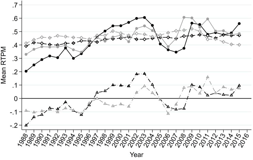
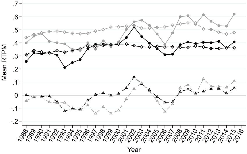
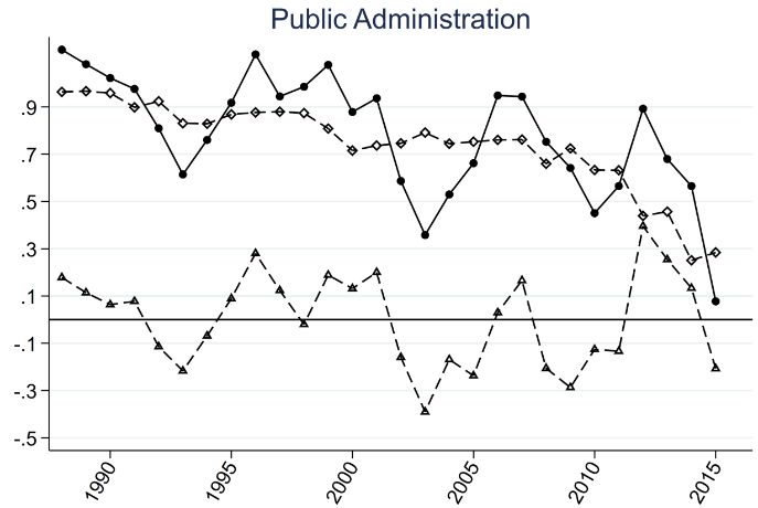
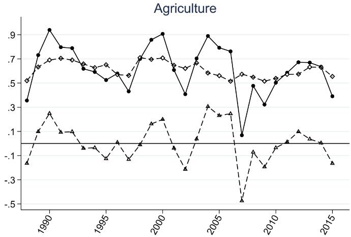
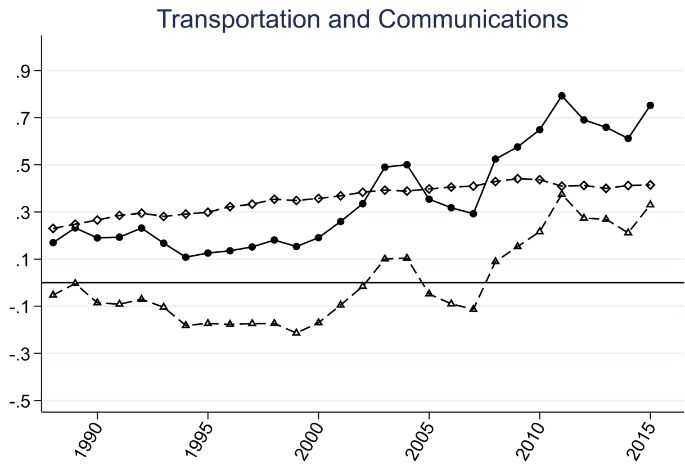
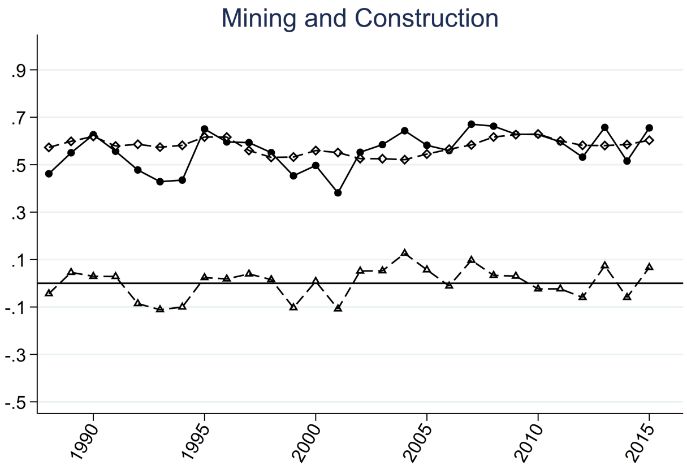
identical coefficients for profitable firm-year observations as for non-profitable ones. There-

fore, the positive coefficient would indicate negative cash taxes paid similar in magnitude to

profitable firms in the presence of a loss year resulting in a corresponding tax refund.

For the control variables, only SIZE, CASH, GROWTH and NOL provide significant coeffi-

cients indicating that domestic cash taxes paid increases with firm size and the growth rate

while decreases with the amount of cash held by the company and net operating losses.

As a robustness test, the variation of Equation (3) provides the same regression without incor-

porating control variables. According to our theory, control variables should not explain our

results and the associations of pre-tax income with domestic cash taxes paid. Although SIZE,

CASH, GROWTH and NOL are statistically significant on a level of at least 5%, the results from

a regression without control variables underline the findings from column (1). A comparison of

the respective coefficients yields the same statistical power with similar statistical and econom-

ical significance. The adjusted R2 slightly decreases by 0.73 percentage points. As indicated by

the comparison, the control variables do not explain much variation in the dependent variable

or drive the significance or magnitude of the coefficients of interest. Due to the explanatory

power provided by SIZE, CASH, GROWTH and NOL we proceed with the model definition as

shown in Equation (3) containing the set of control variables.

Figure (1) presents the development of RTPM over time by plotting yearly mean values. The

illustration provides a first impression for a slightly rising time-varying tax planning component

which constantly jumps around zero. Characteristic-varying tax planning seems to be constant

over time while the combination of both slightly increases over time.

The model specification with firm-fixed effects does not allow for industry specific adjustments

or industry-fixed effects. Structural differences across industries may be possible and should be

 22

controlled for. Therefore, Figure (2) provides a graphical illustration of RTPM, RTPMfirm and

RTPMtime for each industry separately.

While some industries are characterized by high volatility (Agriculture and Public Administra-

tion) others show extremely low variation over time (Trade and Services). In addition, the de-

velopment over time seems to be different across industries. While for example Transportation

and Communication seem to increase the tax planning activity over time, Trade seems to lower

tax planning while Mining and Construction or Services seem to hold a constant level. The

graphical analysis provides some evidence that a difference tax planning behavior may exist

across industries. To address this finding, we modify our estimation of domestic cash taxes paid

in the regression model following Equation (3) by running the model per industry.

Table (4) presents the regression coefficients after running Equation (3) within each industry.

The number of observations within each industry varies between 425 (Agriculture, Forestry and

Fishing) and 41,874 (Manufacturing). The adjusted R2 also varies between 92.1% (Agriculture,

Forestry and Fishing) and 56.8% (Public Administration). Overall, less coefficients seem to be

statistically significant while still providing good adjusted R2. Taken together, the coefficients

on domestic pre-tax income confirm prior findings across all industries. Nevertheless, foreign

pre-tax earnings seem to be especially relevant for Manufacturing. The findings on the loss

interaction term still hold and foreign tax credits seem to be relevant for all industries but Trans-

portation and Communication. The regression results hint towards a different composition of

domestic cash taxes paid. Therefore, running the regression to estimate RTPM should be done

per industry to allow for other coefficients and industry-specific specialties. Running the main

model per industry yields a similar picture as provided in Figure (1).

 23

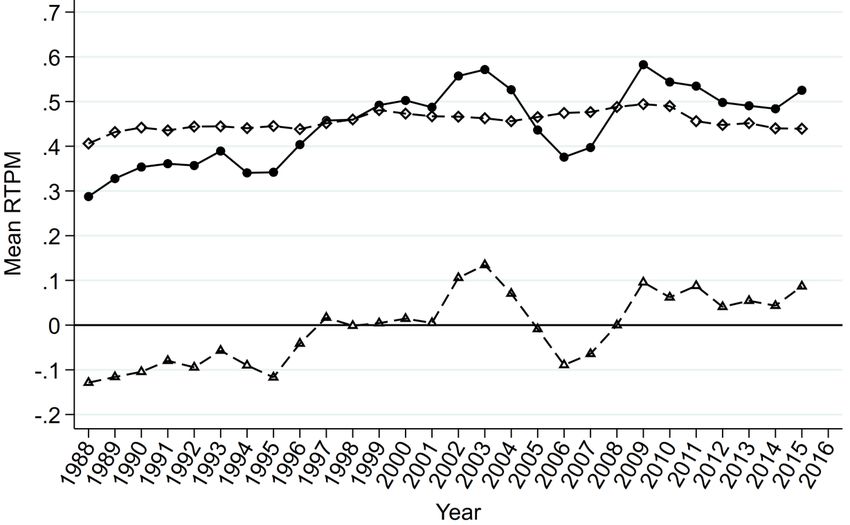
Figure (3) presents yearly mean tax planning after having estimated domestic cash taxes paid

per industry. Although time-varying tax planning shows a similar movement around zero as

shown in Figure (1), the amplitude seems to be bigger. Consequently, the volatility of RTPM is

higher if running the model per industry.

4 Appropriateness of RTPM: Seeding Artificial Tax Planning

4.1 Idea of Artificially Seeding Tax Planning Behavior

A major problem evaluating the quality of a tax planning measure is verification. Since the

“real” tax planning strategy or an intrinsic tax planning behavior of a firm is not known, the

classification of one measure as superior is difficult. However, De Simone et al. (2016) present

the idea of artificially “seeding” additional tax planning into a given sample. Randomly treating

some observations with additional tax planning enables a comparison of how different measures

identify the treated firms. Having seeded additional tax planning for a known treatment group

enables to check for better detection of these treated firms.

De Simone et al. (2016) combine an allocation of additional tax planning following a permanent

avoidance strategy, a temporary avoidance strategy which reverses in the next year and a com-

bination of both. In analogy to their approach, we employ three different seeding methods to

mimic diverse strategies for reducing a firm’s tax position. We seed artificial tax planning fol-

lowing (1) a single-year reduction of taxes, (2) a reversal strategy, which reduces the tax posi-

tion in the year of the treatment but increases the tax position in the next year, and (3) a perma-

nent reduction of taxes, which equals a reduction of the tax position in every year following the

treatment.

Randomly, numbers following a normal distribution with an expectation value of -1 and a stand-

ard deviation of 1 are allocated to each firm-year. Each positive value identifies the treatment

 24

(approximately 15% of the sample). All firm-years allocated to the treatment group receive a

reduction of their tax positon. Not changing the pre-tax income, cash taxes paid, current tax

expense and total tax expense are reduced to mimic an additional tax planning activity. The

amount of the reduction equals 3% of the pre-tax earnings the firm faces in the year of the

treatment. In case of a single-year reduction the tax position is reduced in the year of treatment

only. When applying the reverting reduction, the treated firms receive a reduction (as calculated

above) in the year of the treatment while receiving an increase in the tax position by the same

amount one year after the treatment. The permanent reduction decreases the firms’ tax position

not only in the year of the treatment but also for all following years (by the previously calculated

amount).

A logistic regression should provide possible associations between the treatment (having re-

ceiving artificial tax planning) and the respective measure for identifying tax planning. The

measures should detect tax planning activities. Knowing which observations received such an

additional reduction of the tax position we can evaluate the detection of the various tax planning

measures.

 treatmenti,t = β0 + β1 i,t + β2 SIZEi,t +
 (7)
 β3 ROAi,t + β4 LEVi,t + β5 PPE + β6 INTAN + β7 CASH + β8 GROWTH + εi,t
 i,t i,t i,t i,t

If the respective measure adequately identifies tax planning, statistically significant results

should document such ability. Receiving the treatment is explained by the respective tax plan-

ning measure (TPM) and a set of control variables as shown in the logistic regression in Equa-

tion (9).

4.2 Regression Results on Seeding Artificial Tax Planning

 25

Table (5) presents the logistic regression results for explaining the probability of having re-

ceived the treatment of additional tax planning as the dependent variable. To address concerns

of multicollinearity the logit model regresses the treatment indicator on each tax planning meas-

ure separately.

The first column estimates the logit model with the Cash ETR as the independent variable

along with a set of control variables. Column (2) presents the regression with the long-run Cash

ETR as the independent variable while Column (3)/ (4)/ (5) and (6) explain the indicator varia-

ble for having received the treatment via the GAAP ETR/ long-run GAAP ETR/ BTD and RTPM.

The logistic regression provides statistically significant (1% confidence interval) coefficients

for all six tax planning measures indicating an association of the various measures with addi-

tionally seeded tax planning. The first row provides the marginal effects of the respective tax

planning measure. Again, all coefficients are significant on a level of 1%. The marginal effect

needs to be interpreted as follows: An increase of the Cash ETR by 1% is associated with a

decrease in probability of having received the treatment of 0.03%. The margins are estimated

at means and therefore not as easy to interpret for the whole sample. The important notion here

is that statistical significance is indicated for all tax planning measures.

To get an impression for the suitability of the different tax planning measures we apply the

various measures and mark those firm-years for which the measure detects tax planning. In a

second step, we look at all firm-year observations, which have received the treatment and com-

pare the number of detections by the various measure. Table (6) only reports firm-years, with a

treatment.

 26