Simulating compound weather extremes responsible for critical crop failure with stochastic weather generators - Earth System Dynamics
←
→
Page content transcription
If your browser does not render page correctly, please read the page content below
Earth Syst. Dynam., 12, 103–120, 2021
https://doi.org/10.5194/esd-12-103-2021
© Author(s) 2021. This work is distributed under
the Creative Commons Attribution 4.0 License.

       Simulating compound weather extremes responsible for
        critical crop failure with stochastic weather generators
          Peter Pfleiderer1,2,3 , Aglaé Jézéquel4,5 , Juliette Legrand6 , Natacha Legrix7,8 , Iason Markantonis10 ,
                                           Edoardo Vignotto9 , and Pascal Yiou6
                                            1 Climate     Analytics, Berlin, Germany
                            2 Department     of Geography, Humboldt University, Berlin, Germany
                  3 Earth System Analysis, Potsdam Institute for Climate Impact Research, Potsdam, Germany
                    4 LMD/IPSL, ENS, PSL Université, École Polytechnique, Institut Polytechnique de Paris,

                                         Sorbonne Université, CNRS, 75005 Paris, France
                                  5 École des Ponts Paristech, 77420 Champs-sur-Marne, France
                 6 Laboratoire des Sciences du Climat et de l’Environnement, UMR8212 CEA-CNRS-UVSQ,

                                      IPSL & U Paris-Saclay, 91191 Gif-sur-Yvette, France
             7 Climate and Environmental Physics, Physics Institute, University of Bern, Bern, 3012, Switzerland
                 8 Oeschger Centre for Climate Change Research, University of Bern, Bern, 3012, Switzerland
                        9 Research Center for Statistics, University of Geneva, Geneva, 1211, Switzerland
         10 INRASTES Department, National Centre of Scientific Research “Demokritos”, Aghia Paraskevi, Greece

                        Correspondence: Peter Pfleiderer (peter.pfleiderer@climateanalytics.org)

                                   Received: 28 May 2020 – Discussion started: 10 June 2020
                     Revised: 13 November 2020 – Accepted: 16 December 2020 – Published: 2 February 2021

      Abstract. In 2016, northern France experienced an unprecedented wheat crop loss. The cause of this event is
      not yet fully understood, and none of the most used crop forecast models were able to predict the event (Ben-Ari
      et al., 2018). However, this extreme event was likely due to a sequence of particular meteorological conditions,
      i.e. too few cold days in late autumn–winter and abnormally high precipitation during the spring season. Here
      we focus on a compound meteorological hazard (warm winter and wet spring) that could lead to a crop loss.
         This work is motivated by the question of whether the 2016 meteorological conditions were the most ex-
      treme possible conditions under current climate, and what the worst-case meteorological scenario would be with
      respect to warm winters followed by wet springs. To answer these questions, instead of relying on computa-
      tionally intensive climate model simulations, we use an analogue-based importance sampling algorithm that was
      recently introduced into this field of research (Yiou and Jézéquel, 2020). This algorithm is a modification of a
      stochastic weather generator (SWG) that gives more weight to trajectories with more extreme meteorological
      conditions (here temperature and precipitation). This approach is inspired by importance sampling of complex
      systems (Ragone et al., 2017). This data-driven technique constructs artificial weather events by combining daily
      observations in a dynamically realistic manner and in a relatively fast way.
         This paper explains how an SWG for extreme winter temperature and spring precipitation can be constructed
      in order to generate large samples of such extremes. We show that with some adjustments both types of weather
      events can be adequately simulated with SWGs, highlighting the wide applicability of the method.
         We find that the number of cold days in late autumn 2015 was close to the plausible minimum. However, our
      simulations of extreme spring precipitation show that considerably wetter springs than what was observed in
      2016 are possible. Although the relation of crop loss in 2016 to climate variability is not yet fully understood,
      these results indicate that similar events with higher impacts could be possible in present-day climate conditions.

Published by Copernicus Publications on behalf of the European Geosciences Union.
104                                     P. Pfleiderer et al.: Simulating weather extremes with stochastic weather generators

1   Introduction                                                   current climate conditions (Massey et al., 2015a). If the en-
                                                                   semble was large enough and physical mechanisms are ade-
                                                                   quately reproduced in the circulation model, one would find
France is one of the highest wheat producers and exporters         the most extreme possible version of the 2016 crop loss event
in the world thanks to yields that are roughly twice as high       and could even estimate its occurrence probability. This ap-
as the world average (FAO, 2013). Given the prominent role         proach has two main drawbacks: the often huge computa-
of wheat production in France, crop failures can impact the        tional cost associated with a large number of simulations and
national economy. When an unprecedented disastrous har-            the possibly flawed representation of physical processes in
vest was registered in 2016, especially in northern parts of       climate models that could introduce a systematic uncertainty
France, with a loss in production of about 30 % with respect       that cannot be overcome easily (Shepherd, 2019).
to 2015 (Ben-Ari et al., 2018), France registered heavy losses        A second approach relies on the analysis of historical data.
in farmer income and a loss of approximately USD 2.3 billion       There are many statistical methods that could be used in
in the yearly trade balance (OEC, 2020).                           this context. Specifically, copula-based techniques (Jaworski
   Interestingly, the extreme crop failure of 2016 was not pre-    et al., 2010) can be used to study the dependence between
dicted by any forecasting model, which all strongly overesti-      two or more climate hazards, while models based on extreme
mated yields even just before the harvesting period (Ben-Ari       value theory (Cooley, 2009) are suited for analysing particu-
et al., 2018). Thus, classical crop yield forecasting models,      larly rare events. These methods have the merit of being com-
based on a combination of expert knowledge and data-driven         putationally cheap and of relying only on observed data, but
methods (Müller et al., 2019; MacDonald and Hall, 1980),           dealing with non-stationarity can be challenging with these
could not anticipate this unprecedented event because it was       methods.
outside their training range. To overcome these limitations           As another data-driven alternative, the so-called storyline
Ben-Ari et al. (2018) developed a logistic model that links        approach has emerged recently. The idea is to construct a
the meteorological conditions in the year preceding the har-       physically plausible extreme event that one can relate to
vest with the probability of a crop failure.                       without necessarily focusing on the statistical likelihood of
   In their study, Ben-Ari et al. (2018) attribute the crop loss   such an event (Hazeleger et al., 2015; Shepherd et al., 2018;
to a combination of two meteorological events: an insuffi-         Shepherd, 2019). Rather than asking what the most likely
cient number of cold days in the December preceding the            representation of the climate would be, one could ask how
harvest and an abnormally high precipitation during spring.        some extreme realizations of climate could be like. It has
It was argued that this low wheat yield was a preconditioned       been argued that for adaptation planning the latter question
event wherein a mild autumn and winter favoured the build-         could be more relevant (Hazeleger et al., 2015). This kind
up of biomass and parasites, which in combination with ex-         of “stress-testing” based on the use of scenarios has been
cess precipitation in late spring resulted in favourable con-      standard practice in catastrophe analysis and emergency pre-
ditions for root asphyxiation and fungus spread (ARVALIS,          paredness, even outside of the context of climate change (see,
2016). There could also be a direct influence of the meteoro-      for example, de Bruijn et al., 2016).
logical conditions on plant development. For both potential           In this paper, we construct a climate storyline of a warm
mechanisms it is crucial to study the meteorological condi-        winter followed by a wet spring that is likely to lead to ex-
tions leading to the crop loss as a compound event, as only        tremely low wheat crop yield in France. This storyline is
the combination of a warm winter and wet spring had this           based on an ensemble of simulations of temperature and pre-
unprecedented impact on wheat yields (Zscheischler et al.,         cipitation with a stochastic weather generator that we nudge
2020).                                                             towards extreme behaviour.
   The research question we want to address is what a worst           Here, we adapt analogue-based stochastic weather gen-
case meteorological scenario would be for this kind of crop        erators (SWGs) presented by Yiou (2014) and Yiou and
loss event under the current climate with enhanced winter          Jézéquel (2020), which simulate spatially coherent time se-
temperatures and spring precipitation? This question arises        ries of a climate variable, drawn from meteorological obser-
from the fact that we only experienced one possible real-          vations. Those SWGs were mainly tested on European sur-
ization of our climate. Even under unchanged climate con-          face temperatures. A version was developed to simulate ex-
ditions, unprecedented extreme events would occur as time          treme summer heatwaves (Yiou and Jézéquel, 2020). This
goes on. Thus, to be able to put in place effective preven-        paper optimizes the parameters of the SWG of Yiou and
tive measures, it is important to understand how severe an         Jézéquel (2020) to simulate extreme warm winters (espe-
extreme event could be.                                            cially December) and extreme wet springs.
   To estimate how extreme a crop loss similar to the 2016            The goal is to construct a large sample of extreme climate
event could be, we need tools that all come with their as-         conditions and assess the atmospheric circulation properties
sumptions and caveats. A standard approach would be to use         leading to those conditions of high temperatures and precipi-
large ensemble simulations based on circulation models of

Earth Syst. Dynam., 12, 103–120, 2021                                                https://doi.org/10.5194/esd-12-103-2021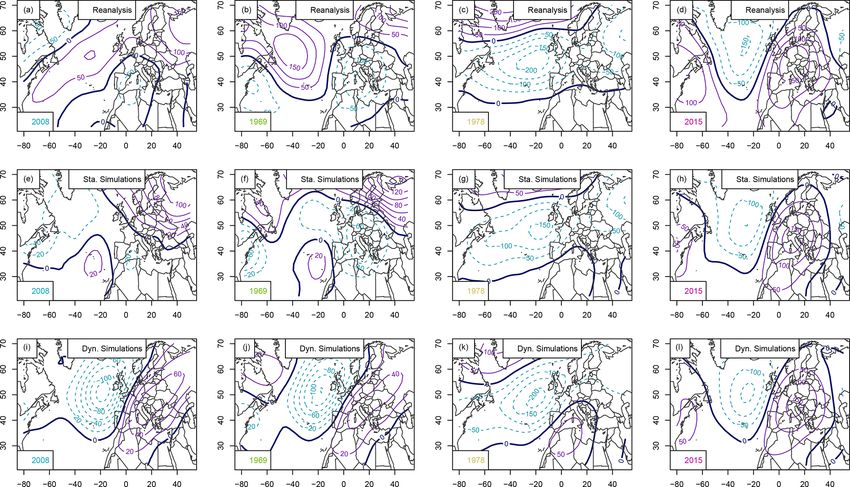
P. Pfleiderer et al.: Simulating weather extremes with stochastic weather generators                                            105

tation. The rationale of ensemble simulations is to determine        algorithm to simulate extreme heatwaves with an intermedi-
uncertainties in the range of values that can be obtained.           ate complexity climate model.
   Section 2 details the data that is used in this paper and            The procedure of importance sampling algorithms, say to
explains the methodology of importance sampling with ana-            simulate extreme heatwaves with a climate model, is to start
logue simulators. Section 3 describes the experimental re-           from an ensemble of S initial conditions and compute trajec-
sults of the simulations of temperature and precipitation. Sec-      tories of the climate model from those initial conditions.
tion 4 provides a discussion of the results.                            An optimization “observable” is defined for the system. In
                                                                     this case, it can be the spatially averaged temperature or pre-
                                                                     cipitation over France. The trajectories for which the observ-
2     Methods                                                        able (e.g. daily average temperature) is lowest during the first
                                                                     steps of simulation are deleted and replaced by small pertur-
2.1    Data                                                          bations of remaining ones. In this way, each time increment
                                                                     of the simulations keeps the trajectories with the highest val-
We use temperature and precipitation observations from the
                                                                     ues of the observable. At the end of a simulation, one obtains
E-OBS database (Haylock et al., 2008). The data are avail-
                                                                     S trajectories for which the observable (here average temper-
able on a 0.1×0.1◦ grid from 1950 to 2018. As an estimate of
                                                                     ature over France) has been maximized. Since those trajec-
temperature and precipitation in northern France we average
                                                                     tories are solutions of the equations of a climate model, they
these two fields over a rectangle spanning 45.5–51.5◦ N and
                                                                     are necessarily physically consistent (given that the perturba-
1.5◦ W–8.0◦ E (see Fig. 1). This region also includes parts of
                                                                     tions are small).
the UK, Germany, Belgium, and Switzerland and therefore
                                                                        Ragone et al. (2017) argue that the probability of the simu-
does not exactly match the studied area of (Ben-Ari et al.,
                                                                     lated trajectories is controlled by a parameter that weighs the
2018). The seasonal meteorological conditions we study here
                                                                     importance to the highest observable values: if one trajectory
are related to large-scale events, and averaging over a larger
                                                                     is deleted at each time step, the simulation of an ensemble of
rectangle therefore seems appropriate.
                                                                     M-long trajectories has a probability of (1 − 1/S)M . Hence,
   We use the reanalysis data of the National Centers for En-
                                                                     one obtains a set of S trajectories with very low probability
vironmental Prediction (NCEP) (Kistler et al., 2001) for the
                                                                     after M time increments at the cost of the computation of S
analysis of atmospheric circulation. We consider the geopo-
                                                                     trajectories.
tential height at 500 hPa (Z500) and mean sea level pres-
                                                                        For comparison purposes, if one wants to obtain S trajec-
sure (SLP) over the North Atlantic region for computation of
                                                                     tories that have a low probability (p) observable, then the
circulation analogues and a posteriori diagnostics. We used
                                                                     number of necessary “unconstrained” simulations is of the
the daily averages between 1 January 1950 and 31 Decem-
                                                                     order of M/p, so that most of those simulations are left out.
ber 2018. The horizontal resolution is 2.5◦ in longitude and
                                                                     Systems like weather@home (Massey et al., 2015b) that gen-
latitude. The rationale of using this reanalysis is that it covers
                                                                     erate tens of thousands of climate simulations are just suffi-
70 years and is regularly updated.
                                                                     cient to obtain S = 100 centennial heatwaves, and the num-
   One of the caveats of this reanalysis dataset is the lack
                                                                     ber of “wasted” simulations is very high. Therefore, impor-
of homogeneity of assimilated data, especially before the
                                                                     tance sampling algorithms are very efficient ways to circum-
satellite era. This can lead to breaks in pressure-related vari-
                                                                     vent this difficulty. The major caveat of this approach is that
ables, although such breaks are mostly detected in the South-
                                                                     one needs to know the equations that drive the system and
ern Hemisphere and the Arctic region (Sturaro, 2003) and
                                                                     be able to simulate them. We use an alternative method that
marginally impact the eastern North Atlantic region.
                                                                     does not require such knowledge of the system.
   Z500 patterns are well correlated with western European
                                                                        We use two SWG-based circulation analogues (Yiou and
temperature and precipitation because those quantities and
                                                                     Jézéquel, 2020) to simulate events of either warm temper-
their extremes are related to the atmospheric circulation
                                                                     ature in December or high precipitation in spring. These
(Yiou and Nogaj, 2004; Cassou et al., 2005). Since Z500
                                                                     SWGs resample daily weather observations in a plausible
values depend on temperature, we detrend the Z500 daily
                                                                     manner to simulate new weather events (Yiou, 2014).
field by removing a seasonal average linear trend from each
                                                                        Circulation analogues are computed on SLP (or detrended
grid point. This preprocessing is performed to ensure that the
                                                                     Z500) from NCEP between 1950 and 2018. For each day in
analogue selection is not influenced by atmospheric trends.
                                                                     1950–2018, K = 20 best analogues are determined by mini-
                                                                     mizing a spatial Euclidean distance between SLP (or Z500)
2.2    Stochastic weather generators and importance                  maps.
       sampling                                                         As explained by Yiou and Jézéquel (2020), the SWG ran-
                                                                     domly samples analogues by weighting the analogue days
The idea behind importance sampling is to simulate trajecto-         with a criterion that favours high temperatures or high pre-
ries of a physical system that optimize a criterion in a com-        cipitation. Hence, the importance sampling is summarized
putationally efficient way. Ragone et al. (2017) used such an        by the procedure of giving more weight to analogues that

https://doi.org/10.5194/esd-12-103-2021                                                 Earth Syst. Dynam., 12, 103–120, 2021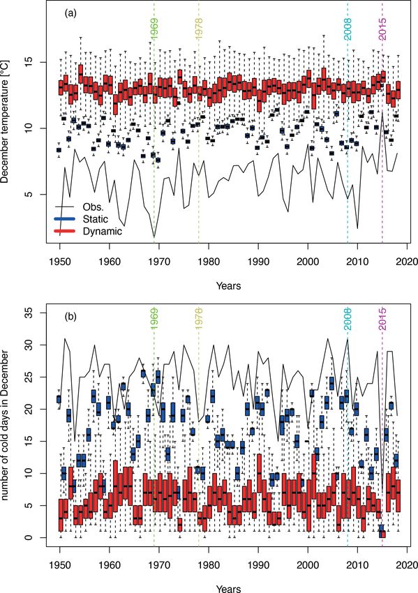
106                                        P. Pfleiderer et al.: Simulating weather extremes with stochastic weather generators

Figure 1. Regions used to identify circulation analogues for December temperatures (blue) and spring precipitation (red). The black rectangle
indicates the region over which temperatures and precipitation are averaged in northern France.

yield temperature (or precipitation) properties. There are two              An importance sampling is applied while selecting an ana-
types of importance sampling for the analogues, which are                logue at each time step by weighing probabilities with the
illustrated in Fig. 2.                                                   variable to be optimized (temperature or precipitation). The
   The two main types of analogue SWGs are described by                  K = 20 best analogues and the day of interest are sorted
Yiou (2014) and Yiou and Jézéquel (2020) are as follows:                 by daily mean temperature or precipitation. The probability
                                                                         weights are determined by Yiou and Jézéquel (2020). If R(k)
  1. A “static” weather generator replaces each day with one
                                                                         is the rank (in terms of temperature or precipitation) of day
     of its K circulation analogues or itself. With this type of
                                                                         k in decreasing order and ωk the probability of day k to be
     SWG, simulated trajectories are perturbations (by ana-
                                                                         selected, we set
     logues) of an observed trajectory.
                                                                         ωk = Ae−αR(k) ,                                                 (2)
  2. A so-called “dynamic” weather generator has a similar
     random selection rule, but the “next” day to be simu-               where A is a normalizing constant so that the sum of weights
     lated follows the selected analogue, rather than the ob-            over k is 1. The α parameter controls the strength of this im-
     served actual calendar day. A probability weight ωcal               portance sampling for temperature or precipitation.
     that is inversely proportional to the distance to the cal-             The useful property of this formulation of weights is that
     endar day is introduced:                                            the values of ωk do not depend on time t because the rank
                                                                         values R(k) are integers between 1 and K + 1. The weight
      ωcal = Acal e−αcal Rcal (k) ,                             (1)      values do not depend on the unit of the variable either, and
                                                                         thus this procedure is the same for temperature or precipita-
      where Acal is a normalizing constant, αcal ≥ 0 is a
                                                                         tion. If α = 0, this is equivalent to a stochastic weather gen-
      weight, and Rcal (k) is the number of days that separate
                                                                         erator described by Yiou (2014).
      the date of kth analogue from the calendar day of time t.
                                                                            Combining the weights of the calendar day and the inten-
      This rule is important to prevent time from going “back-
                                                                         sity of the climate variable, the probability of day k to be
      ward”. This type of SWG generates new trajectories by
                                                                         selected becomes
      resampling already observed ones. They are not just per-
      turbations of observed trajectories.                               ωk0 = Ae−αR(k) e−αcal Rcal (k) .                                (3)
Those random selections of analogues are sequentially re-                  The generators thus give more weight to the warmest or
peated until a lead time T .                                             wettest days when computing trajectories of December tem-

Earth Syst. Dynam., 12, 103–120, 2021                                                         https://doi.org/10.5194/esd-12-103-2021
P. Pfleiderer et al.: Simulating weather extremes with stochastic weather generators 107
Figure 2. Illustration of the analogue-based importance sampling. (a) The static SWG replaces each day in the observed trajectory (black
dots) with one of its analogues (red dots). (b) The dynamic SWG replaces the first day in the observations (black dot) with one of its
analogues, reads the following day of this analogue, and repeats the procedure until creating a new trajectory (red dots).
perature or spring precipitation. We thereby simulate extreme 30–70◦ N and 50◦ W–30◦ E, as shown in Fig. 1. This re-
events, e.g. warm Decembers and wet springs (May to July). gion includes large parts of the North Atlantic where
rain-bringing storms usually come from.
2.3 Experimental set-up
– Number of days before selecting a new analogue. For
The parameters of the SWG depend on the variables and the the simulation of long-lasting precipitation events the
seasons to be simulated. We determine those parameters ex- consistency of day-to-day variability is important to en-
perimentally and detail them hereafter. Table 1 lists all pa- sure a plausible water vapour transport. We therefore
rameters used for the simulation of December temperature adapt the stochastic weather generator (both static and
and spring precipitation. These parameters were set after per- dynamic). Instead of choosing a new analogue every
forming a number of sensitivity tests that are going to be dis- day, we stay on an observed trajectory for a number
cussed in Sect. 3. Table 2 lists all values tested for α and of days (ndays ) before choosing a new analogue (see
αcal . Most figures related to these tests can be found in the Fig. 3). For the analogue selection we weight the ana-
Appendix. logues based on the accumulated precipitation of the
The procedure we follow is as follows. analogue and the following ndays days, giving more
– Start and end day of simulations. For each year from weight to analogues that bring more precipitation in the
1950 to 2018, 1000 simulations are started indepen- following ndays days.
dently for temperature in December and precipitation
– Selection of circulation analogues by the generators.
in spring. The temperature simulations start on 1 De-
The α-parameter controls the strength of the importance
cember and end on 31 December. Precipitation simula-
sampling on either temperature or precipitation, while
tions start on 1 April and end on 31 July. This results in
αcal controls the influence of the calendar date when
68 000 independent simulations of December tempera-
selecting an analogue. For temperature simulations, we
tures and spring precipitation.
use α = 0.75 and αcal = 6. Note that we thus strongly
– Identification of circulation analogues. Weather ana- condition the calendar day to restrict the SWGs to win-
logues are identified by evaluating the similarity of ter and late autumn days. For precipitation, we set both
weather patterns of an atmospheric variable in a cho- α and αcal to 0.5.
sen region. For December temperature, analogues are
based on detrended geopotential height at 500 hPa
(Z500) over a region covering most of Europe (70– 3 Results
23◦ N, 10◦ W–40◦ E) (see Fig. 1). Jézéquel et al. (2018)
showed that Z500 is better suited to simulate tempera- A lack of cold days in December 2015 and an exception-
ture anomalies than SLP and that rather small domains ally wet spring caused the 2016 crop loss in northern France.
lead to better reconstitutions. This result is supported by Although the interplay between these two meteorological
sensitivity tests we performed on the choice of variable events is crucial for the resulting crop loss, the two events
for the computation of the circulation analogues used (warm December and wet spring) seem to have happened in-
to simulate December temperature. For spring precipi- dependently from each other: the correlation between tem-
tation, we use analogues of SLP over a zone covering perature in December and precipitation 4 months later is not
https://doi.org/10.5194/esd-12-103-2021 Earth Syst. Dynam., 12, 103–120, 2021108 P. Pfleiderer et al.: Simulating weather extremes with stochastic weather generators
Table 1. Parameters used for the static and dynamic SWG to simulate warm Decembers (second column) and wet April–July periods (last
column).
Parameter Choice for warm Decembers Choice for wet April–July periods
Start day 01/12 01/04
End day 31/12 31/07
Variable for analogues Z500 SLP
Region for analogues 70–23◦ N, 10◦ W–40◦ E 30–70◦ N and −50◦ W–30◦ E 30–70◦ N
Weighting of temp. or precipitation (α) 0.75 0.5
Weighting of calendar day (αcal ) 6 0.5
Number of days before
selecting a new analogue (ndays ) 1 5
Table 2. Performed sensitivity tests for the parameters used to simulate warm Decembers (first three rows) and wet April–July periods (last
three rows). The second column lists the parameters of which the sensitivity is assessed. The third column indicates at which levels all other
parameters are fixed for the test. The fourth column lists all tested values and the last column indicates the figure where the results of the test
are shown.
Experiment Tested parameter Fixed parameters Tested values Figure
December variable for analogues α = 0.5, αcal = 6, ndays = 1 Z500, SLP Fig. A1
December αcal α = 0.5, ndays = 1 0, 0.2, 0.5, 1, 2, 4, 6, 8, 10 Fig. A2
December α αcal = 6, ndays = 1 0, 0.1, 0.2, 0.5, 0.75, 1 Fig. A3
April–July ndays α = 0.5, αcal = 0.5 1, 2, 3, 4, 5, 7, 9 Fig. A4
April–July α αcal = 0.5, ndays = 5 0, 0.1, 0.3, 0.5, 0.7, 0.9, 1 Fig. A5
April–July αcal α = 0.5, ndays = 5 0, 0.2, 0.5, 1, 2, 5, 10 Fig. A6
significantly different from zero and we cannot reject the hy- the starting day and is therefore less bound to each year’s
pothesis that both variables are not correlated (p value of circulation.
the Pearson correlation > 0.6). In addition, from an energy In years with higher December temperatures, the num-
point of view, the characteristic timescale of the atmosphere ber of cold days with maximal temperatures between 0 and
does not exceed 35 d (Peixoto and Oort, 1992, Sect. 14.6.2). 10 ◦ C is reduced (see Fig. 4b). Over the period 1950–2018 no
This implies that it is unlikely to find links between climate trend in the number of cold days is observed and the number
variables in December and the following May. We therefore of cold days fluctuates around 25 d. As the SWG simulates
consider that it is reasonable to simulate warm Decembers warmer Decembers the number of cold days is on average
and wet springs independently. 8 d lower in the static SWG and 16 d lower in the dynamic
SWG. Nearly half of the simulations of the dynamic SWG
3.1 December temperature simulations thus have fewer cold days than what was observed in De-
cember 2015.
The winter preceding the 2016 crop loss was abnormally December 2015 was unprecedented in terms of missing
warm, with only a few cold days. Here, cold days are de- cold days, and we simulate a number of warm Decembers
fined as days with daily maximal temperatures between 0 and with even fewer cold days. To estimate the probability of
10 ◦ C. This December was the hottest in the observational such an extreme December, we fit a beta-binomial distribu-
record and also the December with the fewest cold days. tion (Jézéquel et al., 2018) to the observations and find that
Figure 4a shows the observed averages of daily maximal 2015 was a 1-in-4000-year event and that 25 % of our dy-
temperatures and the results from static and dynamic SWG namic SWG simulations are 1-in-1000-year events or even
simulations. The observed December temperatures fluctu- rarer (see Fig. A3).
ate around 6 ◦ C, with a small warming trend of 0.2 ◦ C per As shown in Fig. 5, December 2015 was characterized by
decade over the whole time series (p value = 0.03). Simu- a persistent anticyclonic circulation with its centre over the
lations from the static SWG are consistently around 3.5 ◦ C Alps. The circulation in the coldest December (1969) was
warmer and follow the year-to-year variability of the obser- the opposite of 2015, with negative Z500 anomalies over Eu-
vations. With an average of 12 ◦ C, the dynamic SWG sim- rope and positive anomalies over the Atlantic. In 2008, the
ulations are significantly warmer than the static SWG simu- December with most cold days in the observations, the data
lations, and inter-annual variability is strongly reduced. This resemble 1969 but have less pronounced anomalies.
is to be expected as the dynamic SWG evolves freely from
Earth Syst. Dynam., 12, 103–120, 2021 https://doi.org/10.5194/esd-12-103-2021P. Pfleiderer et al.: Simulating weather extremes with stochastic weather generators 109
Figure 3. Adapted dynamic weather generators. (a) The adapted static SWG selects a new analogue every nth day (4 d in this illustration)
and follows the observed trajectory (dotted black line) of that day for 3 d. The resulting simulation combines observed 4 d chunks into an
artificial trajectory (red line). (b) The adapted dynamic SWG replaces the first day of the observations with one of its analogues and follows
the observed trajectory of that analogue for 3 d. Following this, a new analogue of the following day in the observed trajectory is chosen.
For all example years, the circulation in the static SWG simulations even reach daily mean precipitation of 6 mm for
simulations exhibits the same features as the observed cir- April–July, which is 3 times as high as the observed precipi-
culation. The dynamic SWG always simulates high-pressure tation in 1983.
anomalies over France irrespective of the starting conditions. April–July periods simulated by the dynamic SWG are
These anomalies are, however, more pronounced in 2015 even wetter than the simulations of the static SWG, with an
where the starting circulation favours the anticyclonic pat- average seasonal precipitation of 590 mm. As expected, the
tern over France. inter-annual variations are smaller in the dynamic SWG sim-
The simulations of warm Decembers are most sensitive to ulations than in the static SWG simulations because the dy-
the weighting of the calendar date. If this parameter is chosen namic SWG evolves freely, with the starting conditions their
too loosely, simulations would include days from other sea- only link to the observed circulation.
sons, which are generally warmer. As shown in Fig. A2, for We estimate the return periods of our simulated events by
αcal ≥ 6 over 70 % of all days in the simulations are sampled fitting a normal distribution to the observed April–July pre-
from the November–February period. Increasing the weight- cipitation events. As we average over a quite large region and
ing of the calendar day further does not show a significant over 4 months, a normal distribution represents the observa-
effect. tions well (even though the analysed variable is precipita-
The simulations are also sensitive to the weighting of daily tion). We find that the 2016 April–July period was a 1-in-17-
maximal temperatures α (Fig. A3). For α ≥ 0.75 we simu- year event, while the majority of our SWGs simulations are
late a large number of Decembers that are more extreme than 1-in-10 000-year events.
2015. In April–July 2016, the atmospheric circulation was char-
Finally, the choice of geopotential height or mean sea level acterized by a moderate low-pressure anomaly north of
pressure to classify circulation analogues does not influence France and north of the Azores (Fig. 7a). The North Atlantic
the simulations (see Fig. A1). Oscillation (NAO) index switched from slightly positive to
negative in May and remained negative until the end of June
(NOAA, 2020).
3.2 Spring precipitation
We next analyse the large-scale atmospheric circulation
An extremely wet period from April to July 2016 followed patterns that characterize our SWG simulations by compar-
the warm December in 2015, with an average precipitation ing them to a few examples of observed events. Figure 7a–
of 2.7 mm per day and 332 mm for the whole period. This is d shows the mean sea level composites of 2016, the driest
more than the long-term 75th percentile, but it is topped by (1976), the median (1986), and the wettest (1983) April–July
some years including 1983, 1987, and 2012. periods. The main feature in the median event (Fig. 7c) is
Figure 6 shows the daily mean precipitation for April–July a low pressure anomaly north-westward of the British Isles.
periods over 1950–2018. Accumulated April–July precipi- The wettest event (Fig. 7d) is characterized by a strong dipole
tation fluctuates around 256 mm with a strong year-to-year over the North Atlantic with low pressure in the east and high
variability. Over the observed period no trend is detected. pressure in the west. In the driest event (Fig. 7b) this dipole
Simulations from the static weather generator (blue box- is reversed and slightly shifted to the east.
plots in Fig. 6) also show a strong inter-annual variability but For all four events, the static SWG tends to create events
have significantly larger amounts of precipitation. The aver- with stronger low pressure anomalies over northern France
age seasonal precipitation for all simulations and all years (Fig. 7e–h). Similarly, the simulations from the dynamic
is around 487 mm–190 % of the observed average. Single SWG all show a strong low-pressure anomaly over north-
https://doi.org/10.5194/esd-12-103-2021 Earth Syst. Dynam., 12, 103–120, 2021110 P. Pfleiderer et al.: Simulating weather extremes with stochastic weather generators
in 2016. In contrast to the persistent anticyclonic anomaly
that led to a continuously warm December in 2015, the wet
April–July period was favoured by a number of storms pass-
ing over northern France.
Our simulations of April–July periods combine 5 d chunks
of observed weather into one coherent time series. By using
5 d chunks instead of combining single-day observations, we
constrain our simulations to observed day-to-day variations
that appear to be crucially important for precipitation events.
This ensures that in our simulations storms predominantly
travel eastwards and that the moisture transport in the simu-
lations is reasonable – at least during the 5 d in question (see
the animated .gif files in the Supplement).
Sensitivity tests indeed show that simulations where a new
analogue is chosen every day result in significantly higher
precipitation, with 7 mm per day for the dynamic SWG sim-
ulations (see Fig. A4). The amount of precipitation steadily
decreases with the length of the observed chunks that are
assembled by the SWGs (ndays ). This is to be expected, as
with longer assembled chunks and fewer analogue choices
the simulated weather events resemble the observations more
and more. There is an especially strong decrease in simulated
precipitation from 1 to 3 d, which suggests that when ana-
logues are chosen more frequently than every third day po-
tentially unreasonable weather events are created. Note that
taking 5 d windows is a heuristic choice and that window
sizes between 4 and 7 d give similar results.
The simulations are by definition sensitive to the weight-
ing of the amount of precipitation α. As shown in Fig. A5,
with a relatively small weight of 0.1 most dynamic simu-
Figure 4. (a) Daily maximal temperature in December from 1950
lations already bring more precipitation than what was ob-
to 2018. The black line shows E-OBS observations. The boxplots
represent the ensemble variability of the simulations of the static
served in 2016. This could be due to the length of the simula-
(blue) and the dynamic (red) SWG for each year. The boxes of tions: it is rather unlikely that extreme weather endures over
the boxplots indicate the median (q50) and lower (q25) and up- 4 months. However, with a weak weighting of wet weather
per (q75) quartiles. The upper whiskers indicate min[max(T ), 1.5× simulations can already result in a long-lasting consistent wet
(q75 − q25)]. The lower whisker has a symmetrical formulation. periods. This increase in precipitation saturates after α ≈ 0.5,
The points are the simulated values that are above or below the de- and increasing α further has no effect on the final results.
fined whiskers. Panel (b) is the same as (a) but for the number of As for the other free parameters of the SWG, this sensitiv-
cold days. The coloured vertical lines indicate the coldest Decem- ity test does not directly justify the choice of the parameter
ber (green), a median December (yellow), a December with 31 cold α. It instead gives guidance on the values that would be ap-
days (cyan) and the warmest December (purple). propriate choices for our application. In the end the parame-
ter is heuristically chosen considering the trade-off between
creating high-precipitation events and keeping as much ran-
ern France (Fig. 7i–l). For the dynamic SWG simulations, domness as possible in our simulations.
even in 1976, which was the driest April–July period, a low- As shown in Fig. A6, the weighting of the calendar day has
pressure anomaly is simulated for northern France where a limited influence on the amount of precipitation in northern
high-pressure system had been observed. In the static SWG, France simulated by our SWGs.
the high-pressure anomaly is relocated to the west, also lead- For precipitation in northern France the weighting of the
ing to a low-pressure anomaly over northern France. calendar day is less relevant as there is no pronounced sea-
Besides a general tendency towards low-pressure anoma- sonal cycle in precipitation (see Fig. A6).
lies over northern France, the 2016 April–July period was Finally, one feature in the simulations of April–July de-
characterized by an increased daily pressure variability west serves some more attention: for both static and dynamic
of France (compare Figs. B1a and c). This indicates an en- SWG simulations precipitation is exceptionally high in 1994
hanced storm track activity downstream of our region of in- and 1998. Although observed precipitation in these years was
terest and could explain the increased precipitation observed relatively high, this cannot explain the amount of precipi-
Earth Syst. Dynam., 12, 103–120, 2021 https://doi.org/10.5194/esd-12-103-2021P. Pfleiderer et al.: Simulating weather extremes with stochastic weather generators 111
Figure 5. Geopotential height anomaly at 500 hPa (Z500) composites for a year with 31 cold days (2008), the coldest December (1969), the
median (1978), and the warmest December (2015): (a–c) mean Z500 from NCEP reanalyses, (d–f) static SWG simulations, (g–i) dynamic
SWG simulations. Isolines are shown with 100 m increments. Positive Z500 anomalies are shown with continuous purple isolines, negative
anomalies are shown with dashed cyan lines, and the 500 hPa isoline is shown with a continuous thick black line.
tation in the simulations. One explanation for these outlier The warm December in 2015 resulted in very few cold
years could be a loop in the simulations leading to an exces- days with temperatures between 0 and 10 ◦ C. Our simula-
sive repetition of the same (wet) sequence of days. As shown tions show that substantially warmer Decembers would be
in Fig. A7, in 1998 one date is indeed repeated 10 times in possible. However, in terms of cold days, which is a more
both the static and dynamic weather generator. In most other relevant indicator for wheat phenology in that season (Ben-
years, repetitions of single dates are rare. As our results do Ari et al., 2018), December 2015 was already extreme, and
not rely on simulations of single years, this feature does not only a few simulations show lower numbers of cold days.
affect the overall findings of the study. For April–July precipitation, we find that much wetter pe-
These simulations show that there are many possible riods than what was observed in 2016 would be plausible.
April–July periods that would be significantly wetter than The simulated events bring more than twice as much precip-
what was observed in 2016 and also wetter than the observed itation than in 2016.
record precipitation (1983). If crop yields responds to the number of cold days in win-
ter and to the precipitation rate in spring, as shown in Ben-Ari
4 Discussion et al. (2018), then we have shown here that in the current cli-
mate an even worse crop loss event would be possible. The
In 2016 northern France suffered an unprecedented crop loss April–July period in particular could be significantly wetter
that can be related to an abnormally warm December in than what was observed in 2016.
2015 and a following wet April–July period in 2016 (Ben- We used stochastic weather generators to simulate extreme
Ari et al., 2016). Here we investigated how extreme these but plausible weather events. While the method is estab-
meteorological precursors of the crop loss could be in the lished for summer heat waves (Yiou and Jézéquel, 2020), the
current climate. Using stochastic weather generators (SWG) weather events we studied here brought new challenges: al-
we simulate warm Decembers and wet April–July periods though the circulation pattern of the warm December 2015
independently. was similar to a summer heat wave with an anticyclonic pat-
tern over France, special care was required to assure that our
https://doi.org/10.5194/esd-12-103-2021 Earth Syst. Dynam., 12, 103–120, 2021112 P. Pfleiderer et al.: Simulating weather extremes with stochastic weather generators
To further evaluate the plausibility of our simulations one
could also compare them to extreme events simulated by
large ensemble climate modelling experiments. In a study
using a near-term climate prediction model, Thompson et al.
(2017) found that for England there is a considerable chance
of unprecedented winter rainfall. Replicating a similar study
for northern France spring precipitation would not only pro-
vide an alternative estimate of extreme spring precipitation
but would also allow us to further evaluate the circulation
features of our weather simulations.
Finally, our simulated extremes could be used as input for
the regression-based yield model of Ben-Ari et al. (2018).
These results should, however, be interpreted cautiously as
our simulated weather extremes lie outside of the observed
range and therefore also the range within which the yield
Figure 6. Daily precipitation averages for April–July from 1950 to
model was trained. They could also be used in process-based
2018. The black line shows E-OBS observations. The boxplots rep-
crop models as a worst-case meteorological scenario.
resent the ensemble variability of the simulations of the static (blue)
and the dynamic (red) SWG for each year. The boxes of boxplots
indicate the median (q50), lower (q25), and upper (q75) quartiles. 5 Conclusions
The upper whiskers indicate min[max(T ), 1.5 × (q75 − q25)]. The
lower whisker has a symmetrical formulation. The points are the This paper is a proof of concept for the importance sampling
simulated values that are above or below the defined whiskers. The for a simulation of a compound event (warm autumn-winter
coloured vertical lines indicate the driest April–July period (1976), and wet spring) that would have an impact on crop yield. It
the wettest period (1983), a median period (1986), and 2016. relies on a data-resampling approach to maximize tempera-
ture and precipitation over extended periods of time.
The simulations are based on the a priori knowledge (from
simulated events are actually realizations of winter weather. expertise on crop failures in northern France) that warm au-
Here we assured for this by strongly weighting the calendar tumns and winters followed by wet springs have detrimental
date when selecting analogues. effects on crops.
The wet April–July 2016 period was characterized by a The first application of SWGs to warm winter periods and
series of passing storms that brought considerable amounts wet springs is an important advance in this research field. It
of precipitation. The main feature of this wet spring season also shows that with only a few adaptations SWGs can be ap-
was therefore not persistence and simulating plausible day- plied to new weather phenomena, highlighting the merits of
to-day variations with SWGs was a major challenge. SWGs the method. Moreover, the SWG parameters can be adapted
that select a new analogue every day tend to simulate persis- to other types of crops (with other phenological parameters
tent rainfall events over spring, with little day-to-day varia- and key dates).
tion. This approach is rather flexible and could be adapted to
As a first attempt to simulate plausible long lasting wet simulate compound extremes using climate model outputs
periods, we propose to reassemble 5 d windows of observed based on different scenarios of climate change. This could
weather instead of single days. This ensures that low- and lead to the first evaluation of the impact of climate change
high-pressure systems predominantly travel eastward at a on worst-case scenarios of crop yields. This type of analy-
speed that is tightly linked to observations. An alternative ap- sis has some limitations related to the uncertainty of models
proach could be to switch trajectories on dry days instead of and scenarios, and it fails to take into account non-climatic
switching after a fixed number of days. This would addition- drivers of crop yields such as pests, supply chains, or eco-
ally avoid changing trajectories during precipitation events. nomical concerns. However, we believe it could be useful to
Evaluating the plausibility of our simulations remains a estimate what could be plausible in terms of purely meteoro-
challenge: although sensitivity tests and an analysis of the logical events in a changing climate.
simulated circulation patterns reveal the robust and clearly
interpretable behaviour of SWGs, further tests would be re-
quired to assess whether all simulated events could really
happen in our climate. It could, for instance, be interesting
to analyse the simulated wet April–July periods with respect
to more climate variables (e.g. relative humidity) to evaluate
whether the water transport is physically plausible through-
out the simulated period.
Earth Syst. Dynam., 12, 103–120, 2021 https://doi.org/10.5194/esd-12-103-2021P. Pfleiderer et al.: Simulating weather extremes with stochastic weather generators 113 Figure 7. SLP anomaly composites (Pa) for April–July 2016, the driest period, the median (1986), and the wettest period (1983): (a–d) mean SLP from NCEP reanalyses, (e–h) static SWG simulations, (i–l) dynamic SWG simulations. Isolines are shown with 100 Pa increments. Positive SLP anomalies are shown with continuous purple isolines, negative anomalies are shown with dashed cyan lines, and the mean SLP isoline is shown with a continuous thick black line. https://doi.org/10.5194/esd-12-103-2021 Earth Syst. Dynam., 12, 103–120, 2021
114                                        P. Pfleiderer et al.: Simulating weather extremes with stochastic weather generators

Appendix A: Sensitivity tests

A1    December temperature

                                                                       Figure A2. Percentage of days sampled between November and
                                                                       February by the dynamic generator when running 100 simulations
                                                                       of December temperatures as a function of the parameter αcal . The
                                                                       dotted red line is for αcal = 6 (which is the value used in the analy-
Figure A1. Distribution of the daily maximum temperature in De-        sis).
cember averaged in observations (white) and in simulations com-
puted by the static (blue) and dynamic (red) generators using circu-
lation analogues computed using the SLP or Z500. The horizontal
dotted line corresponds to the daily maximum temperature observed
in December 2015. The boxes of boxplots indicate the median
(q50), lower (q25), and upper (q75) quantiles. The upper whiskers
indicate min[max(T ),1.5 × (q75−q25)]. The lower whisker has a
symmetrical formulation. The points are the simulated values that
are above or below the defined whiskers.

Earth Syst. Dynam., 12, 103–120, 2021                                                      https://doi.org/10.5194/esd-12-103-2021
P. Pfleiderer et al.: Simulating weather extremes with stochastic weather generators 115
A2 Spring precipitation
Figure A3. Distribution of the number of December days with max-
imal temperatures between 0 and 10 ◦ C in observations (white) and
in simulations computed by the static (blue) and dynamic (red) gen-
erators as a function of α. The axis on the right indicates the prob-
ability of occurrence, assuming a beta-binomial distribution of the Figure A4. Distribution of April–July daily precipitation in obser-
number of winter days with parameters estimated from white box- vations (white) and in simulations computed by the static (blue) and
plot. The horizontal dotted line corresponds to the observed num- dynamic (red) generators as a function of the number of days before
ber of days in December 2015. The boxes of boxplots indicate selecting a new analogue ndays . The axis on the right indicates the
the median (q50), lower (q25), and upper (q75) quartiles. The up- probability of occurrence, assuming a normal distribution of daily
per whiskers indicate min[max(T ), 1.5 × (q75 − q25)]. The lower precipitation with parameters estimated from white boxplot. The
whisker has a symmetrical formulation. The points are the simu- horizontal dotted line corresponds to the observed daily precipita-
lated values that are above or below the defined whiskers. tion in April–July 2016. The boxes of boxplots indicate the median
(q50), lower (q25), and upper (q75) quartiles. The upper whiskers
indicate min[max(T ), 1.5 × (q75 − q25)]. The lower whisker has a
symmetrical formulation. The points are the simulated values that
are above or below the defined whiskers.
https://doi.org/10.5194/esd-12-103-2021 Earth Syst. Dynam., 12, 103–120, 2021116 P. Pfleiderer et al.: Simulating weather extremes with stochastic weather generators Figure A5. Distribution of April–July daily precipitation in obser- Figure A6. Distribution of April–July daily precipitation in obser- vations (white) and in simulations computed by the static (blue) and vations (white) and in simulations computed by the static (blue) and dynamic (red) generators as a function of α. The axis on the right dynamic (red) generators as a function of αcal . The axis on the right indicates the probability of occurrence, assuming a normal distri- indicates the probability of occurrence, assuming a normal distri- bution of daily precipitation with parameters estimated from white bution of daily precipitation with parameters estimated from the boxplot. The horizontal dotted line corresponds to the observed white boxplot. The horizontal dotted line corresponds to the ob- daily precipitation in April–July 2016. The boxes of boxplots in- served daily precipitation in April–July 2016. The boxes of boxplots dicate the median (q50), lower (q25), and upper (q75) quartiles. indicate the median (q50), lower (q25), and upper (q75) quartiles. The upper whiskers indicate min[max(T ), 1.5 × (q75 − q25)]. The The upper whiskers indicate min[max(T ), 1.5 × (q75 − q25)]. The lower whisker has a symmetrical formulation. The points are the lower whisker has a symmetrical formulation. The points are the simulated values that are above or below the defined whiskers. simulated values that are above or below the defined whiskers. Earth Syst. Dynam., 12, 103–120, 2021 https://doi.org/10.5194/esd-12-103-2021
P. Pfleiderer et al.: Simulating weather extremes with stochastic weather generators                                                   117

Figure A7. Maximal number of times a single date is repeated for each simulated year. The boxplots indicate the range of this maximal
repetition number for the 1000 simulations for simulations of the static (blue) and dynamic (red) stochastic weather generator. The boxes of
boxplots indicate the median (q50), lower (q25), and upper (q75) quartiles. The upper whiskers indicate min[max(T ), 1.5 × (q75 − q25)].
The lower whisker has a symmetrical formulation. The points are the simulated values that are above or below the defined whiskers.

https://doi.org/10.5194/esd-12-103-2021                                                      Earth Syst. Dynam., 12, 103–120, 2021
118                                      P. Pfleiderer et al.: Simulating weather extremes with stochastic weather generators

Appendix B: Circulation details

Figure B1. Standard deviation of daily SLP anomalies (Pa) for April–July 2016, the driest period, the median (1986), and 2018: (a–d) SLP
from NCEP reanalyses, (e–h) static SWG simulations, (i–l) dynamic SWG simulations. For the SWG simulations the average of all 1000
runs for the given year is presented.

Earth Syst. Dynam., 12, 103–120, 2021                                                     https://doi.org/10.5194/esd-12-103-2021
P. Pfleiderer et al.: Simulating weather extremes with stochastic weather generators                                                    119

Code availability. All     R scripts used for the analysis            Ben-Ari, T., Boé, J., Ciais, P., Lecerf, R., Van der Velde, M., and
and the production of figures are openly available under                 Makowski, D.: Causes and implications of the unforeseen 2016
https://doi.org/10.5281/zenodo.4327671 (Pfleiderer et al., 2020).        extreme yield loss in the breadbasket of France, Nat. Commun.,
                                                                         9, 1627, https://doi.org/10.1038/s41467-018-04087-x, 2018.
                                                                      Cassou, C., Terray, L., and Phillips, A. S.: Tropical Atlantic influ-
Supplement. The supplement related to this article is available          ence on European heat waves, J. Climate, 18, 2805–2811, 2005.
online at: https://doi.org/10.5194/esd-12-103-2021-supplement.        Cooley, D.: Extreme value analysis and the study of climate change,
                                                                         Climatic Change, 97, 77–83, 2009.
                                                                      de Bruijn, K. M., Lips, N., Gersonius, B., and Middelkoop,
Author contributions. PY and AJ conceived the study. NL, JL,             H.: The storyline approach: a new way to analyse and im-
IM, EV, and PP did the analysis and created all figures. PP wrote        prove flood event management, Nat. Hazards, 81, 99–121,
the manuscript with contributions from all authors.                      https://doi.org/10.1007/s11069-015-2074-2, 2016.
                                                                      FAO: Agricultural statistics database, Rome: World Agricultural,
                                                                         Information Center, available at: http://faostat.fao.org/site/567/
                                                                         DesktopDefault.aspx (last access: 22 May 2020), 2013.
Competing interests. The authors declare that they have no con-
                                                                      Haylock, M. R., Hofstra, N., Tank, A. M. G. K., Klok,
flict of interest.
                                                                         E. J., Jones, P. D., and New, M.: A European daily high-
                                                                         resolution gridded data set of surface temperature and precipi-
                                                                         tation for 1950–2006, J. Geophys. Res.-Atmos., 113, D20119,
Special issue statement. This article is part of the special issue       https://doi.org/10.1029/2008JD010,201, 2008.
“Understanding compound weather and climate events and related        Hazeleger, W., Van Den Hurk, B. J., Min, E., Van Oldenborgh, G. J.,
impacts (BG/ESD/HESS/NHESS inter-journal SI)”. It is not asso-           Petersen, A. C., Stainforth, D. A., Vasileiadou, E., and Smith,
ciated with a conference.                                                L. A.: Tales of future weather, Nat. Clim. Change, 5, 107–113,
                                                                         https://doi.org/10.1038/nclimate2450, 2015.
                                                                      Jaworski, P., Durante, F., Hardle, W. K., and Rychlik, T.: Copula
Acknowledgements. We acknowledge the E-OBS dataset from                  theory and its applications, vol. 198, Springer, Berlin, Heidel-
the EU-FP6 project UERRA (http://www.uerra.eu, last access:              berg, 2010.
20 September 2019) and the Copernicus Climate Change Service          Jézéquel, A., Cattiaux, J., Naveau, P., Radanovics, S., Ribes, A.,
and the data providers of the ECAD project (https://www.ecad.eu,         Vautard, R., Vrac, M., and Yiou, P.: Trends of atmospheric cir-
last access: 20 September 2019). We also acknowledge the NCEP            culation during singular hot days in Europe, Environ. Res. Lett.,
Reanalysis data provided by the NOAA/OAR/ESRL.                           13, 054007, https://doi.org/10.1088/1748-9326/aab5da, 2018.
                                                                      Kistler, R., Kalnay, E., Collins, W., Saha, S., White, G., Woollen, J.,
                                                                         Chelliah, M., Ebisuzaki, W., Kanamitsu, M., Kousky, V., van den
Financial support. This research has been supported by the               Dool, H., Jenne, R., and Fiorino, M.: The NCEP-NCAR 50-
DAMOCLES COST (grant no. CA17109). Peter Pfleiderer was                  year reanalysis: Monthly means CD-ROM and documentation,
supported by the German Federal Ministry of Education and                B. Am. Meteor. Soc., 82, 247–267, 2001.
Research (grant no. 01LN1711A). Edoardo Vignotto was supported        MacDonald, R. B. and Hall, F. G.: Global crop forecasting, Science,
by the Swiss National Science Foundation (Doc.CE11 Mobility              208, 670–679, 1980.
Grant no. 188229).                                                    Massey, N., Jones, R., Otto, F., Aina, T., Wilson, S., Murphy, J.,
                                                                         Hassell, D., Yamazaki, Y., and Allen, M.: weather@ home–
The publication of this article was funded by the                        development and validation of a very large ensemble modelling
Open Access Fund of the Leibniz Association.                             system for probabilistic event attribution, Q. J. Roy. Meteor. Soc.,
                                                                         141, 1528–1545, 2015a.
                                                                      Massey, N., Jones, R., Otto, F. E. L., Aina, T., Wilson,
Review statement. This paper was edited by Bart van den Hurk             S., Murphy, J. M., Hassell, D., Yamazaki, Y. H., and
and reviewed by Daithi Stone and Henrique Moreno Dumont                  Allen, M. R.: weather@home–development and validation
Goulart.                                                                 of a very large ensemble modelling system for probabilis-
                                                                         tic event attribution, Q. J. Roy. Met. Soc., 141, 1528–1545,
                                                                         https://doi.org/10.1002/qj.2455, 2015b.
                                                                      Müller, C., Elliott, J., Kelly, D., Arneth, A., Balkovic, J., Ciais,
References                                                               P., Deryng, D., Folberth, C., Hoek, S., Izaurralde, R. C., Jones,
                                                                         C. D., Khabarov, N., Lawrence, P., Liu, W., Olin, S., Pugh, T.
ARVALIS: Rendements catastrophiques du blé en 2016:                      A. M., Reddy, A., Rosenzweig, C., Ruane, A. C., Sakurai, G.,
  la pluie, seule responsable?, available at: https://www.               Schmid, E., Skalsky, R., Wang, X., de Wit, A., and Yang, H.: The
  semencesdefrance.com/actualite-semences-de-france/                     Global Gridded Crop Model Intercomparison phase 1 simulation
  rendements-catastrophiques-ble-2016-pluie-seule-responsable/           dataset, Scientific Data, 6, 1–22, 2019.
  (last access: 23 October 2020), 2016 (in French).                   NOAA: North Atlantic Oscillation, available at: https://www.cpc.
Ben-Ari, T., Adrian, J., Klein, T., Calanca, P., Van der Velde, M.,      ncep.noaa.gov/products/precip/CWlink/pna/nao.shtml, last ac-
  and Makowski, D.: Identifying indicators for extreme wheat and         cess: 10 January 2020.
  maize yield losses, Agr. Forest Meteorol., 220, 130–140, 2016.

https://doi.org/10.5194/esd-12-103-2021                                                     Earth Syst. Dynam., 12, 103–120, 2021
You can also read